DOI:10.32604/cmc.2022.021899
| Computers, Materials & Continua DOI:10.32604/cmc.2022.021899 | |
| Article |
Numerical Analysis of Laterally Loaded Long Piles in Cohesionless Soil
1Physics and Engineering Mathematics Department, Faculty of Engineering-Mattaria, Helwan University, Cairo, 11718, Egypt
2Faculty of Engineering, King Salman International University, South Sinai, Ras Sedr, Egypt
3Basic and Applied Science Department, College of Engineering and Technology, Arab Academy for Science, Technology and Maritime Transport, Cairo, 11799, Egypt
*Corresponding Author: Ayman Abd-Elhamed. Email: moh_fathy79_6@aast.edu
Received: 19 July 2021; Accepted: 30 August 2021
Abstract: The capability of piles to withstand horizontal loads is a major design issue. The current research work aims to investigate numerically the responses of laterally loaded piles at working load employing the concept of a beam-on-Winkler-foundation model. The governing differential equation for a laterally loaded pile on elastic subgrade is derived. Based on Legendre-Galerkin method and Runge-Kutta formulas of order four and five, the flexural equation of long piles embedded in homogeneous sandy soils with modulus of subgrade reaction linearly variable with depth is solved for both free- and fixed-headed piles. Mathematica, as one of the world's leading computational software, was employed for the implementation of solutions. The proposed numerical techniques provide the responses for the entire pile length under the applied lateral load. The utilized numerical approaches are validated against experimental and analytical results of previously published works showing a more accurate estimation of the response of laterally loaded piles. Therefore, the proposed approaches can maintain both mathematical simplicity and comparable accuracy with the experimental results.
Keywords: Numerical solution; laterally loaded pile; cohesionless soil; Legendre-Galerkin; Runge-Kutta
Pile foundations are frequently used, especially in weaker soils, to support various structures subjected to lateral loads such as high-rise buildings, communication towers, wind turbines, earth-retaining structures, bridges, tanks and offshore structures. Lateral loads owing to wind, wave, dredging, traffic and seismic events are considered significant on these structures since they are eventually transmitted to the piles [1,2]. As a result, the piles have been analyzed by considering a concentrated force and/or moment acting on the top of the pile. Over many decades, several methods have been proposed for designing and analysis of piles subjected to lateral loads including the subgrade reaction approach [3], the p-y approach [4,5], the finite element approach [6], the finite difference approach [7], and the analytical method [8]. Of these approaches, elastic solutions based on beam-on-Winkler-foundation model, albeit approximate, are probably the most widely used in engineering practice due to their simplicity, as well as they provide satisfactory results. Winkler's model is a particularly attractive approach used to reliably capture the soil-pile interaction. In this model the pile is simulated as a flexural beam connected to a series of narrowly spaced independent and continuous Winkler springs and dashpots distributed along the pile shaft. To investigate the mechanical behavior of laterally loaded piles in clay, several numerical investigations using the LPILE software were performed by Moayed et al. [9]. Moreover, Chang [10] derived an analytic solution to get the responses of laterally loaded long piles in cohesive soil considering constant subgrade reaction modulus. Furthermore, Different techniques have been proposed to analyze the behaviour of piles frequently subjected to lateral loads in sandy soil with different boundary conditions at their ends, including power series solution [11], finite element method [12], and finite difference method [3,13]. Further full-scale tests were performed to explore the behavior of laterally loaded piles either in sand [14] or in clay [15]. Numerical simulations considering both theoretical predictions and experimental validations are the common powerful tools of analysis in the field of geotechnical engineering particularly complex applications.
Recently, many researchers used Legendre polynomials in different methods to construct various mathematical models. These methods can solve Lane-Emden type of differential equation [16], differential equation with second and fourth order [17], the equation of Cahn-Hilliard [18], integral equation of Fredholm type [19], Helmholtz equation [20], Volterra integral equations in the second kind [21], integral-differential of Fredholm type in linear form [22] and Abels integral equation [23]. Based on Legendre-Galerkin method, the pile flexural equation can be written as
This paper aims to present simple numerical methods to capture the behaviour of single piles under lateral working loads. First, mathematical formulation of the problem and the derivation of the governing differential equations are presented. Thereafter, two techniques are developed for numerical approximations of the derived equations. Then the effect of boundary conditions of the pile head on the behaviors of piles is studied as well. In order to examine the validity of the proposed numerical techniques, the obtained numerical results for deflection and bending moment along the laterally loaded piles are compared with results of previous studies. The proposed numerical techniques in the current study provide a better approach for structural designers to simply solve for the displacement and bending moment responses of laterally loaded piles. Consequently, the techniques can be easily applied in practice as an alternative approach to analyze and design laterally loaded long piles. It is worth noting that, the proposed solutions are applicable only for homogeneous soil with reaction modulus that varies linearly with depth. So, further investigation and analyses are needed for multi-layered soil with the modulus of subgrade reaction varies with any functions with the depth.
The model under examination consists of a pile that is assumed to be perfectly glued to the surrounding soils suggesting that there is no relative movement between the soil and the pile [27]. It is worth noting that the horizontal and vertical loads are rarely coupled. Thereupon, it is common among structural designers to neglect the vertical load effect during handling the laterally loaded pile problem. Accordingly, the pile under consideration is subjected to applied lateral force H0 at distance e above the soil surface, as shown in Fig. 1. Furthermore, the thickness of soil strata, L, coincides with the embedment length of pile. The pile elastic modulus and moment of inertia are
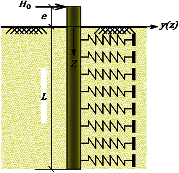
Figure 1: Illustration of pile–soil system using Winkler model
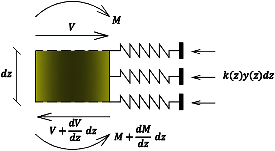
Figure 2: Forces acting in differential pile element
Assuming all forces acting horizontally and applying equilibrium conditions leads to
According to that,
Summation of moments about axis at end of element yields
The relation between bending moment and the shear force is given by
Differentiating Eq. (4) with respect to z and substituting it into Eq. (2) provide
The basic moment-curvature relationship of elementary pile can be written as
The differential equation of a laterally loaded pile can take the form
where
Assuming a linear variation of soil stiffness with soil depth, k can be written as follows [29]
where here
Eqs. (7) and (8) yield
The solution of Eq. (9) requires an iterative procedure to achieve convergence of the relative stiffness factor T as follows [30]
Defining a dimensionless variable
By substituting Eq. (10) into Eq. (11), the governing equation for the soil-pile system is rewritten the form
As shown in Fig. 3, the solution of Eq. (12) requires boundary conditions to balance the number of equations and the number of unknowns.
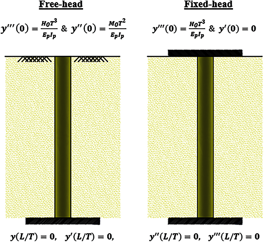
Figure 3: Boundary conditions for the pile under consideration
Boundary conditions of infinitely long piles fixed at the bottom can be written as
The boundary conditions at the top of the pile depend on the circumstances of the lateral deflection, slope, bending moment and shear force. These are generalized into the following two categories.
The pile head is not restrained against rotation and translation. Therefore, the boundary conditions at the pile head can take the form
The pile head is completely restrained against rotation. The boundary conditions at the pile head are given by
Orthogonal systems play a vital role in performing mathematical analysis. This can be due to functions belonging to very general classes can be expanded in series of orthogonal functions e.g., Fourier-Bessel series, Fourier series, etc. Orthogonal polynomials of degree n,
with the orthogonality on the interval
Lemma [32]: If the arbitrary constants
and
where
and
Theorem: If the arbitrary constants k, l, q and m are positive integers, then
and
where
Proof. By using the given lemma and Eq. (17), the theorem is proved.
To solve Eq. (12), the solution domain of our problem must be changed from the interval
So, Eq. (12) could be rewritten as
subject to the conditions of free-head pile
Moreover, the conditions of fixed-head pile are:
The solution of Eq. (25) subject to the conditions given in Eqs. (26) or (27) is written in finite expansion of shifted Legendre function as
Reducing Eq. (25) is performed by orthogonalizing the residual with respect to the basic functions as follows
where the inner product
By substituting Eq. (28) into Eq. (29), a discrete system of
In this case, the vector
The linear system in Eq. (31) is solved using one of the available numerical techniques. By obtaining the coefficients values of
By using the inverse linear transformation
and
In this case, the vector
By using the inverse linear transformation
and
5 Runge-Kutta Formulas of Order 4 and 5 (RKBS45)
The differential equation of laterally loaded pile, Eq. (12), subjected to the boundary conditions in Eqs. (14) or (15) is converted into a system of linear first-order differential equations as follows
If the pile top condition is a free-head one, then the system of equations given in Eq. (39) is subjected to the initial conditions
where the constants
On the other hand, if the pile top condition is a fixed-head one, then the system of equations given in Eq. (39) is subjected to the initial conditions
where the constants
The system of equations Eq. (39) can be rewritten in the vector form as
where
To obtain local error estimates for adaptive step-size control effectively, consider two Runge-Kutta formulas of different orders p and
where s is the number of stages and,
Considering
The solution
The error between the two numerical solutions
In case of
The adapted step size is used to estimate the new values of
6 Validation of the Proposed Methods
The performance and capability of the proposed methods to predict the behavior of laterally loaded piles in cohesion1ess soil have been demonstrated by comparing the obtained numerical results and the observed results from field experiments in full-scale lateral load tests reported by Cox. et al. [33]. In these tests, the flexible free-head steel tube pipe pile of 0.61 m in diameter, 21 m in length, 9.525mm in wall thickness and 163000 kN⋅m2 bending rigidity, was embedded in a deposit of submerged sand. The soil profile at the site is composed of a uniformly fine-graded sand with internal angle of friction,
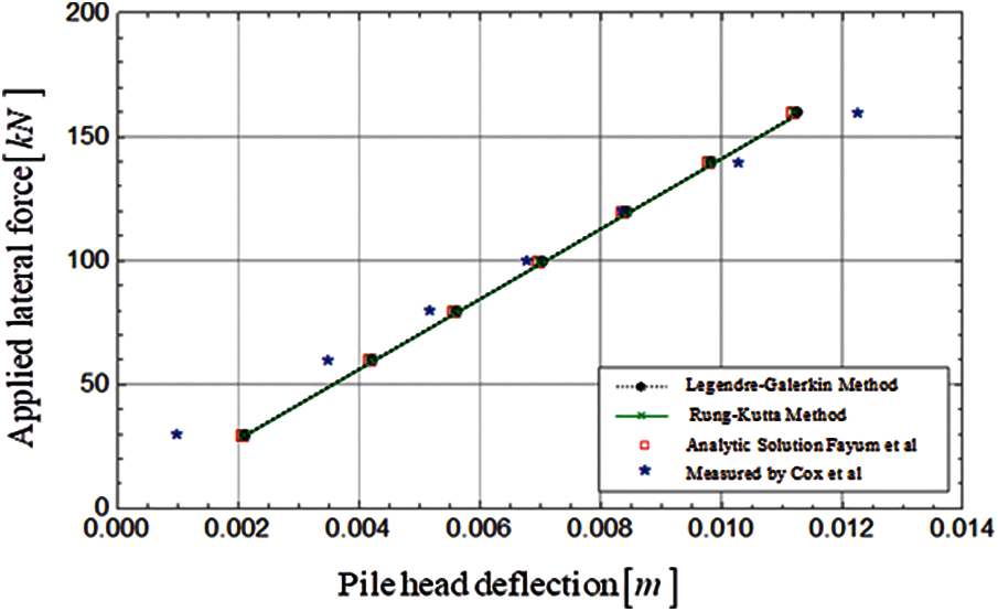
Figure 4: Comparison between the numerical, analytical and experimental lateral deflections of pile head vs. applied lateral force
The design of pile foundation under lateral loads is extensively bound to study both the pile head deflection and the maximum bending moment. Legendre-Galerkin method and Runge-Kutta formulas of order four and five were employed to solve the flexural equation of long piles embedded in homogeneous cohesionless soil with a modulus of subgrade reaction increases linearly with depth. In the numerical simulation, the pile is subjected to horizontal force
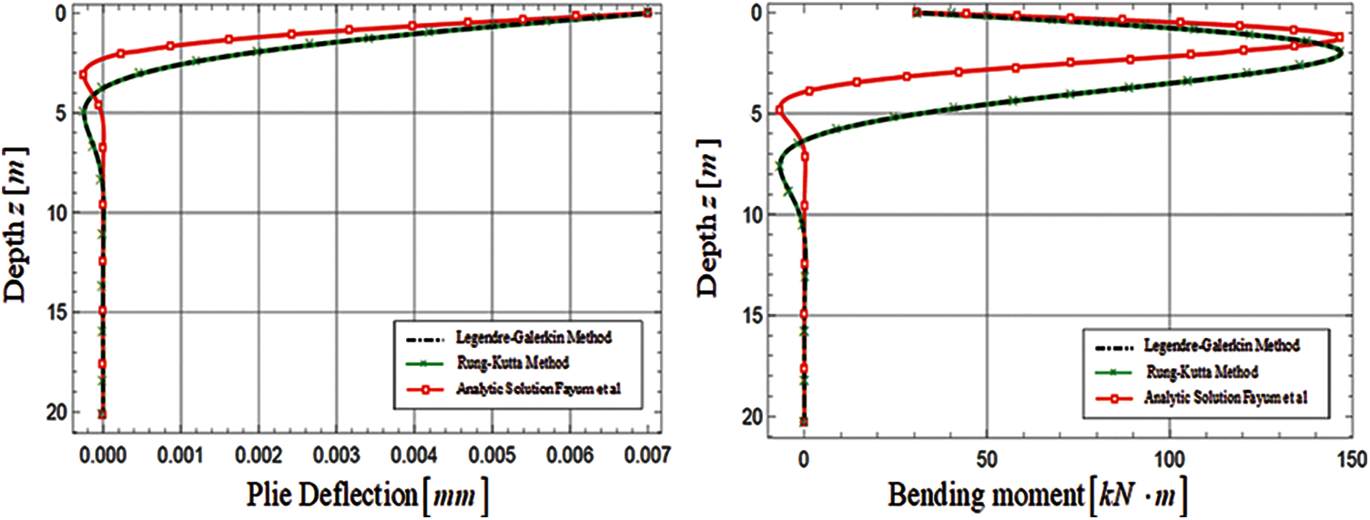
Figure 5: Pile deflection and bending moment profiles of free-head long pile
The plotted curves reveal complete overlaps between Legendre-Galerkin solution and Runge-Kutta solution. Furthermore, the comparison charts demonstrate a very good agreement between the numerical results estimated via Legendre-Galerkin and Runge-Kutta and the corresponding procedure introduced by Fayun et al. [11]. These observations suggest that the lateral deflection and bending moment profiles can be represented accurately by the proposed method. However, insignificant differences between the location of peak deflection and bending moment from proposed methods and solution proposed by Fayun et al. can also be observed regardless the type of head condition.
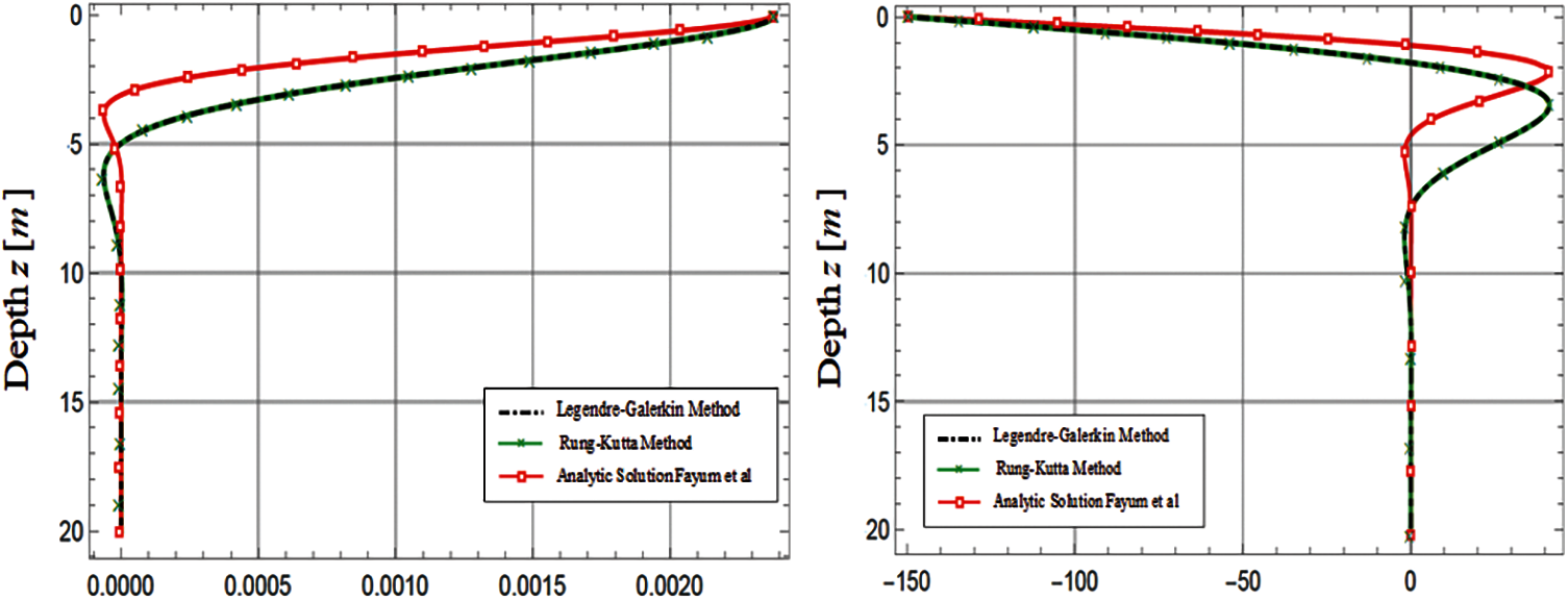
Figure 6: Pile deflection and bending moment profiles of fixed-head long pile
In the present study, Legendre-Galerkin and Runge-Kutta formulas of order four and five methods have been introduced to obtain simplified numerical approaches for understanding the behaviour of single piles against lateral loads. For the purpose of analysis and design of laterally loaded piles crossing sandy soil, simple expressions for the pile lateral deflection and bending moment can be evaluated. The procedure is programmed with the most computational software program Mathematica, which is considered as the world's leading computational software. The numerically computed pile responses are compared with the results from the full-scale lateral load tests. The proposed approaches are well validated. Moreover, these proposed approaches provide evidence that high precision can be achieved with a small amount of computational work. It has been found from the study that the Legendre-Galerkin solution almost coincides with the Runge-Kutta solution for both free-head and fixed-head piles. The suggested numerical expressions obtained in this study can be reasonably applied to analyze and design laterally loaded long piles conveniently. In addition, these techniques can also modify to design/analyze laterally loaded long piles in soil with the modulus of subgrade reaction in any functions of the depth. The proposed approaches capture the long pile behaviour. Furthermore, the proposed solutions are aimed at providing an effective and convenient method for engineers to predict the responses of the entire pile length under the applied lateral load.
Funding Statement: The authors received no specific funding for this study.
Conflicts of Interest: The authors declare that they have no conflicts of interest to report regarding the present study.
1. A. Chore, R. Ingle and V. Sawant, “Parametric study of laterally loaded pile groups using simplified FE models,” Coupled Systems Mechanics, vol. 1, no. 1, pp. 1–7, 2012. [Google Scholar]
2. A. Mostofi and K. Bargi, “Analytical and numerical evaluation of flexible response of floating piers to ship berthing impact,” International Journal of Structural and Civil Engineering Research, vol. 2, no. 1, pp. 249–259, 2011. [Google Scholar]
3. H. Matlock and C. Reese, “Generalized solutions for laterally loaded piles,” Journal of the Soil Mechanics and Foundations Division, vol. 86, no. 5, pp. 63–91, 1960. [Google Scholar]
4. M. Heidari, M. Jahanandish, H. El Naggar and A. Ghahramani, “Nonlinear cyclic behavior of laterally loaded pile in cohesive soil,” Canadian Geotechnical Journal, vol. 51, no. 2, pp. 129–143, 2014. [Google Scholar]
5. D. Su and Y. Zhou, “Effect of loading direction on the response of laterally loaded pile groups in sand,” International Journal of Geomechanics, vol. 16, no. 2, pp. 1–12, 2016. [Google Scholar]
6. D. Su and J. Li, “Three-dimensional finite element study of a single pile response to multidirectional lateral loadings incorporating the simplified state-dependent dilatancy model,” Computers and Geotechnics, vol. 50, no. 5, pp. 129–142, 2013. [Google Scholar]
7. S. Gleser, “Lateral load tests on vertical fixed-head and free-head piles,” Symp. on Lateral Load Tests on Piles, ASTM STP, vol. 154, pp. 75–101, 1953. [Google Scholar]
8. M. Ashour and G. Norris, “Modelling lateral soil-pile response based on soil-pile interaction,” Journal of Geotechnical and Geoenvironmental Engineering, vol. 126, no. 5, pp. 420–428, 2000. [Google Scholar]
9. Z. Moayed, A. Judi and B. Rabe, “Lateral bearing capacity of piles in cohesive soils based on soil's failure strength control,” Electronic Journal of Geotechnical Engineering, vol. 13(Dpp. 1–11, 2008. [Google Scholar]
10. Y. Chang, “Discussion on lateral pile loading tests,” L.B. Feagin. Trans. ASCE, vol. 102, pp. 272–278, 1937. [Google Scholar]
11. L. Fayun, L. Yanchu, L. Lei and W. Jialai, “Analytical solution for laterally loaded long piles based on Fourier-laplace integral,” Applied Mathematical Modelling, vol. 38, pp. 5198–5216, 2014. [Google Scholar]
12. E. Conte, A. Troncone and M. Vena, “Nonlinear three-dimensional analysis of reinforced concrete piles subjected to horizontal loading,” Computers and Geotechnics, vol. 49, pp. 123–133, 2013. [Google Scholar]
13. S. Gleser, “Lateral load tests on vertical fixed-head and free-head piles,” Symp. on Lateral Load Tests on Piles, ASTM STP, vol. 154, pp. 75–101, 1953. [Google Scholar]
14. P. Ruesta and F. Townsend, “Evaluation of laterally loaded pile group at roosevelt bridge,” Journal of Geotechnical and Geoenvironmental Engineering, vol. 123, no. 12, pp. 1153–1161, 1997. [Google Scholar]
15. D. Brown, L. Resse and M. O'Neill, “Cyclic lateral loading of a large-scale pile group,” Journal of Geotechnical Engineering, vol. 113, no. 11, pp. 1326–1343, 1987. [Google Scholar]
16. S. Yousefi, “Legendre wavelets method for solving differential equations of lane-emden type,” Applied Mathematics and Computation, vol. 181, pp. 1417–1422, 2006. [Google Scholar]
17. J. Shen, “Efficient spectral-galerkin method i. direct solvers for second- and fourth-order equations by using legendre polynomials,” SIAM Journal on Scientific Computing, vol. 15, pp. 1489–1505, 1994. [Google Scholar]
18. X. Ye, “The legendre collocation method for the cahn-hilliard equation,” Applied Mathematical Modelling, vol. 150, pp. 87–108, 2003. [Google Scholar]
19. A. Khater, A. Shamardan, D. Callebaut and M. Sakran, “Numerical solutions of integral and integro-differential equations using legendre polynomials,” Numerical Algorithms, vol. 46, pp. 195–218, 2007. [Google Scholar]
20. B. Bialecki and A. Karageorghis, “Legendre gauss spectral collocation for the helmholtz equation on a rectangle,” Numerical Algorithms, vol. 36, pp. 203–227, 2004. [Google Scholar]
21. W. Zhengsu, C. Yanping and H. Yunqing, “Legendre spectral galerkin method for second-kind volterra integral equations,” Frontiers of Mathematics in China, vol. 4, pp. 181–193, 2009. [Google Scholar]
22. M. Fathy, M. El-Gamel and M. El-Azab, “Legendre-galerkin method for the linear fredholm integrodifferential equations,” Applied Mathematics and Computation, vol. 243, pp. 789–800, 2014. [Google Scholar]
23. S. Yousefi, “Numerical solution of abel's integral equation by using legendre wavelets,” Applied Mathematics and Computation, vol. 175, pp. 574–580, 2006. [Google Scholar]
24. P. Bogacki and L. Shampine, “An efficient runge-kutta (4, 5) pair,” Computers & Mathematics with Applications, vol. 32, pp. 15–28, 1996. [Google Scholar]
25. E. Elbashbeshy, T. Emam, M. El-Azab and K. Abdelgaber, “Effect of thermal radiation on flow, heat and mass transfer of a nanofluid over a stretching horizontal cylinder embedded in a porous medium with suction/injection,” Journal of Porous Media, vol. 18, no. 3, pp. 215–229, 2015. [Google Scholar]
26. E. Elbashbeshy, T. Emam, M. El-Azab and K. Abdelgaber, “Slip effect on flow, heat, and mass transfer of a nanofluid over a stretching horizontal cylinder in the presence of suction/injection,” Thermal Science, vol. 20, no. 6, pp. 1813–1824, 2016. [Google Scholar]
27. A. Hanna and A. Sharif, “Drag force on a single pile in clay subjected to surcharge loading,” International Journal of Geo-Mechanics, ASCE, vol. 6, no. 2, pp. 89–99, 2006. [Google Scholar]
28. L. Xu, F. Cai, G. Wang and K. Ugai, “Nonlinear analysis of laterally loaded single piles in sand using modified strain wedge model,” Computers and Geotechnics, vol. 51, pp. 60–71, 2013. [Google Scholar]
29. H. Poulos and E. Davis, Pile Foundation Analysis and Design, New York: Wiley, 1980. [Google Scholar]
30. L. Reese and H. Matlock, “Non-dimensional solutions for laterally loaded piles with soil modulus assumed proportional to depth,” in Proc. of the 8th Texas Conf. on Soil Mechanics and Foundation Engineering, Austin, TX, pp. 1–23, 1956. [Google Scholar]
31. N. Lebedev and R. Silverman, Special Functions and Their Applications, New York: Dover Publications, 1972. [Google Scholar]
32. E. Doha, “On the construction of recurrence relations for the expansion and connection coefficients in series of jacobi polynomials,” Journal of Physics A: Mathematical and Theoretical, vol. 37, no. 3, pp. 657, 2004. [Google Scholar]
33. W. Cox, L. Reese and B. R. Grubbs, “Field testing of laterally loaded piles in sand,” in Proc. of the 6th Annual Offshore Technology Conf., Houston, TX, Paper No. OTC 2079, vol. 2, pp. 459–472, 1974. [Google Scholar]
34. R. Liang, “Drilled shaft foundations for noise barrier walls and slope stabilization,” Final Report, FHWA/OH-2002/038, Ohio Department of Transportation, OH, 2002. https://www.semanticscholar.org/paper/Drilled-Shaft-Foundations-for-Noise-Barrier-Walls-Liang/0399dd8a66a13b23de4e984975569f89b17a5e4d [Google Scholar]
 | This work is licensed under a Creative Commons Attribution 4.0 International License, which permits unrestricted use, distribution, and reproduction in any medium, provided the original work is properly cited. |