Computers, Materials & Continua DOI:10.32604/cmc.2022.022183
Article

Path Planning Based on the Improved RRT* Algorithm for the Mining Truck

Dong Wang1,*, Shutong Zheng1, Yanxi Ren2 and Danjie Du3

1School of Instrument Science and Engineering, Southeast University, Nanjing, 210096, China
232184 PLA Troops, Beijing, 100071, China
3North Carolina State University, Raleigh, USA
*Corresponding Author: Dong Wang. Email: kingeast16@seu.edu.cn
Received: 30 July 2021; Accepted: 09 October 2021

Abstract: Planning a reasonable driving path for trucks in mining areas is a key point to improve mining efficiency. In this paper, a path planning method based on Rapidly-exploring Random Tree Star (RRT*) is proposed, and several optimizations are carried out in the algorithm. Firstly, the selection process of growth target points is optimized. Secondly, the process of selecting the parent node is optimized and a Dubins curve is used to constraint it. Then, the expansion process from tree node to random point is optimized by the gravitational repulsion field method and dynamic step method. In the obstacle detection process, Dubins curve constraint is used, and the bidirectional RRT* algorithm is adopted to speed up the iteration of the algorithm. After that, the obtained paths are smoothed by using the greedy algorithm and cubic B-spline interpolation. In addition, to verify the superiority and correctness of the algorithm, an unmanned mining vehicle kinematic model in the form of front-wheel steering is developed based on the Ackermann steering principle and simulated for CoppeliaSim. In the simulation, the Stanley algorithm is used for path tracking and Reeds-Shepp curve to adjust the final parking attitude of the truck. Finally, the experimental comparison shows that the improved bidirectional RRT* algorithm performs well in the simulation experiment, and outperforms the common RRT* algorithm in various aspects.

Keywords: RRT*; optimize; path smooth; coppeliaSim

1  Introduction

Mineral resources, as the most important raw materials for industrial production, have become a top priority for research in various countries on how to mine them efficiently and intelligently. Some developed countries have conducted much research and development on “unmanned mines” [1–3]. The Canadian government's “Plan 2050” plans to transform the distant northern mines into smart mines. Finland, Sweden and other Nordic countries have also done some in-depth research in the field of mining equipment automation [4], and Australia was the first country that initiated the research on unmanned trucks [5]. As a medium for transporting materials, mining trucks are the top priority for realizing smart mines. Therefore, the unmanned mining area construction is the future trend, and the main technical difficulty lies in how to plan a suitable driving path for the mining truck in a complex environment, both to identify passable roads and to satisfy the movement characteristics of mining trucks, as well as the efficiency of the path.

In terms of this difficulty, many scholars have made numerous researches. First of all, to simulate the movement of the real vehicle, a kinematics model of the vehicle needs to be established. Some scholars have constructed the anti-skid model of the unmanned mining truck based on kinematics geometry and two different models considering the slip through the Kalman filter. Others proposed Ackermann steering model to solve the problem of vehicle kinematics steering in simulation, and modeling research based on Ackermann steering principle became mainstream. At the same time, vehicle path planning is one of the most classic optimization problems in the field of operational research optimization, and there are many algorithms. The common path planning methods include A*, D*, Dijkstra, Rapidly-exploring Random Tree (RRT), artificial potential field algorithm and so on [6–9]. Among them, the RRT algorithm [10] was proposed by Steven M Lavalle, which has the advantages of no need to model the space and having an absolute solution, but also has the defects of the unguided search process and low efficiency. To overcome these shortcomings, some scholars proposed the MI-RRT* algorithm [11] based on the RRT* algorithm [12]. This algorithm improves the RRT* algorithm through four modules: target bias model, dynamic compensation, limiting the number of RRT* nodes, and elliptical sampling. Based on these, some researchers established an environmental grid model based on GIS map of mine and solved the global path planning problem of intelligent truck with improved ant colony algorithm [13]. Some proposed an improved asymptotically optimal RRT algorithm based on goal-biased constrained sampling and goal-biased extending to improve the efficiency of path planning [14].

The research on kinematic modeling and path planning algorithms in the field of smart cars and unmanned vehicles has made great progress in recent years. However, the research on the connection between them is still lacking. The research on establishing and improving the kinematics model supported by the corresponding path planning algorithm mainly belongs to the field of robotics, and in field of vehicle simulation, most studies only uses simple differential rotation models or only simple geometry instead, and although the structure of such models is low in difficulty, the gap with the models of real vehicles is large. To this extent, the study lacks practical guidance.

In this paper, an improved bidirectional RRT* algorithm is proposed for the path planning of mining trucks. The optimization process and path smoothing process in the improved algorithm will be introduced in the second part. The third part is the experimental part. The superiority of the algorithm proposed in this paper is verified by comparing RRT* and the improved bidirectional RRT* on the same map and by comparing metrics such as running time, total number of iterations and successful expansion points. Finally, a truck model is built in CoppeliaSim to carry out the simulation experiment.

2  RRT* Optimization Method

In order to find the truck's travel path in a complex mining environment, an improved bidirectional RRT* algorithm is proposed. The algorithm is optimized and improved on the RRT* proposed by Sertac and Emilio at MIT. It is mainly optimized in the following process: (1) the selection process of the growing target point is optimized by handing over the original random points and trying to grow toward the target point; (2) the process of selecting the parent node is optimized by including the distance from the tree node to the target point in the measurement, and the Dubins [15,16] curve is used for constraint, so that the obtained path is more realistic; (3) The expansion process from tree nodes to random points is optimized by the gravitational repulsion field method and dynamic step size method; (4) Dubins curves are used in the obstacle detection process to ensure that the obtained paths are larger than the minimum turning radius of the vehicle. In order to speed up the iteration speed, this paper finally chooses to use bidirectional RRT*. And the greedy algorithm and cubic B-spline interpolation are used to smooth the path to reduce the length of the path respectively.

2.1 Optimization in Random Sampling

The generation of random points in the original RRT* algorithm is completely random without intervention and lacks guidance, which will lead to a large amount of computation. The optimization idea adopted in this paper is that, given the probability threshold p, a random number q (0∼1 random distribution) is generated before each generation of random points. If q < p, then Xgoal(final target point) is used as the growth target point for the child nodes of the extension tree, and vice versa, Xrand (random generation point) is used as the growth target point. The purpose of this method is to make the random extended tree grow to the final target point and improve the computational efficiency. Since the RRT* algorithm in this paper is applicable to vehicle path planning [17], a ternary RRT algorithm should be adopted, that is, in addition to (x,y) coordinates, direction parameter θ, and the generation of direction parameter also needs to be optimized. This idea is different from the random generation of coordinates, which is as follows: Given that the direction Angle of the vector XinitXgoal→ as θ0, the probability function is adopted as the normal distribution function, μ=θ0, 2σ=90∘. According to the 3σ principle, it can be known that for the random direction parameter θrand: The probability of θrand:θ0−90∘<θrand<θ0+90∘ is about 95.4%. This is because it is difficult for the vehicle to deviate from the direction of ±90∘ during the process from the start point to the end point, and in such a direction it is easy to reduce the overall algorithm efficiency due to the failure of obstacle detection.

2.2 Parent Node Selection Optimization

In the basic RRT* algorithm, the nearest tree node Xnearest is measured by the Euclidean distance from the random point to the tree node Xtree. The optimization idea proposed in this paper is to include the distance between tree node and the final goal point Xgoal into the measurement range:

distance=Ci∗||Xrand−Xtree||+Cj∗||Xgoal−Xrand||(1)

Considering these two factors, the random tree [18] will approach to the end point in a “leading” way.

The concept of Dubins curve is introduced here. The Dubins curve takes into account the effect of turning radius on the motion of a vehicles or an aircraft and finds the shortest path curve between the initial and termination states of the object by geometric analysis [19]. In this paper, in addition to obstacle detection by Dubins curve, it is also applied to the process of obtaining the nearest tree node as discussed above. Because Ackermann vehicle has a minimum turning radius in actual motion, the Euclidean distance is not the shortest in the pratical sense, as shown in Fig. 1, the current vehicle state is a solid rectangle with three alternative targets shown as dashed lines, now the aim is to find the nearest target for the current vehicle, if only the Euclidean distance is considered, then there is no doubt that the first case is the closest with a Euclidean distance of 0 and the second case is the second. However, for the Ackerman car, in-situ steering and lateral translation are not possible due to the minimum turning radius, so in fact, the third case is the “closest” vehicle.

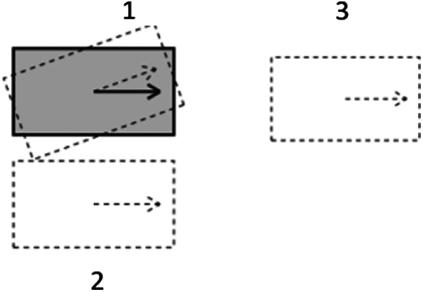
Figure 1: Different target attitude

Therefore, Eq. (1) is modified like this:

distance=Ci∗length(Dubins)+Cj∗||Xgoal−Xrand||(2)

In this paper, only the first term in Eq.(2) is changed to the Dobbins curve length, the reason is that during most of the algorithm running time, the distance between the target point and the random point is very large, and the difference between the Dobbins curve length and the Euclidean distance is very small, which is only obvious at the end, for this reason, the improved RRT* algorithm in this paper finally adopts a bidirectional RRT* algorithm, that is, to generate two trees from the starting point and the end point respectively random expansion trees. As a result, the apparent gap between the length of the Dobbins curve and the Euclidean distance near the end point is eliminated. In addition, the second term still retains the Euclidean distance from the target point to the random point, considering that replacing the Dobbins curve increases the computational effort.

2.3 Optimization of Tree Node to Random Point Expansion Process

The expansion from the nearest tree node to the random point is the core of the improved bidirectional RRT* algorithm, as shown in Fig. 2. In this paper, the gravitational repulsive force field method and dynamic step size method are used for optimization.

The artificial potential field method [20] introduces the idea of gravitational and repulsive forces similar to the electric potential field into the path planning algorithm. In the RRT* algorithm, the target point can be regarded as the gravitational field and the obstacle as the repulsive force field. In this way, the randomly expanding tree will move away from the obstacle while tending to expand towards the target, and the magnitude of this trend depends on the correlation coefficient, as shown in Fig. 3.

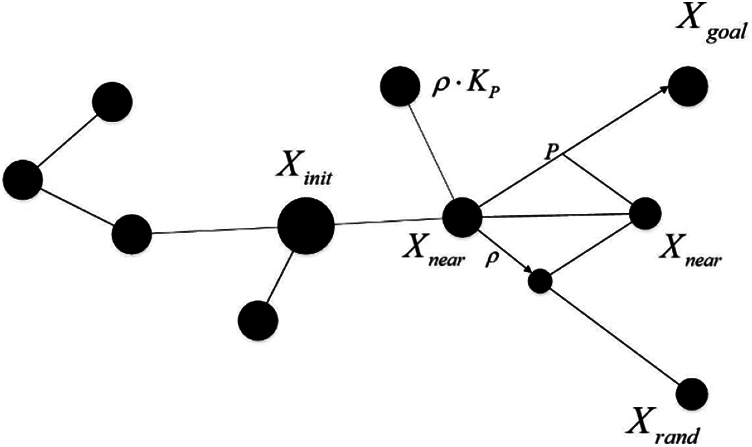
Figure 2: The expansion of tree nodes to random points after adding the gravitational potential field

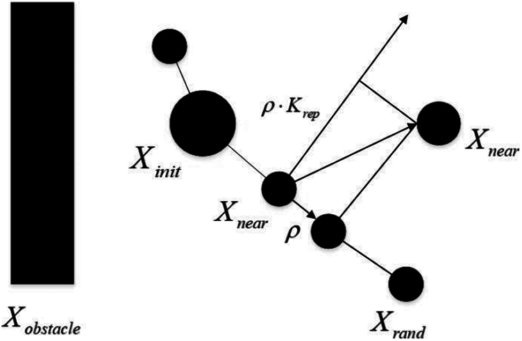
Figure 3: The expansion of tree nodes to random points after adding the repulsive potential field

Assume that the expension step of the RRT* algorithm is ρ, the gravitational coefficient is KP, and the random growth function G(n) does not add the gravitational potential field:

G(n)=ρXrand−Xnear||Xrand−Xnear||(3)

Referring to the common gravitational potential function model, where ς is scale factor, d(q,qgoal) represents the distance between the object and the target:

Uatt(q)=12ςd2(q,qgoal)(4)

Add a target gravitational function R(n):

R(n)=ρ∗KpXgoal−Xnear||Xgoal−Xnear||(5)

Referring to the common repulsive potential field function model:

Urep(q)={12η(1D(q)−1Q∗)2,D(q)≤Q∗0,D(q)>Q∗(6)

This paper proposed a target repulsion function T(n):

T(n)={0,p(x)>p0ρ∗krep∗(1p(x)−1p0)2xnear−xobstacle||xnear−xobstacle||,p(x)≤p0(7)

After adding the gravitational field and repulsive potential fields, the random growth function is F(n)=G(n)+R(n)+T(n). In this paper, the action range of the repulsive potential field P0 needs to be modified, and the obstacle Xobstacle has three parameters (x,y,d0). d0 is the expansion distance of the obstacle. Considering that the actual vehicle has a certain width, it is necessary to keep a certain distance between the obstacles and the driving route. It is assumed that the original influence range of the repulsive potential field of the obstacle is Pinit, and after considering the expansion distance, P0=D0+Pinit.

At the same time, the algorithm is optimized by dynamically extended step size ρdynamic. In the original RRT* algorithm, if the fixed step size is set too small, the random tree will grow slowly. If the step size is set too large, it tends to make the new nodes difficult to expand in dense obstacle areas and the overall efficiency of the algorithm decreases. The dynamic step size strategy is as follows: Di is the nearest distance from Xnearest to the expansion obstacle and ρmin and ρmax are the upper and lower bounds of the step size.

For step size ρ:

ρ={ρmax,Di>ρmaxDi,ρmin⩽Di⩽ρmaxρmin,Di<ρmin(8)

When the distance from the obstacle is far, the upper limit of step size is adopted. Compared with the traditional fixed step size, the dynamic step size can accelerate the growth of random tree in open areas. When near an obstacle, the fixed-step transmission often fails to pass the obstacle detection, falling to generate new tree nodes, which will also reduce the growth rate of the random tree. If the dynamic step size is adopted, this problem can be well solved due to its adaptability. Using dynamic step size can greatly improve the success rate of new node generation and effectively improve the overall algorithm efficiency.

2.4 Optimization of Obstacle Detection Process

The idea of RRT* algorithm or most RRT deformation algorithms in obstacle detection is basically to take a certain numerical sampling point Xlist at line XnearXnew, traversal the nearest distance between all points of Xlist and the obstacle, and obtain the nearest distance dmin. If dmin>d0 (d0 is obstacle expansion distance), it means that obstacle detection has passed and Xnew has been successfully placed in the random tree.

Since the research object is an Ackermann vehicle, and all points have directional parameters, the constraint of the minimum steering radius of the Ackermann vehicle will be ignored if only the line XnearXnew is sampled. Therefore, this paper proposes to use Dubins curve for obstacle detection. The turning radius parameter should be obtained when generating the Dubins curve. After repeating tests and analysis, it is concluded that the minimum turning radius Rmin of the vehicle should not be taken directly because the vehicle may not reach the maximum turning angle when turning in actual driving, which means that the turning radius of the vehicle is greater than the minimum turning radius in most cases. So the radius parameter in the Dubins curves generating function should be slightly bigger than Rmin, the specific value can be judged according to the demand, and if the radius solution is large, the path obtained is more “safe”. However, a larger radius also trends to cause failure to pass obstacle collision detection, resulting in a decrease in the overall efficiency of the algorithm, so it needs to compare experiments many times, obtain a radius value that balances algorithm efficiency and path safety. So several experiments are needed to obtain a radius value that balances the efficiency of the algorithm and path safety. The rest of the process is consistent with the basic RRT* algorithm. In general, the sampled paths are modified, which increases the computational effort to some extent, but the paths generated by Dubins curves are more practical.

2.5 Path Smoothing Algorithm

2.5.1 Pruning Based on Greedy Algorithm

The main idea of the Greedy algorithm is to divide the solved problem into several subproblems and ask for the local optimal solution of each subproblem without considering the global one. Finally, the optimal solutions of each subproblem is superimposed to obtain the final solution.

The pruning process using greedy algorithm in this paper is as follows:

(1). Given that the set of Path points obtained by the RRT* algorithm Path, it can be known by referring to the idea of greedy algorithm that the local problem should be set first. In the pruning process of RRT* algorithm, the local problem is to find the Dubins curve path from Path[n] to Path[n + C](C is the preset constant) that can pass obstacle detection. The path Dubins curve found is from Path[n] to Path[n + d] and the range of d is from 0 to C.

(2). Given dmax, the maximum number of d that can pass obstacle detection from Path[n] to Path[n + d].

(a). If dmax≠0, Dubins curves are directly established from Path[n] to Path[n + dmax] and the original curves are deleted. If Path[min(n + C,n + dmax)] is the end point, then the algorithm stops and outputs the path; otherwise, Path[min(n + C,n + dmax)] is taken as the starting point of the next traversal.

(b). If dmax=0, it means that no pruning can be done, and the original path is already the best, then all the original path curves from Path[n] to Path[n + d] are retained. If Path[n + dmax] is the end point, then the operation is aborted and the path is printed. Otherwise, Path[n + dmax] is taken as the starting point for the next traversal. The key point to pruning operation in this paper is the selection of C, that is, how to define the local problem. From many studies, it is more appropriate to take C as the 25% of the original number of the paths.

It is easy to find that the pruned path is still not optimal, which is determined by the nature of the greedy algorithm, as it can only produce a local optimal solution, if a smaller number of final path points and a smoother path are needed, it is necessary to increase the C (the traversal times under local problem), but the computation will be larger, so it is very important to balance these two points.

After pruning, the overall smoothing effect is obvious. However, the smoothing effect still needs further improvement for real vehicles due to the randomness of the direction parameters and the presence of the Dobbins curve constraint. Therefore, the cubic B-spline interpolation method is introduced as the second step of path smoothing.

2.5.2 Path Smoothing Based on Cubic B-Spline Interpolation

The advantage of B-spline interpolation is that it does not change the overall shape of the path significantly and only deals with the tortuous phenomena in a small range locally. Given that there are currently c + 1 points, the model of the cubic B-spline curve is as follows:

Ck(u)=∑i=0Pi+kBi,3(u),u∈[0,1),k=0,1,…,c−3(9)

For Bi,3(u), there are:

B0,3(u)=(−u3+3u2−3u+1)/3!B1,3(u)=(3u3−6u2+4)/3!B2,3(u)=(−3u3+3u2+3u+1)/3!B3,3(u)=u3/3!(10)

A key parameter S in the algorithm defaults to 0, which represents the smoothness of the curve after interpolation. The larger S is, the smoother the curve will be. The selection of S is the key factor in the success of path smoothing. Assuming S = 0, the interpolated curve is not much different from the original path curve and smoothing has no effect. However, the S is not as larger as better. If the S is too large, the interpolated curve will seriously “deviate” from the original curve, causing the curve to intersect with the obstacle and leading to the failure of vehicle path planning. Therefore, the setting of S requires several attempts to obtain a relative optimal solution.

Referring to the idea of Greedy algorithm principle, a dynamic S-parameter algorithm is proposed and the specific procedure is as follows:

(1). Sampling on the smoothed curve Pathsmooth, the specific sampling points need to be adjusted according to the actual situation, and the obstacle detection is conducted on the sampling points in turn.

(2). If the obstacle detection passes, the final path is Pathsmooth, S is substituted with S-C (C is the default constant) and then substituted into B-spline interpolation. Then Step one is carried out again until the obstacle detection passes. Here, C should be determined according to the actual demand. If a smoother path is wanted, C should be smaller, but this will reduce the efficiency of the operation. If the algorithm efficiency is more important, C should be appropriately large.

3  Analysis and Discussions of Experiment Result

3.1 Performance of the Improved Bidirectional RRT* Algorithm

The evaluation indexes of improved bidirectional RRT* are as follows: running time, total iteration times, number of successful expansion points and path length. This paper used the map to test the improvement of the improved bidirectional RRT* algorithm over the original algorithm in different states. Firstly, the point (30, 90) was chosen as the starting point and (480, 480) was chosen as the end point. The results obtained by using the basic RRT* algorithm are shown in Fig. 4:

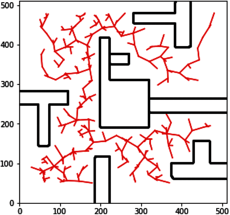
Figure 4: Result of the basic RRT* algorithm

Then, the improved bidirectional RRT* algorithm was verified as shown in the following figure. In Fig. 5a, the specific parameters of the algorithm were as follows: dynamic step size is 40 ± 10, gravitational coefficient Kp=0.1, repulsion coefficient Krep=1, and the coefficient of the effect of the endpoint on the nearest point search Cj=0.02. In Fig. 5b, Kp=1, Krep=1, and the remaining coefficients are the same as those in Fig. 5a. In Fig. 5c, Kp=0.1 and Krep=5, and the other parameters are consistent with the above two cases.

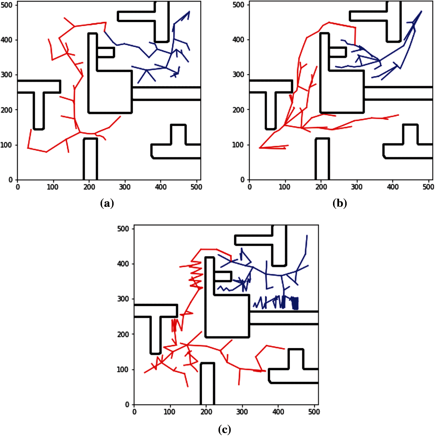
Figure 5: Results of the improved bidirectional RRT* algorithm

First of all, it is obvious that the basic RRT* algorithm lacks target and traverses almost the entire map, and other trees can extend until the two trees intersect. Then, a brief comparison of the three cases of the improved bidirectional RRT* algorithm is made. In terms of commonality, they are superior to the ordinary RRT* algorithm in terms of both the number of iterations and time consumption. Fig. 5a belongs to the compromise case, where it can be seen that the extension tree has certain obstacle avoidance and target tendency, but neither is obvious. Fig. 5b belongs to the dominant gravitational field at the target point, which is the target point extending the tree branches under the dominant gravitational field. In general, the direction of the branch is considered irregular, but in Fig. 5b, most branches are oriented towards the target, in another word, the branches are attracted by the target point. The advantage of the gravitational field is that when it dominates, the expansion of the tree can be limited in a certain area, and a small search area will help improve the search efficiency. But when there are obstacles in the search range, as shown in this example, the overall efficiency of the algorithm becomes low, as the data analysis clearly illustrates. In some cases, the presence of a gravitational field can even cause a negative optimization. Finally, the situation in Fig. 5c shows the extremes situation of repulsive force field, it can be seen that when tree nodes are close to the obstacles, the expansion of the tree node will deviate from the obstacles due to the repulsive force of the obstacle. Although the repulsion parameters is large, the path searching process is very chaotic, it does not affect the overall algorithm, because only the path points for the next pruning are obtained, and it does not matter how these path points are obtained, the whole process only cares about the time and the number of iterations.

In this paper, the data of algorithm time consumption, number of iterations, and standard deviation of running time before and after algorithm optimization at the time of experiments are counted. Fig. 6 shows the comparison of the time consuming of different algorithms. It can be seen from the figure that the time consuming of the improved bidirectional RRT* algorithm is much lower than that of the basic RRT* algorithm, and the time consuming is further shortened after using the process optimization method proposed in this paper.

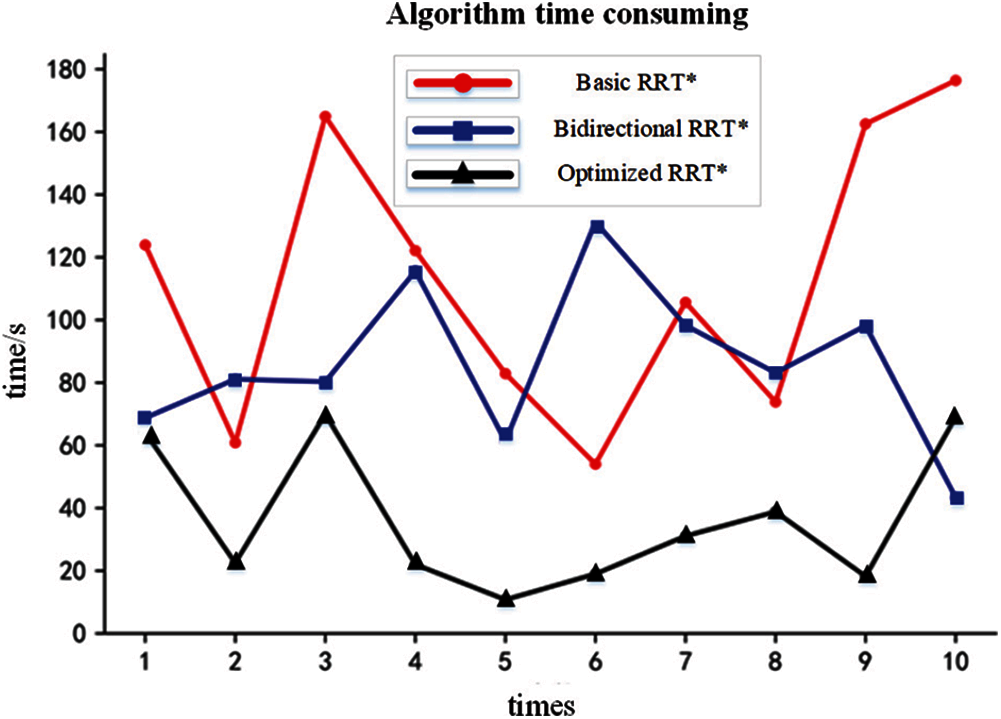
Figure 6: Algorithm time-consuming comparison

As shown in Fig. 7, the basic RRT* has the highest number of iterations, the bidirectional RRT* has the second highest number of iterations, and the improved bidirectional RRT* has the lowest number of iterations.

The parameters of the improved bidirectional RRT* algorithm selected here are the gravitational coefficient Kp=0.2 and the repulsive coefficient Krep=5. It can be seen that from the basic RRT* to the bidirectional RRT* and finally the improved bidirectional RRT*, there is a step-by-step optimization in terms of running time, number of iterations and stability of the algorithm. However, there are also some shortcomings in the algorithm, through the Fig. 7 can be seen that a single iteration time of basic RRT* was about half of that used in bidirectional RRT* and improved bidirectional RRT*, this means that when using two trees to calculate a single iteration, the efficiency is lower and need to optimize the algorithm structure. From another point of view, although the single iteration efficiency of the improved bidirectional RRT* is lower, the optimized RRT* algorithm still brings a huge improvement to the overall efficiency, which further demonstrates the high quality of the algorithm.

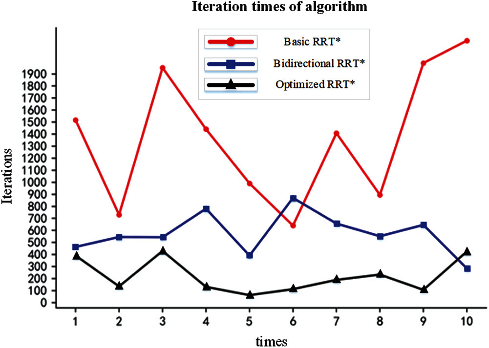
Figure 7: Algorithm iteration times comparison

Due to the efficiency of the optimized algorithm depends highly on the coefficient, such as gravity coefficient, repulsive force coefficient, how to find the right coefficient to improve the algorithm efficiency is a top priority. And then this paper will show the efficiency of the algorithm under several different coefficients to explore each factor's influence on the algorithm and summed up the relevant conclusions. The data in Tab. 1 for each group is based on 10 experiments.

From the situation of the seven test groups, when Krep=5 and Kp=0.2, the average running time is the shortest, the stability is good, and the average iteration number is the best. Generally speaking, this is the best set of parameters in the selected test group. When the gravity coefficient Kp has a big influence, algorithm optimization is not good, even as in the situation mentioned above, the negative optimization occurs. When the gravity coefficient is larger, the algorithm running time of the standard deviation is larger, reflects that the algorithm running time standard deviation is very big, it is worth mentioning that in all test groups, When Krep=3 and Kp=0.5, the shortest time 9.61 s appeared in this group, and the second-longest time 116.86 s also appeared in this group, which fully reflected its instability.

The improvement of algorithms made by the repulsive force coefficient is mainly reflected in the expansion rate, namely, the detection probability through obstacles. As a result of the repulsive force coefficient, some points that cannot pass the obstacle detection can bypass obstacles and eventually achieve the expansion of the tree nodes. The expansion success rate in the data reflects this. And when the expanding success rate is high, the running time standard deviation of the corresponding algorithm is also reduced, and the stability is improved. On the contrary, when the gravity of the target point increases, the success rate of expansion does not improve, but tends to decrease. Therefore, through the comparison of these sets of experiments, this paper obtains the conclusion of optimizing the parameter settings of the RRT* algorithm.

First of all, the selection of the repulsion coefficient should not be too small, because the meaning of the existence of the repulsion force of the obstacle is to keep the point away from it. According to the above tests, Krep=5 is a reasonable value. In the preliminary test, this algorithm found that the influence of the repulsive field was limited. After the study, the repulsive field model established by Eq. (11) was improved to the following situation:

T(n)={0,p(x)>p0ρ∗krep∗(1p(x)−1p0)xnear−xobstacle||xnear−xobstacle||,p(x)≤p0(11)

In the original model, 1p(x)−1p0 adopted the square term so as to be more closed to the general repulsion potential field model. However, in the actual calculation, it is found that in most cases, 1p(x)−1p0 is very small and even close to 0 after the square. Therefore, no matter how large the repulsion coefficient Krep is, the repulsion field will not be affected. Therefore, it is revised.

Secondly, the selection of the gravitational coefficient should be adjusted according to the actual map. Although the gravitational coefficient can cause a certain negative optimization when it is too large, the gravitational coefficient should not be completely discarded. From the two control experiments (Krep=3,Kp=0) and (Krep=3,Kp=0.2), (Krep=5,Kp=0) and (Krep=5,Kp=0.2), the existence of gravitational coefficient is very necessary, especially when Krep is large.

In this paper, the effect of dynamic step size on the algorithm is also tested, the conclusion is that it has little effect on the algorithm speed and it can improve the success rate of expansion to a small extent and improve the overall algorithm stability.

In general, the principle of the optimizing RRT* algorithm for gravity and repulsion algorithm is as follows: the repulsion parameter Krep needs to ensure that the points near the vast majority of close obstacles will not expand toward the obstacle due to the existence of the gravitational force at the target point. Secondly, the size of the gravitational coefficient Krep is needed to ensure that the original expansion path towards to the target point in the open area without the existence of repulsive force to improve the operation efficiency. When the overall map is complex, it is suggested to adopt dynamic step size and decrease the lower limit of step size, which can effectively improve the iteration efficiency.

3.2 Mining Truck Simulation

The 3D terrain and obstacle modeling of the mine site was carried out by Blender software. After importing CoppeliaSim, it was connected to Python and then imported into the algorithm for real-time control. In the simulation environment, as shown in Fig. 8, there are many obstacles, but there is at least one passable road between them. In this section, we conducted path planning simulation experiments by setting different starting points and target points. The top view of the map is shown as follows:

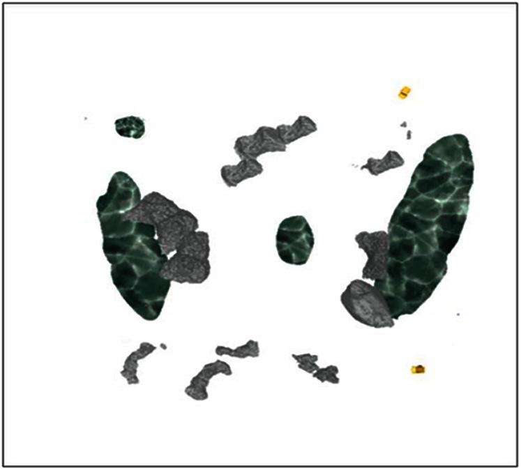
Figure 8: Top view of the simulated mine

The kinematic model of unmanned mining vehicle based on Ackermann's principle uses the Stanley algorithm in optimal preview control to achieve path tracking after obtaining the vehicle path. However, the Stanley algorithm does not consider the Ackermann's geometric steering and always assumes the front wheel steering angle is the same. Therefore, the algorithm needs to be modified to make it compatible with the Ackermann geometric steering. Finally, the paths tracked under the Stanley algorithm can be seen in Fig. 9, with the axes representing the position of each waypoint on the map.

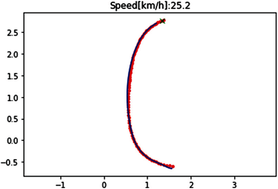
Figure 9: Path under Stanley algorithm

Then, in order to fully validate the robustness of the path planning algorithm for unmanned mining trucks, this section will be carried out multiple times by changing the end point. The specific validation results are as follows. The x and y axes in all of the following graphs represent the coordinate system in the map, and (x, y) represents the coordinates of each point on the map:

Firstly, the car was tested with the bottom right corner of the map as the starting point and the top right corner as the end point. The red line is the pruned path of the Dubins curve, and the blue line is the interpolated smooth path. The test results are shown in Fig. 10.

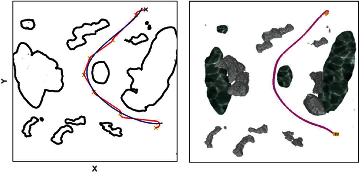
Figure 10: The path diagram for the first case

In the second case, the bottom right corner is taken as the starting point and the bottom left corner is taken as the end point. The test results are shown in Fig. 11.

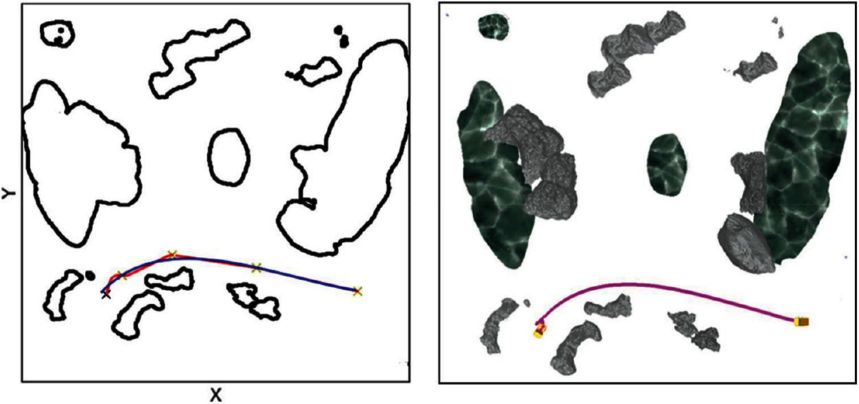
Figure 11: The path diagram for the second case

In the third case, the starting point is the bottom right corner and the end point is the top left corner. The verification results are shown in Fig. 12.

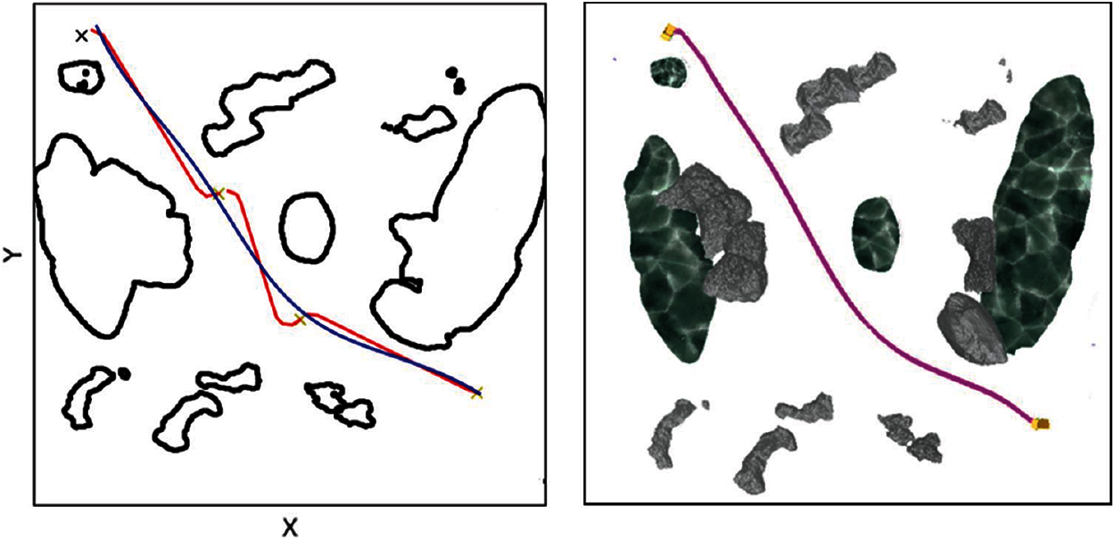
Figure 12: The path diagram for the third case

Finally, the parking attitude of the truck is adjusted based on the Reeds-sheep algorithm. As shown in Fig. 13, the white vehicle is the target attitude, the yellow vehicle is the starting state, and the pink line segment is the track line of the vehicle. From the final vehicle position and attitude, the error is almost zero, which proves that the control method mentioned above and the error correction in straight line driving are effective.

Figure 13: Parking attitude adjustment (a) go ahead and turn right (b) reverse to the left rear (c) reverse to the right rear (d) drive to the left front to reach the target position

4  Conclusion

In this paper, an improved bidirectional RRT* algorithm is proposed, which is applied to the path planning of mining trucks. Compared with the basic RRT* algorithm, the algorithm used in this paper mainly uses bidirectional RRT* and optimizes the path solving process of RRT*. These optimizations solve the problems of poor convergence, lack of stability and lack of guidance in the basic RRT algorithm. Finally, the path tracking based on Stanley algorithm is implemented by simulating a truck through simulation experiments in CoppeliaSim software, and the final results prove the correctness of the proposed method.

In the perspective of the future development of intelligent vehicles, even the improved bidirectional RRT* is based on model-driven, which will have limitations in practical application and cannot fully control the dynamic changes of vehicles. At present and for a long time to come, the direction of development should depend on algorithms such as RRT to react to dynamic situations in a timely manner through real-time data computation and local path planning.

Acknowledgement: This work was supported by the Suzhou Key industrial technology innovation project SYG202031.

Funding Statement: Suzhou Key industrial technology innovation project SYG202031.

Conflicts of Interest: The authors declare that they have no conflicts of interest to report regarding the present study.

This work is licensed under a Creative Commons Attribution 4.0 International License, which permits unrestricted use, distribution, and reproduction in any medium, provided the original work is properly cited.