DOI:10.32604/cmc.2022.022325
| Computers, Materials & Continua DOI:10.32604/cmc.2022.022325 | |
| Article |
Algorithm Development of Cloud Removal from Solar Images Based on Pix2Pix Network
1School of Information Engineering, Minzu University of China, Beijing, 100081, China
2Key Laboratory of Solar Activity, Chinese Academy of Sciences (KLSA, CAS), Beijing, 100101, China
3National Language Resource Monitoring and Research Center of Minority Languages, Minzu University of China, Beijing, 100081, China
4National Astronomical Observatories, Chinese Academy of Sciences (NAOC, CAS), Beijing, 100101, China
5Center for Solar-Terrestrial Research, New Jersey Institute of Technology, University Heights, Newark, 07102-1982, USA
6Institute for Space Weather Sciences, New Jersey Institute of Technology, University Heights, Newark, 07102-1982, USA
7Big Bear Solar Observatory, New Jersey Institute of Technology, 40386, North Shore Lane, Big Bear City, 92314-9672, USA
*Corresponding Author: Wei Song. Email: songwei@muc.edu.cn
Received: 04 August 2021; Accepted: 11 October 2021
Abstract: Sky clouds affect solar observations significantly. Their shadows obscure the details of solar features in observed images. Cloud-covered solar images are difficult to be used for further research without pre-processing. In this paper, the solar image cloud removing problem is converted to an image-to-image translation problem, with a used algorithm of the Pixel to Pixel Network (Pix2Pix), which generates a cloudless solar image without relying on the physical scattering model. Pix2Pix is consists of a generator and a discriminator. The generator is a well-designed U-Net. The discriminator uses PatchGAN structure to improve the details of the generated solar image, which guides the generator to create a pseudo realistic solar image. The image generation model and the training process are optimized, and the generator is jointly trained with the discriminator. So the generation model which can stably generate cloudless solar image is obtained. Extensive experiment results on Huairou Solar Observing Station, National Astronomical Observatories, and Chinese Academy of Sciences (HSOS, NAOC and CAS) datasets show that Pix2Pix is superior to the traditional methods based on physical prior knowledge in peak signal-to-noise ratio, structural similarity, perceptual index, and subjective visual effect. The result of the PSNR, SSIM and PI are 27.2121 dB, 0.8601 and 3.3341.
Keywords: Pix2Pix; solar image; cloud removal
The key to the research of the field of solar physics is to study the solar image to understand the structure and evolution of solar activity. Since the 1960s, observatories around the world have accumulated a large number of solar image data by monitoring solar activity. However, researchers are facing many difficulties in analyzing these images. Many of the observed images are obscured by clouds. For example, at the Big Bear Solar Observatory (BBSO) in California, USA, and the days that the observations were affected by clouds (may be from just a few images to large portion of the images during the day) occupy 55% of total days based on the site survey of the Global Oscillation Network Group (GONG) [1]. At other Observatories in the world, the percentage may be higher. In these days, instruments work normally; however, if cloud cover the Sun, their shadows will degrade the observed images. Therefore, it is of great significance for all ground-based observation stations to remove the contamination of cloud on the full-disk solar images [2]. Removing the effects of the clouds from the affected solar images becomes an urgent problem. As a key station in the world, the Halpha images of the solar chromosphere taken by Huairou Solar Observing Station (HSOS) provide ideal information for the detailed study of the subtle structure of the sun. There are some cloud-covered full disk images and normal full-disk images, which were observed by the HSOS (Fig. 1). Therefore, the research object is combined with the deep learning method, and use Pixel to Pixel network to get more cloudless full-disk Halpha images from the cloud-covered full-disk Halpha images.
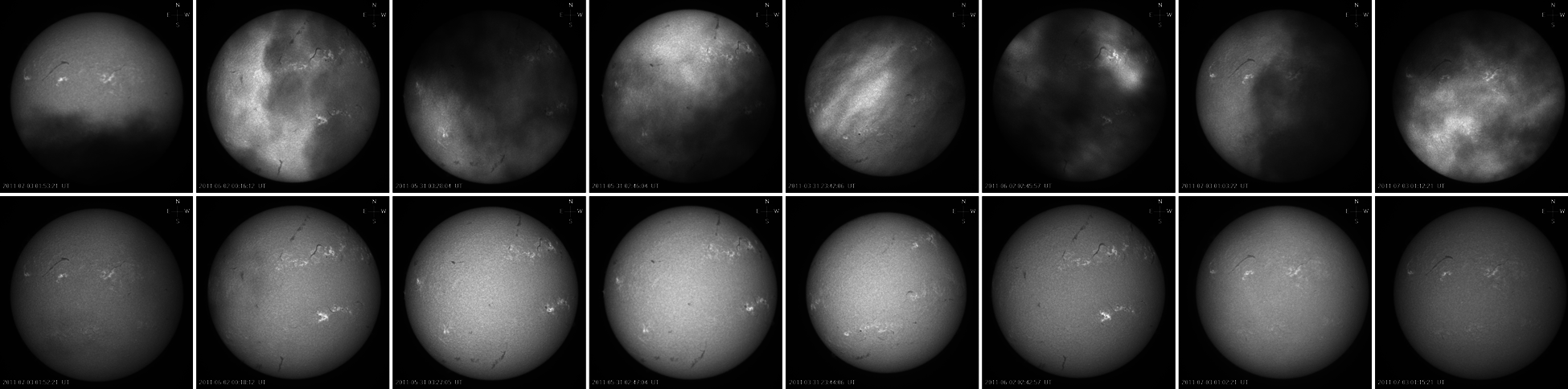
Figure 1: The top shows cloud-covered full-disk images and the bottom shows cloudless full-disk images, which were observed by the Huairou Solar Observing Station (HSOS) in 2011
The contributions of our work are as follows:
New method on cloud removal. Pix2Pix [3] is used for image cloud removal, which does not rely on the physical scattering model, while adopts the alternative image-to-image translation proposed in 2017.
U-Net Generator. Inspired by the global-first property of visual perception, the embedded U-Net Generator are designed to produce images with more details.
A joint training scheme. A joint training scheme is developed for updating the U-Net Generator through reasonably combining two kinds of loss functions.
The Perceptual Index (PI). PI is introduced for quantitative evaluation from the perceptual perspective. In addition, extensive experiments on solar dataset indicate that Pix2Pix performs favorably against the state-of-the-art methods. Especially, results are outstanding in visual perception.
The rest of the paper is structured as: Section 2 discusses the relevant work of processing solar images by traditional method and deep learning. Section 3 explains the image generation algorithm based on the Pix2Pix network, describes the process steps of the overall framework of the algorithm. Section 3 also gives the network structure diagram and loss function. Section 4 first explains how to generate training set and test set, and then compares and analyzes the effects of different modules in the algorithm presented on model performance. Finally, a large number of comparative experiments are carried out to analyze and evaluate the effectiveness of the proposed algorithm. The evaluation mainly starts from two aspects: subjective visual effect and objective evaluation index. Finally, the conclusion of the article will be presented.
2.1 The Traditional Method–DCP
Early cloud removal methods are mostly prior-based methods, and they can achieve a good cloud removal effect to a certain extent. Dark channel prior (DCP [4]) method, which estimates the transmission map by investigating the dark channel prior. Hu [5] propose a two-stage haze and thin cloud removal method based on homomorphic filtering and sphere model improved dark channel prior. Xu [6] propose a fast haze removal algorithm based on fast bilateral filtering combined with dark colors prior. Xu [7] propose a method based on signal transmission and spectral mixture analysis for pixel correction. HoanN [8] propose a cloud removal of remote sensing algorithm image based on multi-output support vector regression. Most of these approaches depend on the physical scattering model [9], which is formulated as Eqs. (1):
where I is the observed hazy image, J is the scene radiance, t is the transmission map, A is the atmospheric light and z is the pixel location. The solution of the cloudless image depends on the estimation of the atmospheric light and the transmission map.
DCP method on Fig. 2a produces a cloudless image with rich details compared with DCP method used on Fig. 2c. Therefore, the prior may be easily violated in practice, which leads to an inaccurate estimation of transmission map so that the quality of the cloud removal image is not desirable.
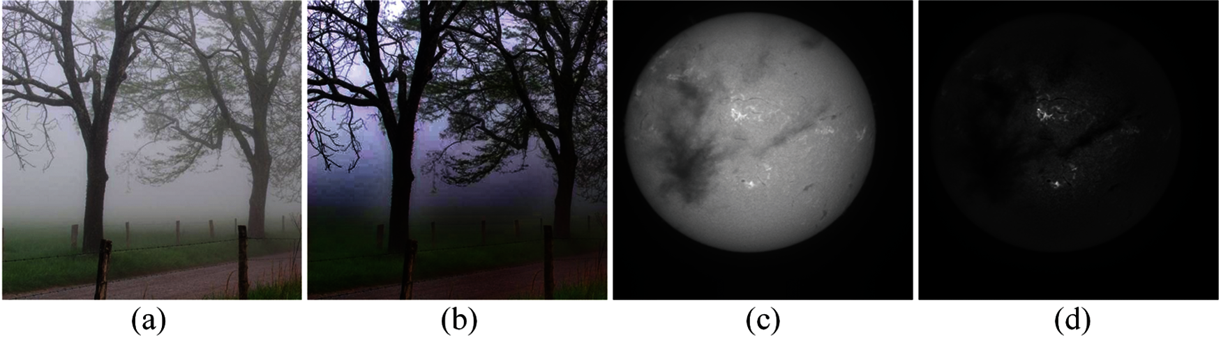
Figure 2: Examples of DCP method used on different images. (a) is the forest image affected by the cloud. (c) is the full disk solar image similarly affected. (b) and (d) are DCP processed images respectively
2.2 Deep Learning-Generative Adversarial Network
In recent years, researchers in the field of solar physics have gradually begun to explore the use of deep learning [10] to analyze and process solar activity observation data. The study of GAN [11] has made great progress. GAN is widely used in computer vision. In particular, GAN has achieved good results in image generation.
Densely Connected Pyramid Dehazing Network (DCPDN) [12] implements GAN on image cloud removal which learns transmission map and atmospheric light simultaneously in the generators by optimizing the final image cloud removal performance for cloudless images. Zhang et al. [13] proposed a real-time image processing system for detecting and removing cloud shadows on Halpha full-disk solar. Luo [14] identified that heavy cloud covered images by calculating the ratio of major and minor axes of a fitted ellipse. Sun [15] proposed the Cloud-Aware Generative Network. The network consists of two stages: the first is a recurrent convolution network for potential cloud region detection and the second is an auto encoder for cloud removal. Yang [16] proposed the disentangled cloud removal network, which uses unpaired supervision. The network proposed by Yang [16] contains three generators: the generator for the cloudless image, the generator for the atmospheric light, and the generator for transmission map. Zi [17] proposed a method to remove thin cloud from multispectral images, which combines the traditional method with the deep learning method. Firstly, Convolution Neural Network is used to estimate the thickness of thin cloud in different bands. Then, according to the traditional thin cloud imaging model, the thin cloud thickness image is subtracted from the cloud image to get a clear cloud image. DehazeGAN [18] draws lessons from the differential programming to draw lessons from GAN for simultaneous estimations of the atmospheric light and the transmission map. The use of GAN in image cloud removal task is still in the beginning. The current cloud removal methods via GAN all depend on the physical scattering model. Through the research on the development of GAN, it shows that CycleGAN realizes the transformation of unmatched data image. The image training set does not need paired data, so it is widely used. But the training set does not match, it can't be trained in absolute mapping relationship, only the real mapping relationship can be predicted. Therefore, the mapping relationship learned will deviate, which leads to unexpected transformation style of training results. The non-matching data is the input of two groups of completely unrelated data, which can achieve random image style conversion.
Until now, few papers discuss how to deal with image cloud removal independent of the physical scattering model. As discussed in Introduction, it is meaningful to investigate a model-free cloud removal method via GAN.
3 Cloud Removal Method Based on Pix2Pix
GAN is an unsupervised learning, it can't realize the conversion between pixels. Some researchers propose to use Conditional Generation Adversarial Network to complete the work of image to image, which is called Pix2Pix. It realizes the transformation of matching data image.
Pix2Pix Network adopts a fully supervised method (Fig. 3) that is to train the model with fully matched input and output images, and generate the target image of the specified task from the input image through the trained model. The algorithm is mainly divided into two stages: training and testing. In the training phase, the Pix2Pix network is trained with paired solar images, and then the network model is optimized by iterating the generation network and decision network to optimize the network parameters. In the test phase, the cloud-covered image is input into the trained Pix2Pix network to get the cloudless image.
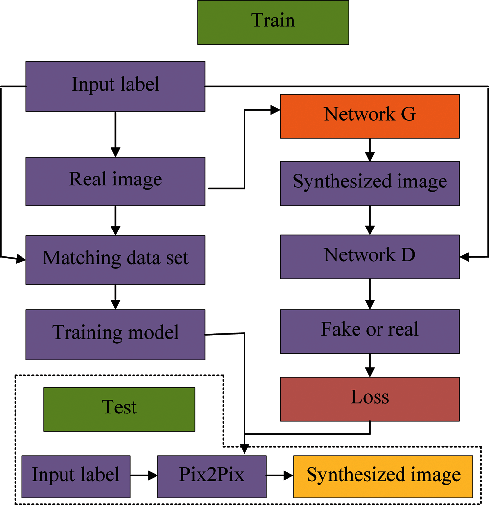
Figure 3: The flow chart of network
The generator adopts the U-Net [19] architecture (Fig. 4a). Eight convolution layers and eight deconvolution layers are used to generate pseudo samples. In the design of the discriminator (Fig. 4b), the network structure of 5 convolution layers and leaky relu layer is adopted. In generator G, the training Halpha images is input, and convolution operation is performed through 8 convolution layers. The activation function used in this part is leaky relu function, and the batch normalization method [20] is used in each layer to enhance the convergence performance of the model.
An 8-level U-Net architecture is employed for pixel-level feature learning. The architecture comprises of three parts: encoding network, decoding network, and a bridge that connects both the networks (Tab. 1). The complete network is constructed using 4 × 4 convolution layers with a stride of 2 for down-sampling and up-sampling.
U-Net architecture is used as Generator. U-Net architecture consists of two paths: a contractive path and an expansive path and both are symmetric to each other. It yields an architecture like U-shape (Fig. 5) (Thus called as U-Net). The network on the left side is a contracting path that is like a traditional CNN involving convolution and activations. On the right side of Fig. 5 is an expansive path which includes up-sampling layers and the corresponding convolutional layers on the left side. Both the network paths are merged to compensate for the loss of information. As a result, the architecture preserves the same resolution of images as in input network layer.
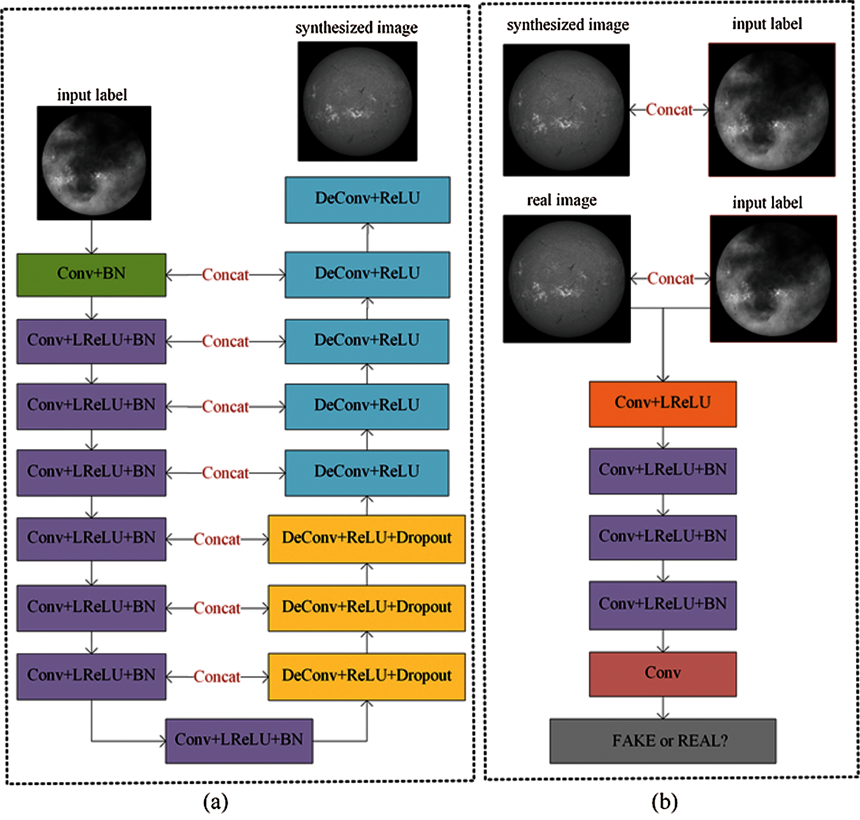
Figure 4: The architecture of Pix2Pix. Pix2Pix includes two parts: the U-Net generator and the Patch GAN discriminator. (a) Generator (b) Discriminator
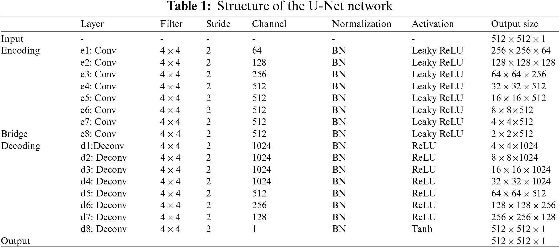
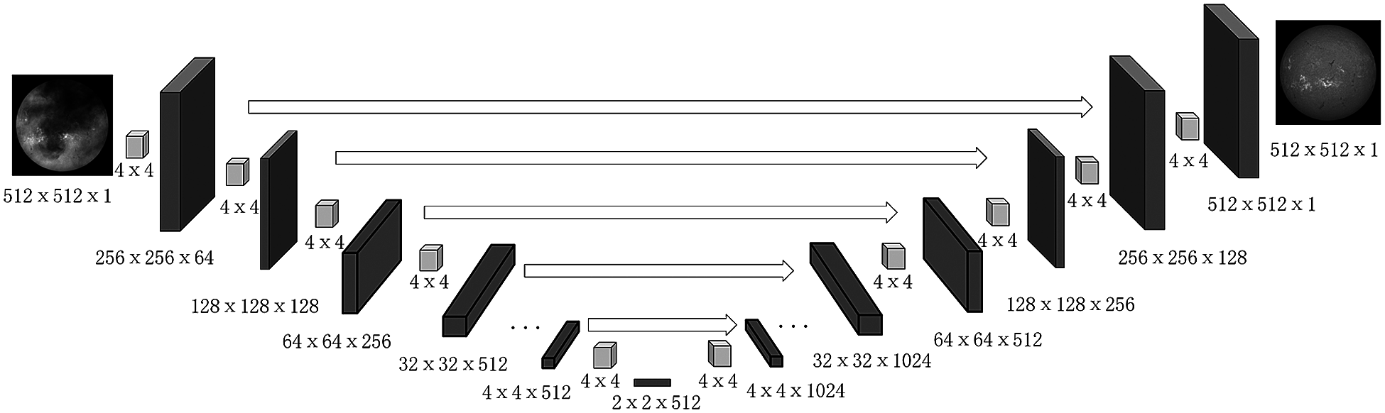
Figure 5: The structure of Generator
The discriminator uses PatchGAN (Fig. 6). PatchGAN makes the model more efficient and the detail achieves a better effect. The discriminator splices the image generated by the generator with the condition image. The number of convolution kernels in the first down-sampling layer is set to 64. The number of convolution kernels in each layer is set to twice that of the upper layer. The number of convolution kernels in the last down-sampling layer is set to 1. The first three down-sampling layers have a stride size of 2. The length and width of each image are half of the origin. The last two subsampling layers have a stride size of 1, keeping the image size unchanged. Finally, the results are obtained through the Sigmoid layer (Fig. 4).
The deeper the subsampling convolution layer is, the more accurate the extracted features will be. The size of the input image is 512 × 512, and each time the image is subsampled, the length and width of the image are changed to half of the original image. The feature image extracted from each layer of convolution is used as the criterion for discriminator. The size of feature image is the result of pixel, full image and patch. Fig. 7 indicated that the experimental results based on the patch were the best. So the PatchGAN is selected to be the discriminator.
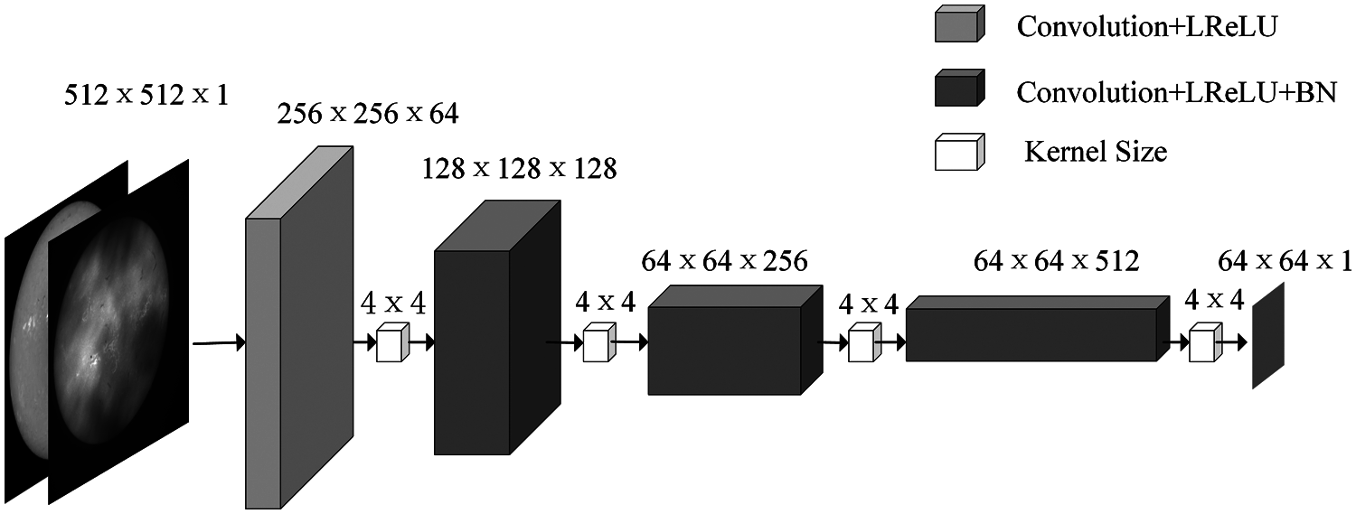
Figure 6: The structure of Discriminator
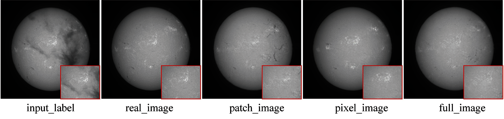
Figure 7: PatchGAN. The size of feature image is the result of pixel, full image and patch
The following is the loss function of Pix2Pix Network (Eqs. (2)). Where D(x, y) represents the result of the input object x and output object y of the real matching data for the discriminator D, while D(x, G (x, z)) is the result of the image G(x,z) generated by the generator for the discriminator. LCGAN(G, D) represents the loss function of CGAN. E represents the expectation.
In addition to the above-mentioned optimization function, Pix2Pix optimizes the network by adding LossL1[21] as the traditional loss function (Eqs. (3)).
The loss function of the final generator is shown in Eqs. (4), where λ is a hyperparameter, which can be adjusted as appropriate. When λ= 0, the loss function of LossL1is not used:
In this section, the data set is constructed to demonstrate the effectiveness of the proposed method. And four methods: Dark channel prior network (DCP), CGAN (Pix2Pix model without LossL1), L1 model (Pix2Pix model without LossGAN), CycleGAN are compared with the proposed method.
The data set is constructed which are partly provided by HSOS. The data set includes two parts: the full-disk Halpha solar images obscured by cloud and the cloudless full-disk Halpha solar images.82 typical pairs of Halpha images are selected as original training set, and 15 pairs of them are chosen to test the performance of the proposed method. Data augmentation is also critical for network in variance and robustness when a small number of training images are available. Flipping, shearing, zooming, and rotation are the main methods (Tab. 2). In order to obtain a usable model, only those images with distinct features are selected as training samples. Finally, 2731 samples are generated from 97 high-quality Halpha full-disk solar images. The proposed method takes 2566 pairs as inputs that are resized to 512 × 512 and sent to the enhanced Pix2Pix architecture to generate an appropriate weight model, which is used to removing cloud in Halpha images.

To better evaluate the performance of the proposed method, three image quality evaluation methods: the Peak Signal to Noise Ratio (PSNR) [22], the Structural Similarity (SSIM) [22] and Perceptual Index (PI) [23] can be used as image quality evaluation metrics.
Peak Signal to Noise Ratio (PSNR). The PSNR is a full-reference image quality evaluation indicator. Let MSE denote the mean square error between the current image X and the reference image Y; let H and W denote the image height and width, respectively. i and j represents the position of the pixel. Let n denote the number of bits per pixel (generally 8), meaning that the number of possible gray levels of a pixel is 256. The PSNR is expressed in units of dB. The larger the PSNR is, the smaller the distortion. The MSE (Eqs. (5)) and PSNR (Eqs. (6)) are calculated as follows:
Structural Similarity (SSIM). The SSIM is another full-reference image quality evaluation metric that measures image similarity from three perspectives: brightness, contrast, and structure. SSIM values closer to 1 indicate greater similarity between the original X and reconstructed image blocks Y and represent a better reconstruction effect. The formula for calculating the SSIM (Eqs. (7)) is as follows:
where, μxand μy represent the means of image blocks X and Y, respectively; σx, σyand σxy represent the variances of image blocks X, Y and their covariance, respectively; C1and C2 are constants.
Perceptual Index (PI). The PSNR and SSIM are the most commonly used objective indicators for image evaluation. PSNR is based on the error between corresponding pixels, which is based on error-sensitive image quality evaluation. SSIM is a full reference image quality evaluation index, which measures image similarity from brightness, contrast and structure. Since these measures do not consider the visual characteristics of the human eye, the evaluation results are often inconsistent with human subjective perception. PI (Eqs. (8)) is a new criterion which bridges the visual effect with computable index. And it has been recognized to be effective in image super-resolution [24] .In the experiment, PI is used to evaluate the performance of image cloud removal. The higher the image quality is, the lower PI is.
where, Ma and NIQE are two image qualification indexes which are detailed in [25].
4.3.1 The Number of Iterations
The loss value is recorded every 1000 iterations (Fig. 8). It can be seen from the change trend that the local minimum is reached around 1000,000 times, and then the discriminator continues to be trained to make the judgment more accurate. After 1000,000 times, the generated image is basically close to the target image and it tends to be stable, so the network trained by 1026,400 iterations is selected.
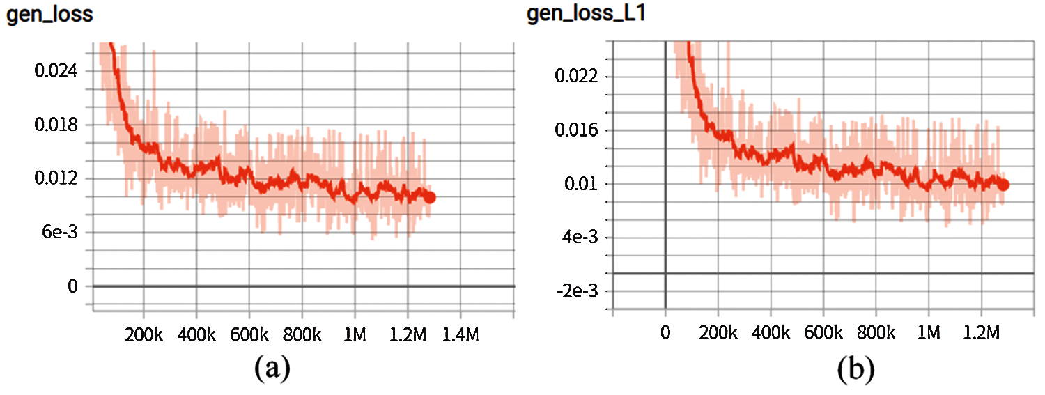
Figure 8: (a) is the change curve of LossGAN; values. The abscissa is the number of iterations and the ordinate is the value of the Generator loss function. (b) is the change curve of LossL1 values. The abscissa is the number of iterations and the ordinate is the value of the LossL1 function
The adjustment of this parameter is mainly to consider the weight of the two loss functions. It aims to make the detail information of the generated image closer to the real image. That is, make the generator more accurate. So consider taking λ to 100 and 0 respectively. When λ = 0, the loss function only has LossGANand it doesn't has LossL1Block effect will appear when loss function is defined as LossGAN, block uniform stripes will appear in the image, causing image distortion (Fig. 9). When loss function is defined as Loss=LossGAN+LossL1 block effect of the image is significantly weakened or even disappeared, which improves the texture clarity of the image. In the experimental comparison of parameter sizes, LossGANand LossL1are not on the same order of magnitude, and the influence of LossL1 should be appropriately increased without affecting the function of LossGAN(Fig. 8). Therefore, the weight is increased to make the generated image closer to the target image.
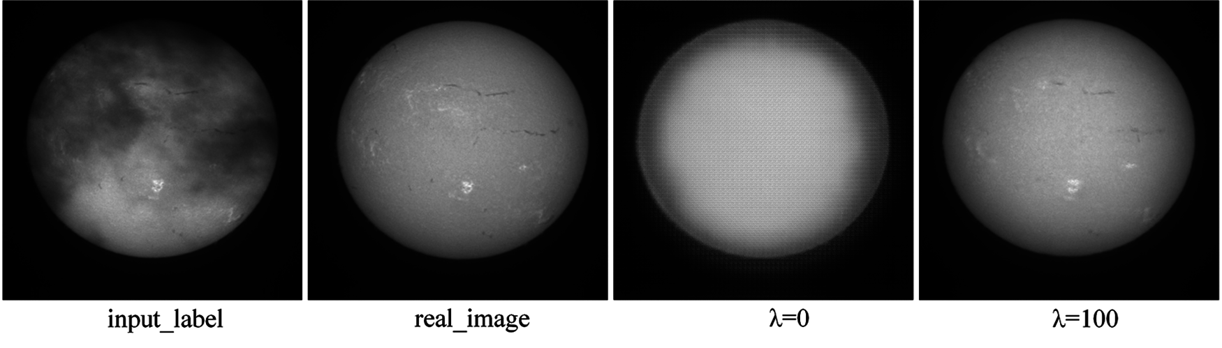
Figure 9: The experimental results of different loss functions, When λ= 0, the loss function only has LossGAN and no LossL1. When λ=100, the loss function has LossGAN and LossL1
1, 10, 30, 50, 70, 90, 100 were set as the value of λ respectively (Tab. 3).Subjective comparison was conducted under the results of 1,026,400 iterations. As the value of λ increases, the PSNR and SSIM significantly increases. And the overall perceived quality is better. The PSNR is 27.2121, which is 0.5 dB higher than other results, the SSIM is 0.8601, which is also higher than other results. The experimental results show that as the value of λ increases, the PI significantly decreases (Fig. 10). Therefore, from the three image quality evaluation methods, the choice of 100 as the value of λ is the best.

The method is performed on the tensorflow framework and a NVIDIA GeForce RTX2080ti GPU. During training, Adam optimizer [26] is adopted with a batch size of 1, and set a learning rate as 0.0002. The hyperparameters of loss function is set as λ = 100. The discriminator tended to converge after about 1,026,400 iterations on the training set. Fig. 11 shows the results of test set in 2011. From left to right are the cloud covered Halpha images, the generated cloudless images and the real cloudless images. It can be seen that the model has a good generating effect on the test set. Dark thread-like features are filaments and bright patches surrounding sunspots are plages which are also associated with concentrations of magnetic fields. So the characteristic areas on the figure are restored and the cloud is removed.
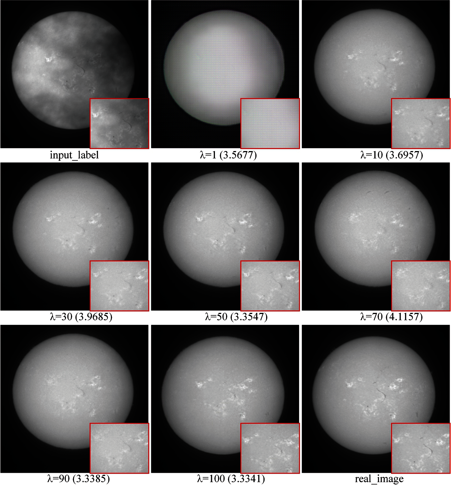
Figure 10: Experimental results with different λ values, PIs are shown at the bottom of each image
4.5 Comparisons with Other Methods
Fig. 12 gives the comparison of visual effect in which the comparison results on proposed data set. DCP method suffers from color distortion, where the results are usually darker than the ground truth images and it is observed that there remains some cloud in the images. CGAN suffers from color distortion and it fails in details restoration. In the L1 loss model, the generated picture also loses detail information, and there is noise in the generated picture. Compared with CycleGAN, Pix2Pix makes the synthesized image look more like the ground truth image. It is obvious that Pix2Pix out-performs the above mentioned methods in details recovery, and it improves the cloud removal results qualitatively and quantitatively.
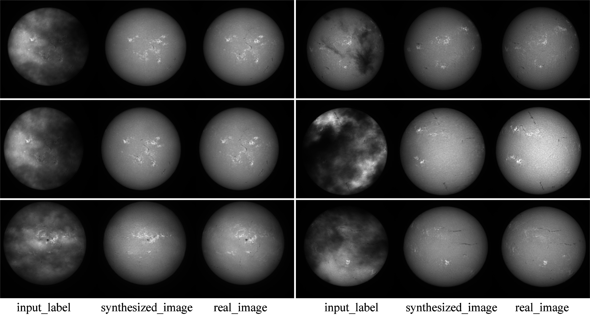
Figure 11: The experimental results of the Pix2Pix model test
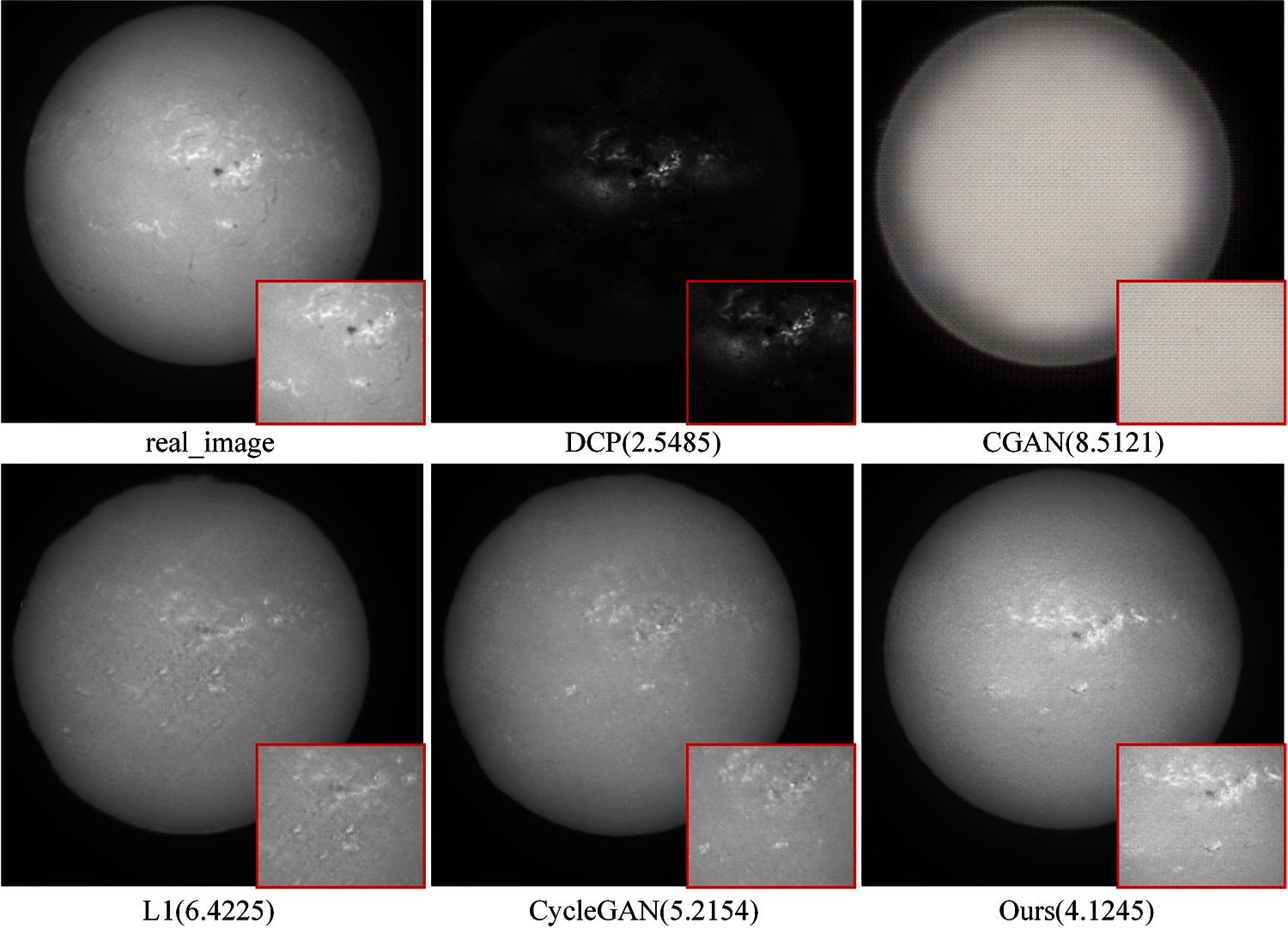
Figure 12: Results of comparison between DCP, CGAN, L1 model, CycleGAN and the proposed method. PIs are shown at the bottom of each image
The SSIM value obtained by Pix2Pix is 0.8601, and the PSNR value is 27.2121 dB (Tab. 4). Both of them are higher than other four models. From these two indicators, the cloud removal effect of Pix2Pix model is better than other models, which is consistent with the subjective perception of the target image. According to the description of PI index, the lower the PI value, the higher the image quality. The PI value of the DCP model is the smallest (Fig. 12). The image has been sharpened after DCP processing, but the goal of image cloud removal has not been achieved. After excluding the DCP model, the Pix2Pix model performs the best. From these three objective indicators, it can indirectly prove that the algorithm in this paper can better generate the details and features of the image, make the generated image closer to the real image and remove the influence of cloud on the full disk data set of solar image. The achieved results conclude the proposed model as an effective model among all the used models in this investigation.

The proposed method is not very robust for heavily cloud scene (Fig. 13), the details of solar image in heavily cloud can't be recovered naturally. The size of data set is not big enough and core details of images can't be learned. The limitation might be solved by applying enhancing blocks in the network.
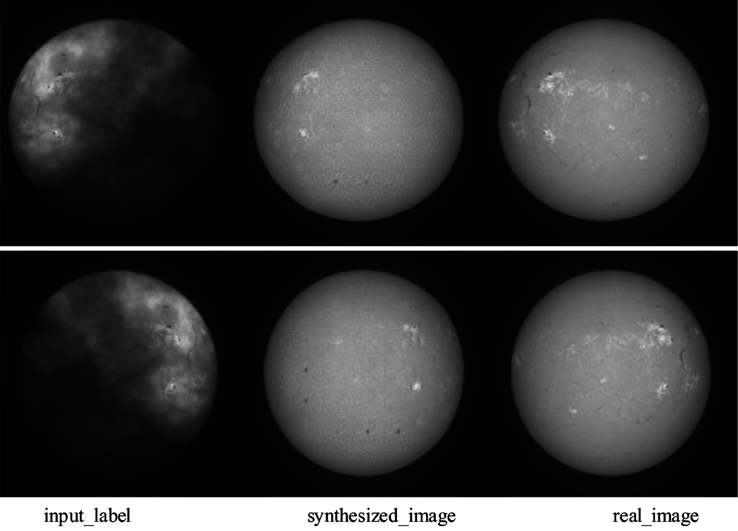
Figure 13: An example for heavily cloud scene
Imaging analysis and processing are critical components in solar physics. It is difficult for researchers to analyze solar activity in images obscured by clouds. Therefore, it is of great significance to remove the cloud from the image for all ground-based observations. This paper uses an image translation algorithm based on pixel to pixel network for image cloud removal. In this network, a U-Net generator and PatchGAN discriminator is used to improve the generated image details, so that the visual effect of the generated cloudless image is more realistic, and the goal of image cloud removal is realized. And it is compared with the traditional mainstream deep learning image generation algorithms. In these experiments, it be found that the model can learn more effective solar image features and synthesize clearer cloudless images by using the data set of the National Astronomical Observatories. The results of this study will be deployed to HSOS to improve the image quality of the full disk data set of solar image. The proposed method will also use image processor technology to develop corresponding processing software for astronomical observation researchers. The future work will focus on creating a larger data set from solar images, obtaining a data set with various solar activity conditions, making the network have better generalization capabilities, and studying some different quantitative performance indicators to evaluate our method.
Acknowledgement: Authors are thankful to the Huairou Solar Observing Station (HSOS) which provided the data. Authors gratefully acknowledge technical and financial support from CAS Key Laboratory of Solar Activity, Media Computing Lab of Minzu University of China and New Jersey Institute of Technology. We acknowledge for the data resources from “National Space Science Data Center, National Science Technology Infrastructure of China. (https://www.nssdc.ac.cn).
Funding Statement: Funding for this study was received from the open project of CAS Key Laboratory of Solar Activity (Grant No: KLSA202114) and the crossdiscipline research project of Minzu University of China (2020MDJC08).
Conflicts of Interest: The authors declare that they have no conflicts of interest to report regarding the present study.
1. F. Hill, G. Fischer, S. Forgach, J. Grier, J. W. Leibacher et al., “The global oscillation network group site survey,” Solar Physics, vol. 152, pp. 321–349, 1994. [Google Scholar]
2. S. Feng, J. Lin, Y. Yang, H. Zhu, F. Wang et al., “Automated detecting and removing cloud shadows in full-disk solar images,” New Astronomy, vol. 32, pp. 24–30, 2014. [Google Scholar]
3. P. Isola, J. Zhu, T. Zhou and A. Efros, “Image-to-image translation with conditional adversarial networks,” in 2017 IEEE Conf. on Computer Vision and Pattern Recognition, Hawaii, USA, vol. 12, pp. 5967–5976, 2017. [Google Scholar]
4. K. He, J. Sun and X. Tang, “Single image haze removal using dark channel prior,” in 2009 IEEE Conf. on Computer Vision and Pattern Recognition, Miami, Florida, USA, vol. 32, pp. 1956–1963, 2009. [Google Scholar]
5. G. Hu, X. Sun, D. Liang and Y. Sun, “Cloud removal of remote sensing image based on multi-output support vector regression,” Journal of Systems Engineering and Electronics, vol. 25, pp. 1082–1088, 2014. [Google Scholar]
6. H. Xu, J. Guo and Q. Liu, “Fast image dehazing using improved dark channel prior,” in 2012 IEEE Int. Conf. on Information Science and Technology, Wuhan, China, vol. 128, pp. 663–667, 2012. [Google Scholar]
7. M. Xu, A. J. Plaza and X. Jia, “Thin cloud removal based on signal transmission principles and spectral mixture analysis,” IEEE Transactions on Geoscience and Remote Sensing, vol. 54, no. 3, pp. 1659–1669, 2016. [Google Scholar]
8. T. HoanN and R. Tateishi, “Cloud removal of optical image using SAR data for ALOS applications experimenting on simulated ALOS data,” Journal of the Remote Sensing Society of Japan, vol. 29, no. 2, pp. 410–417, 2009. [Google Scholar]
9. E. M. Cartney and F. Hall, “Optics of the atmosphere: Scattering by molecules and particles,” Physics Today, vol. 30, no. 5, pp. 76, 1976. [Google Scholar]
10. L. Z. Tao, L. W. Lin, L. F. Yuan, S. Yi, Y. Min et al., “Hybrid malware detection approach with feedback-directed machine learning,” Science China Information Sciences, vol. 22, pp. 139–103, 2020. [Google Scholar]
11. J. P. Abadie, M. Mirza, B. Xu and D. Farley, “Generative adversarial networks,” Communications of the ACM, vol. 63, no. 11, pp pp. 139–144, 2014. [Google Scholar]
12. H. Zhang and V. M. Patel, “Densely connected pyramid dehazing network,” in 2018 IEEE Conf. on Computer Vision and Pattern Recognition, Salt Lake City, USA, vol. 22, pp. 3194–3203, 2018. [Google Scholar]
13. N. Zhang, Y. Yang, R. Li and K. Ji, “A real-time image processing system for detecting and removing cloud shadows on halpha full-disk solar,” (In ChineseAstronomical Research and Technology, vol. 13, no. 2, pp, pp. 242–249, 2016. [Google Scholar]
14. L. Luo, Y. Yang, K. Ji and H. Deng, “Halpha algorithm based on edge dim contour alpha quality evaluation of full solar image,” (In ChineseActa Astronomica Sinica, vol. 54, pp. 90–98, 2004. [Google Scholar]
15. L. Sun, Y. Zhang, X. Chang and J. Xu, “Cloud-aware generative network: Removing cloud from optical remote sensing images,” IEEE Geoscience and Remote Sensing Letters, vol. 17, no. 4, pp. 691–695, 2020. [Google Scholar]
16. X. Yang, X. Zheng and J. Luo, “Towards perceptual image dehazing by physics-based disentanglement and adversarial training,” in Proc. of the AAAI Conf. on Artificial Intelligence, New Orleans, Lousiana,USA, vol. 32, no. 1, 2018. [Google Scholar]
17. Y. Zi, F. Xie, N. Zhang, Z. Jiang, W. Zhu et al., “Thin cloud removal for multispectral remote sensing images using convolutional neural networks combined with an imaging model,” IEEE Journal of Selected Topics in Applied Earth Observations and Remote Sensing, vol. 14, pp. 3811–3823, 2021. [Google Scholar]
18. H. Zhu, X. Peng, L. Li and L. J. Hwee, “DehazeGAN: when image dehazing meets differential programming,” in Proc. of the Twenty-Seventh Int. Joint Conf. on Artificial Intelligence, Stockholm,Sweden, vol. 33, pp. 1234–1240, 2018. [Google Scholar]
19. H. Li, C. Pan, Z. Chen, A. Wulamu and A. Yang, “Ore image segmentation method based on u-net and watershed,” Computers, Materials & Continua, vol. 65, no. 1, pp. 563–578, 2020. [Google Scholar]
20. S. Ioffe and C. Szegedy, “Batch normalization: Accelerating deep network training by reducing internal covariate shift,” in the 32nd Int. Conf. on Machine Learning, Lille, France, vol. 37, pp. 448–456, 2020. [Google Scholar]
21. X. Fu, L. Wei, L. Z. Tao, C. L. Chen and W. R. Chuan. “Noise-tolerant wireless sensor networks localization via multi-norms regularized matrix completion,” IEEE Transactions on Vehicular Technology, vol. 64, pp. 2409–2419, 2018. [Google Scholar]
22. A. Horé and D. Ziou, “Image quality metrics: PSNR vs. SSIM,” in 2010 20th Int. Conf. on Pattern Recognition, Istanbul, Turkey, vol. 23, pp. 2366–2369, 2010. [Google Scholar]
23. Y. Blau, M. Zhao, X. Liu, X. Yao and K. He, “Better visual image super-resolution with laplacian pyramid of generative adversarial networks,” Computers, Materials & Continua, vol. 64, no. 3, pp. 1601–1614, 2020. [Google Scholar]
24. K. Fu, J. Peng, H. Zhang, X. Wang and F. Jiang, “Image super-resolution based on generative adversarial networks: A brief review,” Computers, Materials & Continua, vol. 64, no. 3, pp. 1977–1997, 2020. [Google Scholar]
25. A. Mittal and A. C. Bovik, “Making a completely blind image quality analyzer,” IEEE Signal Processing Letters, vol. 20, no. 3, pp. 209–212, 2013. [Google Scholar]
26. D. King and J. Ba, “Adam: A method for stochastic optimization, compute,” in 3rd Int. Conf. for Learning Representations, San Diego, CA, USA, vol. 26, pp. 14–17, 2015. [Google Scholar]
 | This work is licensed under a Creative Commons Attribution 4.0 International License, which permits unrestricted use, distribution, and reproduction in any medium, provided the original work is properly cited. |