DOI:10.32604/cmc.2022.022414
| Computers, Materials & Continua DOI:10.32604/cmc.2022.022414 | |
| Article |
Feature Selection for Cluster Analysis in Spectroscopy
1College of Engineering, IT & Environment, Charles Darwin University, Casuarina, NT 0909, Australia
2Defence Science and Technology Group, Edinburgh, 5111, Australia
3Energy and Resources Institute, Charles Darwin University, Casuarina, NT 0909, Australia
*Corresponding Author: Suresh N. Thennadil. Email: suresh.thennadil@cdu.edu.au
Received: 06 August 2021; Accepted: 07 September 2021
Abstract: Cluster analysis in spectroscopy presents some unique challenges due to the specific data characteristics in spectroscopy, namely, high dimensionality and small sample size. In order to improve cluster analysis outcomes, feature selection can be used to remove redundant or irrelevant features and reduce the dimensionality. However, for cluster analysis, this must be done in an unsupervised manner without the benefit of data labels. This paper presents a novel feature selection approach for cluster analysis, utilizing clusterability metrics to remove features that least contribute to a dataset's tendency to cluster. Two versions are presented and evaluated: The Hopkins clusterability filter which utilizes the Hopkins test for spatial randomness and the Dip clusterability filter which utilizes the Dip test for unimodality. These new techniques, along with a range of existing filter and wrapper feature selection techniques were evaluated on eleven real-world spectroscopy datasets using internal and external clustering indices. Our newly proposed Hopkins clusterability filter performed the best of the six filter techniques evaluated. However, it was observed that results varied greatly for different techniques depending on the specifics of the dataset and the number of features selected, with significant instability observed for most techniques at low numbers of features. It was identified that the genetic algorithm wrapper technique avoided this instability, performed consistently across all datasets and resulted in better results on average than utilizing the all the features in the spectra.
Keywords: Cluster analysis; spectroscopy; unsupervised learning; feature selection; wavenumber selection
1.1 Cluster Analysis in Spectroscopy
Cluster analysis is an unsupervised machine learning technique aimed at generating knowledge from unlabeled data [1]. While cluster analysis is a well-established domain, it is a highly subjective field with many potential techniques whose success will vary depending on the characteristics of the data and the purpose of the analysis. Clustering is very much a human construct, hence, mathematical definitions are challenging and even the definition of good clustering is subjective [2].
While cluster analysis is commonly used for data exploration, there are other circumstances where it is valuable such as when the class structure is known to vary with time, or the cost of acquiring classified (labeled) samples might be too great [3]. The latter is often the case for data from spectroscopic chemical analysis.
Spectroscopy is the study of interaction between matter (the material being analyzed) and electromagnetic radiation, as a function of the wavelength or frequency of the electromagnetic radiation. The transmission or absorption of the electromagnetic radiation through a given material varies by wavelength, producing a characteristic spectrum for that material. It is these resultant spectra that are the subject of our analysis. Examples of forms of spectroscopy include Fourier transform infrared (FTIR), UV-vis, mid infrared (Mid-IR), near infrared (NIR), and Raman spectroscopy. While the physical mechanisms for obtaining measurements differ between the various forms of spectroscopy, the general data characteristics are similar.
Spectroscopy data is typically of high dimensionality. A large number of measurements are taken at intervals across a spectrum for each sample. Depending on the type of spectroscopy and the specifics of the instrumentation, the number of features is typically in the hundreds or thousands for each sample. In other cluster analysis literature [4], 50 dimensions is referred to as high dimension data, yet spectroscopy data is typically significantly higher dimension than that. Hence, this high dimensionality needs special consideration in determining analytical approaches.
Spectroscopy data typically contains a relatively low number of samples or datapoints. Spectroscopy is usually used in laboratory or in process plants where collecting and processing samples can be an expensive process from the perspective of cost, time, and expertise. Hence, typically the number of samples is small, particularly from a machine learning perspective where big data has become a dominant focus.
These characteristics present unique challenges that focus and somewhat limit the techniques suitable for analysis of spectroscopy data and are a driver for the use of cluster analysis. Unsupervised learning techniques are well suited to chemical analysis applications where obtaining the large data sets and the associated labeling of data required for some supervised learning techniques is often infeasible [5].
Hence, this paper presents a novel perspective specific to the needs of cluster analysis in spectroscopy, namely, feature selection techniques to address the challenge of high dimensionality in spectroscopy data.
1.2 Feature Selection for Cluster Analysis in Spectroscopy
To improve the outcomes of cluster analysis in spectroscopy, data pre-processing and feature selection are often employed. Both work to improve the quality of data for cluster analysis by removing unwanted noise, anomalies, and irrelevant information to focus the cluster analysis on the information of interest within a dataset. While data pre-processing is important in improving clustering results, this is addressed elsewhere in literature from the chemometric community where effective techniques have been developed for pre-processing spectroscopy data. However, the literature and application examples for feature selection techniques for cluster analysis of spectroscopy is limited [6], hence why it is the focus of our paper.
Unsupervised feature selection can provide benefits through higher clustering accuracy, lower computational costs, and easier interpretability. Feature selection may also be referred to as feature mining, attribute selection, variable subset selection, variable reduction, wavelength selection, or wavenumber selection depending on the preferred terminology in a subject area.
This paper presents our novel feature selection approach, focused on applications for cluster analysis. Specifically, it is an unsupervised filter technique utilizing clusterability metrics to remove features that least contribute to a dataset's tendency to cluster. Two versions are presented and evaluated: The Hopkins clusterability filter which utilizes the Hopkins test for spatial randomness and the Dip clusterability filter which utilizes the Dip test for unimodality.
Associated with this is a wider evaluation of feature selection techniques for cluster analysis of spectroscopy data. While each of these aspects in isolation are widely addressed elsewhere, there has not been a combination of these specific focuses of research. Hence, this paper presents techniques and real-world evaluation results of value for researchers (such as chemometricians) looking to improve spectroscopy-based cluster analysis results through feature selection.
Finally, an evaluation and visualization technique is presented and utilized to provide confidence that the feature selection techniques will lead to improved clustering outcomes when applied to unlabeled datasets (as per the typical application of unsupervised learning).
Feature selection for cluster analysis in spectroscopy presents some unique challenges. For example, the nature of typical spectroscopy data (very high dimensionality, low sample size) preclude the application of many cutting-edge techniques where cluster analysis research is currently focused. E.g. cluster analysis with deep learning [7].
Similarly, the vast majority of the feature selection literature from the machine learning domain focuses on applications where targets (labels) exists. i.e., supervised learning. These supervised learning approaches to feature selection are not valid for the application of cluster analysis unless they can be adapted to work with unlabeled datasets. Much of the feature selection literature from the chemometric domain also focuses on applications of classification and regression and the associated calibration using well proven techniques such as partial least squares (PLS) and principal component regression (PCR) [8–10]. It has not been demonstrated if feature selection methods associated with these techniques are applicable for cluster analysis.
There is literature focused on feature selection for cluster analysis [11–16], and in recent years, unsupervised feature selection methods have raised considerable interest in many research areas. Recently, Solorio-Fernández, Carrasco-Ochoa, and Martínez-Trinidad presented a substantial review and evaluation of many unsupervised feature selection techniques [17]. However, these studies do not address the characteristics of spectroscopy data and either demonstrate techniques on relatively low dimensionality datasets [11,17], or are focused on domains such as social media data where large sample sizes are common [18]. This means some of these techniques are mis-matched for the small sample sizes that are typical in spectroscopy.
Given the lack of literature addressing our application for feature selection for cluster analysis of spectroscopy, we now consider the available techniques and their suitability. Feature selection techniques can generally be broken down into the categories of manual selection, filter methods, wrapper methods, hybrid methods and embedded methods.
Manual feature selection techniques, also referred to as knowledge based selection, utilize a priori knowledge of the subject material of interest and the testing method employed [8]. These methods are common in the chemical analysis domains, as employed by chemometricians. Examples of this include removing regions where instruments are known to be insensitive such as the higher and lower regions of the spectra, or regions where there is a low signal-to-noise ratio. Additionally, the expertise of analytical chemists may be utilized to select spectral peaks that enable differentiation of known chemical components. Drawbacks of these approaches include the requirement for subject matter expertise in the spectroscopy technique. Additionally, there is a potential for mismatch between the manual “human feature selection” process and the machine learning cluster analysis. The intrinsic non-linearity of spectroscopy and its relationship to the analytical parameters contribute to this [19]. Removal of information that appears non-optimal to the human may contain valuable information for the machine learning model [8]. These manual feature selection methods will not be addressed in this paper as our focus is on automated methods without the need for a priori knowledge or subject matter expertise.
Filter methods evaluate the relevance of a feature by studying its characteristics using certain statistical criteria. They are independent of the clustering algorithm and are typically fast to execute. In application, filter models are the most popular, especially for problems with large datasets [16]. While there are many filter methods available, most are focused on supervised learning where target values (labeled data) are available and used as part of the statistical criteria, most commonly assessing correlation between features and the class labels [20]. For unsupervised learning and cluster analysis, these labels are typically not available, hence a subset of techniques suitable for unsupervised learning are evaluated in this paper. There are also multiple techniques developed specifically for cluster analysis or unsupervised feature selection, as summarized in reviews by Alelyani et al. [16] and Solorio-Fernández et al. [17]. Later, we also present our novel filter method targeted at cluster analysis.
Wrapper methods of feature selection utilize a learning algorithm and the resulting outcomes as a selection criterion. For cluster analysis, this is the selected clustering algorithm. Since the full clustering algorithm is executed on the candidate feature sets, wrapper methods are typically computationally expensive [17]. Evaluating all possible subsets of features is near impossible in high-dimensional datasets. Therefore, a heuristic search strategy is adopted to reduce the search space. Wrapper method feature selection may be biased to the chosen ‘classifier’ (clustering algorithm) [16] and lack robustness across different cluster algorithms [15]. However, it is often the preferred method when accuracy is important [15].
Embedded methods performs feature selection as part of the learning or clustering algorithm itself [16]. We will not explore embedded methods in this paper as techniques evaluated are those that are applicable to multiple clustering algorithms.
Hybrid methods were proposed to bridge the gap between the filter and wrapper models. First, they use the statistical criteria of a filter method to select several candidate features subsets with a given cardinality. Then, apply the clustering algorithm and assessment metric to identify the subset which results in the highest clustering accuracy (as per a wrapper method). Thus, the hybrid model usually achieves both near comparable accuracy to the wrapper and near comparable efficiency to the filter model.
A selection of the above feature selection techniques will now be evaluated for our application in spectroscopy.
3.1 Datasets and Characteristics
As with most aspects of cluster analysis, a technique's success is often dependent on how well suited it is to the characteristics of specific datasets. Our specific research interest is in cluster analysis of homemade explosive samples, so feature selection techniques are evaluated against three datasets of homemade explosives. However, there is an interest in understanding how widely applicable these techniques are to other datasets. Hence, the techniques are also applied to cluster analysis of eight additional publicly available real-world spectroscopy datasets covering food chemistry, industrial production and biomedical domains.
The explosives samples used in this study are representative samples of homemade explosive detonators used in the Middle East in improvised explosive devices (IED). Detonators are a small explosive device used to detonate the larger bulk explosive main charge in an IED. The function of a detonator is to accept a command impulse (e.g., electrical current) and progressively amplify this into an explosive shock delivered to the larger main explosive charge. Detonators typically uses several different energetic materials in a sequence that imparts a different output as the shock wave passes along the device. The detonators used in this study consist of three stages of explosives of varying chemistries. This generates three data sets for comparison and are labeled: the First Fire Energetic, the Transition Energetic, and the Output Energetic. Fourier Transform Infrared (FTIR) spectroscopy data from each of the three stages of the detonators has been collected using an attenuated total reflectance (ATR) configuration. A scan of the sample is taken covering the infrared frequency range of 650–4000 cm−1. This results in 3350 measurements per sample (features) and the datasets consisted of 53, 69 and 73 explosive samples each.
To explore the wider applicability of feature selection techniques for clustering of spectroscopy data, additional publicly available spectroscopy datasets were analyzed. These include mid-infrared, near infrared (NIR), and Fourier transform infrared (FTIR) spectroscopy and are described as follows and summarized in Tab. 1:
• A collection of 56 mid infrared diffuse reflectance (MIR-DRIFT) spectroscopy spectra of lyophilized coffee produced from two species: arabica and canephora var. robusta [21].
• A collection of 983 FTIR spectroscopy spectra from different authenticated fruit purees in one of two classes: “Strawberry” and “Non-Strawberry” (strawberry adulterated with other fruits and sugar solutions) [22].
• A collection of 731 FTIR spectroscopy spectra from liver and annotated according to the majority presence of a chemical compound (collagen, glycogen, lipids, or DNA) in that part of the cell [23].
• A collection of 186 NIR spectroscopy spectra from intact mango fruits from 4 different cultivars [24].
• A collection of 32 FTIR spectroscopy spectra from nine marzipan types [25].
• A collection of 120 FTIR spectroscopy spectra from fresh minced meats–chicken, pork and turkey [26].
• A collection of 120 FTIR spectroscopy spectra from 60 different authenticated extra virgin olive oils from four geographic regions [27].
• A collection of 44 FTIR spectroscopy spectra (with the ‘water-band’ removed) from wine from four geographic regions [28].

Initial spectral data pre-processing can directly influence the outcomes when analyzing spectroscopy data [29]. Spectral pre-processing prior to cluster analysis can help in removing or reducing unwanted signals from data such as experimental and instrumental artefacts.
In our analysis, extended multiplicative signal correction (EMSC) [30] was selected for application to all spectroscopy datasets. EMSC includes corrections for constant offset, the gradient of the sloping baseline, interference effects, and a multiplicative scaling factor from reference signal and has regularly been demonstrated to give superior results to other pre-processing techniques for spectroscopy [31,32]. The EMSC was implemented for our analysis using Orange3 data mining toolbox in Python [33].
3.3 Cluster Analysis Algorithm Selection
For the cluster analysis conducted within our study, agglomerative hierarchical clustering was chosen as the hierarchical output aspect may be useful for identifying group or source attribution of bomb-makers from our homemade explosives datasets. Variants of hierarchical clustering algorithms are differentiated by the rules they use to form the links between datapoints and hence, the clusters. Examples include single link, complete link, average link and Ward's method [34]. Ward's method has been demonstrated as the most effective in several spectroscopy applications [35,36] and, hence, was selected for our analysis and Euclidean distance was used as the similarity measure for our cluster analysis of the spectroscopy data.
Predicting the number of clusters within a dataset is also a significant challenge for cluster analysis. However, that is not the focus of this study. Since labeled datasets are being used in the evaluation of the feature selection techniques, the number of clusters are known. This a priori knowledge is used to set the number of clusters for the hierarchical clustering. If this information was not available, techniques such as the “elbow” method [37], the gap statistic [37], and peak silhouette score [38] could be used for predicting the number of clusters.
3.4 Feature Selection Techniques: Filter Methods
The categories of filter methods and the specific feature selection techniques used in this paper are now presented, including our novel “clusterability filter” methods. While many more potential techniques exist within each category, this subset has been selected as representative examples of commonly applied techniques suitable for application to cluster analysis of spectroscopy (while limiting the study to a manageable size).
Filter methods for feature selection evaluate the relevance of a feature or a subset of features by studying its characteristics using statistical criteria. Since no data labels are available for this calculation, the independent statistical tests that we have utilized are as follows:
• Variance, which is one of the simplest metrics for evaluation of features [20].
• Dispersion, which is the arithmetic mean divided by the geometric mean. Higher dispersion may correspond to more relevant features.
• Mean Absolute Deviation, which is a robust measure of variability computed as the mean absolute deviation from the mean value.
These statistical measures are computed for each feature and the top ranked features are selected. It should be noted that although criteria such as the Variance find features that maximize representation of the dataset, these may not necessarily relate to clustering and being able to discriminate between data from different clusters. These are generic information-based filters, not specifically tuned for cluster analysis. They are low-complexity in nature making them fast and well suited for application to large datasets or as a precursor to computationally intensive operations. However, they are univariate in nature and do not consider possible correlation between different features [17].
Multi-Cluster Feature Selection (MCFS), developed by Cai et al. [14] has been selected as a representative of filter techniques specifically developed specifically for cluster analysis. It utilizes a k-NN graph of samples in the dataset and Spectral Graph Theory to find the most explaining features. This process effectively generates pseudo labels and transforms the unsupervised feature selection into a supervised context for feature selection. The FCFS was implemented for our analysis using scikit-feature Python package [39].
3.5 New Clusterability Filter Methods
Here we present our novel filter method approach targeted at cluster analysis, which we have termed Clusterability filters. Our goal was to develop a filter method that uses a statistical criterion that is specific to cluster analysis, hence resulting in improved clustering but retaining the advantages of filter methods over wrapper methods i.e., they are independent of the clustering algorithm and are typically fast to execute.
Clusterability, or the data's tendency to cluster, is a study of whether a dataset possesses an inherent clustered structure. It is an integral part of cluster analysis to ensure the target dataset does have a tendency to cluster and it is appropriate to apply cluster analysis. Otherwise any results obtained from any subsequent cluster analysis will be arbitrary and potentially misleading [4]. Hence, clusterability tests are applied before any clustering algorithms are applied.
In considering the problem of feature selection for clustering, it was identified that selecting features that have a high tendency to cluster or clusterability measure and removing features that have a poor clusterability may result in improved overall clustering. This is the premise for our proposed class of filter methods for feature selection for cluster analysis.
Two common approaches for assessing clusterability are clusterability via multimodality and clusterability via spatial randomness. Classic modality tests include the Hartigan Dip-test of Unimodality [40] and the Silverman test [41]. The Hopkins statistic [42] is a classic test for clusterability via spatial randomness.
Each of these tests could be used for selecting features that have a high tendency to cluster (or clusterability). We have selected the Dip test and the Hopkins statistic for evaluation as representatives from each clusterability test approach as these tests are well suited to the small clusters present in spectroscopic data [4]. We have termed these the Dip Clusterability Filter and the Hopkins Clusterability Filter.
We are proposing these filters are applied in a univariate approach where the Dip test or Hopkins statistic are applied to all the features individually within the feature set and then the results are ranked. This maintains the typical speed advantage of filter method feature selection techniques. The clusterability filters could also be applied in a multivariate method to combinations of variables within the feature set. However, due to the typical high dimensionality of spectroscopy data, this becomes combinatorially challenging and requires a search strategy such as forward selection, backwards elimination, bidirectional selection or a heuristic feature subset selection technique such as genetic algorithms.
3.5.1 Dip Clusterability Filter
Our proposed Dip Clusterability Filter for feature selection utilizes the Hartigan Dip-test of Unimodality, applied in a univariate fashion to each of the features within the dataset.
Clusterability via modality employs a unimodal null hypothesis on a dimensionally reduced dataset. i.e., if the null hypothesis cannot be disproven, then the data is unimodal without evidence of a clear cluster structure and should not be clustered. As described by Hartigan et al. [40], “The dip test measures multimodality in a sample by the maximum difference, over all sample points, between the empirical distribution function, and the unimodal distribution function that minimizes that maximum difference. The uniform distribution is the asymptotically least favorable unimodal distribution, and the distribution of the test statistic is determined asymptotically and empirically when sampling from the uniform”.
The empirical distribution function (also referred to as the empirical cumulative distribution function) for our datapoints (x1,…, xn) at each feature is defined as:
Hartigan and Hartigan's paper includes the algorithm for generating the curves and calculating the Dip, which is the maximum distance between the empirical distribution and the best fitting unimodal distribution.
Our filter applies the Dip test to each feature within our feature set individually, i.e., in a univariate manner, thus generating a Dip test score for each feature. This then allows the features to be ranked on their clusterability according to the Dip test. Then the approaches we describe in Section 3.7 Selecting the Number of Features can then be used to select the desired number of features that most contribute to the dataset's tendency to cluster and to remove features that least contribute to a dataset's tendency to cluster.
Note that Hartigan et al. [40] subsequently convert the Dip value into a probability of non-unimodal distribution per given sample size. For our application this is not necessary as the Dip value is being used to directly compare individual features to each other. Hence, a ranking can be achieved without this additional conversion. The dip test was implemented for our analysis using the UniDip python package [43].
3.5.2 Hopkins Clusterability Filter
Our proposed Hopkins Clusterability Filter for feature selection utilizes the Hopkins test for clusterability via spatial randomness. The Hopkins test works by comparing the distance between a sample of datapoints and their nearest neighbors to the distances from a sample of randomly distributed pseudo points and their nearest neighbors [42].
The Hopkins statistic, as formulated by Banerjee et al. [44] is as follows:
Let X = {xi | i = l to n} be the set of n datapoints in a d dimensional space such that xi = {xi1, xi2, …, xid}.
Also, let Y = {yj | j = l to m} be m randomly distributed new datapoints in the d dimensioned sampling window, m < n.
Two distances are defined:
uj, as the minimum distance from yj to its nearest real datapoint in X, and
wj as the minimum distance from a randomly selected real datapoint in X to its nearest neighbor (m out of the available n datapoints are marked at random for this purpose).
The Hopkins statistic in d dimensions is then defined as,
To use the Hopkins statistic as a feature selection filter, it is repeatedly applied to each feature within our feature set individually, i.e., in a univariate manner where d = 1. Thus, generating a Hopkins statistics for each feature, indicating the data's tendency to cluster or clusterability for that feature. This then allows the features to be ranked on their clusterability according to the Hopkins statistic. Then the approaches we describe in Section 3.7 Selecting the Number of Features can then be used to select the desired number of features that most contribute to the dataset's tendency to cluster and to remove features that least contribute to a dataset's tendency to cluster.
The Hopkins Statistic was implemented for our analysis using the pyclustertend python package [45]. Note that since this is a stochastic process, 1000 Monte Carlo simulations were run to ensure a stable Hopkins statistic score for comparison of each feature.
3.6 Feature Selection Techniques: Wrapper Methods
Wrapper methods utilize a learning algorithm, and the results that generates, to evaluate features. Hence, they “wrap” the selection process around the learning algorithm [20]. I.e., for cluster analysis, the selected clustering algorithm and an appropriate evaluation metric to measure the clustering outcomes are used to evaluate candidate feature sets.
As previously noted, agglomerative hierarchical clustering was chosen for our application and was implemented as the learning algorithm within the wrapper feature selection methods.
Since cluster analysis is an unsupervised learning task, it is necessary to find a way to evaluate and validate the goodness of the clustering for comparison clustering results for each feature subset [46]. This is achieved without labeled data using internal clustering validation indices which measure some form of goodness of clustering. Since the goal of clustering is to differentiate objects within different clusters, most internal validation indices use the criteria of compactness and separation in assessing the goodness of clustering. However, there are many ways of calculating these characteristics. The technique that we have chosen is the Silhouette index [38] as it is a known high performing technique [47–49]. The Silhouette score for a sample i is
where a(i) is the average distance from the i-th point to all others in its own cluster, and b(i) is the average distance from the i-th point to all other points assigned to the nearest neighboring cluster. The overall Silhouette index score for a set of i samples is then the mean of the individual silhouette scores.
The agglomerative hierarchical clustering and the Silhouette index were implemented for this analysis using the scikit-learn Python package [50].
The greedy search strategies of sequential forward selection (SFS) and sequential backward selection (SBS) are two of the simplest wrapper techniques. These are deterministic, single solution methods. These techniques are fast (for wrapper methods) but are low in performance, only typically yielding locally optimal solutions [51,52]. Due to the large number of features to explore within spectroscopy datasets, this sacrifice in performance needs to be considered against computation within an acceptable time. Hence, these methods are implemented in our study for comparison to understand their performance in this context.
Genetic algorithms (GAs) are an optimization approach, with the goal of simulating of natural evolution and use random steps to converge to a non-random optimal solution [53]. Introduced for feature selection by Siedlecki and Sklansky [54], genetic algorithms are a stochastic multiple-solution method. They are commonly applied within chemometrics for variable selection in modeling and calibration [55]. When applied to feature selection for cluster analysis, the clustering algorithm and the associated internal clustering index are used for the objective function. Genetic algorithms utilize a chromosome (a binary string) to represent all the available features. An initial population of chromosomes is generated through a random process and evaluated using the clustering process. The best chromosomes are selected to survive and used to breed the next generation. New chromosomes are generated through the processes of crossover or mutation. Crossover is where parts of two different parent chromosomes are combined to generate a new child. Mutation is where the binary string of a single parent chromosome is perturbed to create a child. This process is repeated for many generations with the best chromosomes from each generation progressing to future generations. The process is repeated multiple generations until there is no further improvement in the objective function (internal index score). The genetic algorithm was implemented for our analysis using the pyeasyga Python package [56].
In summary, the feature selection techniques we are evaluating for cluster analysis of spectroscopy are:
1. Variance Filter
2. Mean Absolute Deviation Filter
3. Dispersion Filter
4. Hopkins Clusterability Filter
5. Dip Clusterability Filter
6. Multi-Cluster Feature Selection Filter
7. Sequential Forward Selection Wrapper
8. Sequential Backward Selection Wrapper
9. Genetic Algorithm Wrapper
3.7 Selecting the Number of Features
Alelyani et al. [16], in the conclusion of their review of Feature selection for clustering highlighted the challenge of choosing the number of features to include as an open problem. Feature selection methods that provide feature ranking as an output (or methods that require an input parameter that affects the number of features) present the problem of how to select an appropriate number of features. This was the case for almost all the techniques evaluated in our study.
One approach, as implemented by Anzanello et al. [57] is to select the number of top ranked features that, when cluster analysis is applied, maximizes the internal indices score in the cluster analysis evaluation. Effectively, this is achieved by iteratively adding features in descending ranked order from the ranked list to a feature subset, applying clustering to the resulting dataset, and calculating the Silhouette index to identify the number of features that maximizes the Silhouette index score. As in our analysis, Anzanello et al. [57] use the Silhouette index as their internal index.
An alternative, employed by Solorio-Fernández et al. [17] in their comprehensive review and evaluation of unsupervised feature selection techniques was to pick a fixed percentage of the total features. They selected the best results from 40%, 50% or 60% of the total or ranked features. Of note is that their highest dimension dataset contained 60 features. For application to spectroscopy, where total features are in the hundreds or thousands, a smaller percentage may be more appropriate such as 10%. As there has been no clear preferred option presented in existing literature, all of these approaches are evaluated in our analysis.
Within our study, genetic algorithms were the exception to the above cases where a specific number of featured did not need to be specified. When running the genetic algorithms, as the number of generations that the algorithm was run for increased, there eventually reached a point where there were no longer changes in the number of features being selected without being detrimental to the algorithm's goals. Hence, a natural minimum number of features was reached. This was used as the number of features for all of our analysis.
Evaluation of feature selection method performance is not straight forward in that it is an unsupervised method where classification labels are typically not available. Other studies have utilized cluster analysis internal indices such as the Silhouette index as a metric for evaluating how good the outcomes are (and for selecting the number of features that maximizes the internal indices) [57]. As used as the objective function in our wrapper filter selection techniques, the Silhouette index (SI) score is calculated using the mean intra-cluster distance and the mean nearest-cluster distance for each sample [38]. This method was initially used to evaluate the feature selection performance, where an improved SI score over the baseline of including all features indicates an expected improvement in clustering outcomes.
However, our further investigation of the feature selection results using external clustering indices and data labels showed some potential shortcomings with using internal indices alone. For evaluation of the proposed feature selection techniques, true labels are available for the explosives data sets and public datasets. Hence, these can be used with external evaluation measures to compare the true labels to those generated through the cluster analysis to evaluate whether the feature selection techniques improved the clustering outcomes. If the feature selection technique can be demonstrated to work successfully on the labeled spectroscopy datasets, then it can be applied in an automated manner to future unlabeled spectroscopy datasets.
Cluster analysis evaluation differs from supervised learning evaluation (i.e., classification) where metrics such as accuracy (percentage correct) can be used. This accuracy notion does not directly match the concept of clustering and cluster validation where samples are assigned to clusters rather than classes. The cluster labeling is symbolic (based on similarity) and may not directly align with the classes (classifications) of the data's true labels. Hence, external cluster validation indices that compare the cluster labels to the true labels employ notions such as homogeneity, completeness, purity and alike for the resulting clusters. One of the most common indices is the V-measure [58] which is applied in our analysis. V-measure is the harmonic mean between the homogeneity (h) and completeness (c) of clusters. i.e.,
where a
As described by Rosenberg et al. [58], homogeneity (h) and completeness (c) are calculated as follows:
Assume a data set comprising n data points, and two partitions of these: a set of classes, C = {ci |i = 1, . . . , n} and a set of clusters, K = {ki |1, . . . , m}. Let A be the contingency table produced by the clustering algorithm representing the clustering solution, such that A = {aij} where aij is the number of data points that are members of class ci and elements of cluster kj. Homogeneity (h) and completeness (c) are defined as
where the entropies H(C) and H(K), and the conditional entropies H(C|K) and H(K|C) are
The V-measure was calculated in our analysis using the scikit-learn Python package [50].
Finally, visualization plots of the internal index (SI) and external index (VM) were plotted against the number of selected features to observe where the peak index scores occur and whether there is correlation between the indices.
4.1 Clustering Results Based on Internal Indices
The feature selection techniques from the filter methods, wrapper methods, and the newly proposed clusterability filter methods were applied to the explosives spectroscopy datasets and the public spectroscopy datasets. The agglomerative hierarchical clustering technique was applied to the resulting feature subsets from each feature selection technique.
As a starting point for evaluation of the techniques, the internal index scores in the form of the Silhouette index (SI) scores were explored. This has been used in other published studies [57], and for our datasets, all feature selection techniques improved the SI scores for almost all datasets. As expected, maximum SI values were achieved when the number of features was selected using the SI maximization technique when compared to selecting 10%, 40%, 50% or 60% of the features. This SI maximization technique typically resulted in a small number of features (between 1 and 20) being selected. These results are summarized in Tab. 2 where the change in SI score due to the feature selection technique is presented. A positive score showed that the feature selection technique resulted in an improved SI score compared to applying no feature selection. As a means of assessing the feature selection techniques across the 11 spectroscopy datasets, the change in SI scores were summed for each of the datasets and presented in the final column of Tab. 2. Hence a larger (positive) Total SI Change indicates the technique resulted in a better overall performance across the 11 datasets when measured with the Silhouette Index (SI) than a technique with a lower score.

As expected, the wrapper methods resulted in the greatest increase in clustering quality when measured using the internal index, although this did come at the expense of computation time. The faster filter techniques all improved the SI scores with slight variations in performance dependent on the specific dataset. This included the newly proposed clusterability filter techniques. These results appear positive and suggest feature selection for cluster analysis in spectroscopy is likely to be beneficial in delivering improved clustering outcomes. However, inclusion of the external indices in the form of the V-measure and comparison against true labels reveal that the results are not clear or conclusive.
4.2 Clustering Results Based on External Indices
As per the internal indices clustering results, clustering was applied post feature selection using agglomerative hierarchical clustering. The results were then evaluated using the labels for the data sets and the V-measure (VM) external index. For comparison to the internal indices results (Tab. 2), the external index results are initially presented for the number of features selected using the same SI maximization technique from Section 4.1. The change in VM score due to the feature selection technique is presented in Tab. 3. A positive score shows that the feature selection technique resulted in an improved VM score compared to applying no feature selection, whereas a negative score indicates a worse clustering outcome (when assessed using the V-measure and data labels). As a means of assessing the feature selection techniques across the eleven spectroscopy datasets, the change in VM scores were summed for each of the datasets and presented in the final column of Tab. 3.
As shown in Tab. 3, when evaluated using labeled data using an external index, the results showed that almost all feature selection techniques were detrimental to cluster analysis outcomes when compared to selecting the full data set with no feature selection applied. The exception was the genetic algorithm wrapper technique which does not use the SI maximization technique to select the number of features and resulted in, on average, a small improvement in clustering outcomes. The reason for these very poor outcomes requires further investigation and is addressed in Section 4.3.
External indices scores were also generated when values of 10%, 40%, 50% and 60% were used to select the number of features. This resulted in somewhat improved results with the outcomes using 60% of the features resulting in the best V-measures. However, as shown in Tab. 4, the results were still largely detrimental to clustering performance for spectroscopy data when evaluated against the data labels using the V-measure external index. The genetic algorithm wrapper method provided the only overall positive outcomes. The reason for these poor outcomes requires further investigation and is addressed in Section 4.3.
Of our newly proposed Clusterability filter techniques, the Hopkins clusterability filter performing the best of the six filter techniques evaluated with an overall Total VM Change of −0.01 when summed across all the eleven spectroscopy datasets. The Dip clusterability resulted in the most improvement for of all feature selection techniques for the Fruit spectroscopy dataset but performed the worst for the First Fire Energetic, Liver, and Wine spectroscopy datasets. Hence, the Dip clusterability filter may be a more inconsistent technique, where its performance varies based on the specific characteristics of a dataset.
4.3 Investigation of the Internal Index to External Index Relationship
These differences in feature selection technique performance when measured using internal and external clustering indices prompted further investigation. This is with the goal of understanding this phenomenon and identifying approaches which we can have confidence in when applied to future unlabeled datasets.
Visualization plots were generated of the internal index (SI) and external index (VM) against the number of selected features. From the 99 plots generated from our study, a representative sample of 4 plots are presented in Figs. 1a–1d. These plots revealed that the SI and VM scores did not always correlate, particularly at a very low number of features. Here, at the left hand of the plots where the SI was often at its maximum, the VM typically dropped well below the baseline value obtained when no feature selection was applied (and all features were used). We have explicitly highlighted this on the left of Fig. 1a where we have circled the peak SI and the corresponding low VM. These plots reveal what may be considered a region of instability at very low numbers of features where the relationship between the internal and external indices scores breaks down and is inconsistent. This typically improved once the number of features increased and later secondary peaks of SI scores often correlated with increased VM. However, this was not always the case, as shown in Fig. 1c.

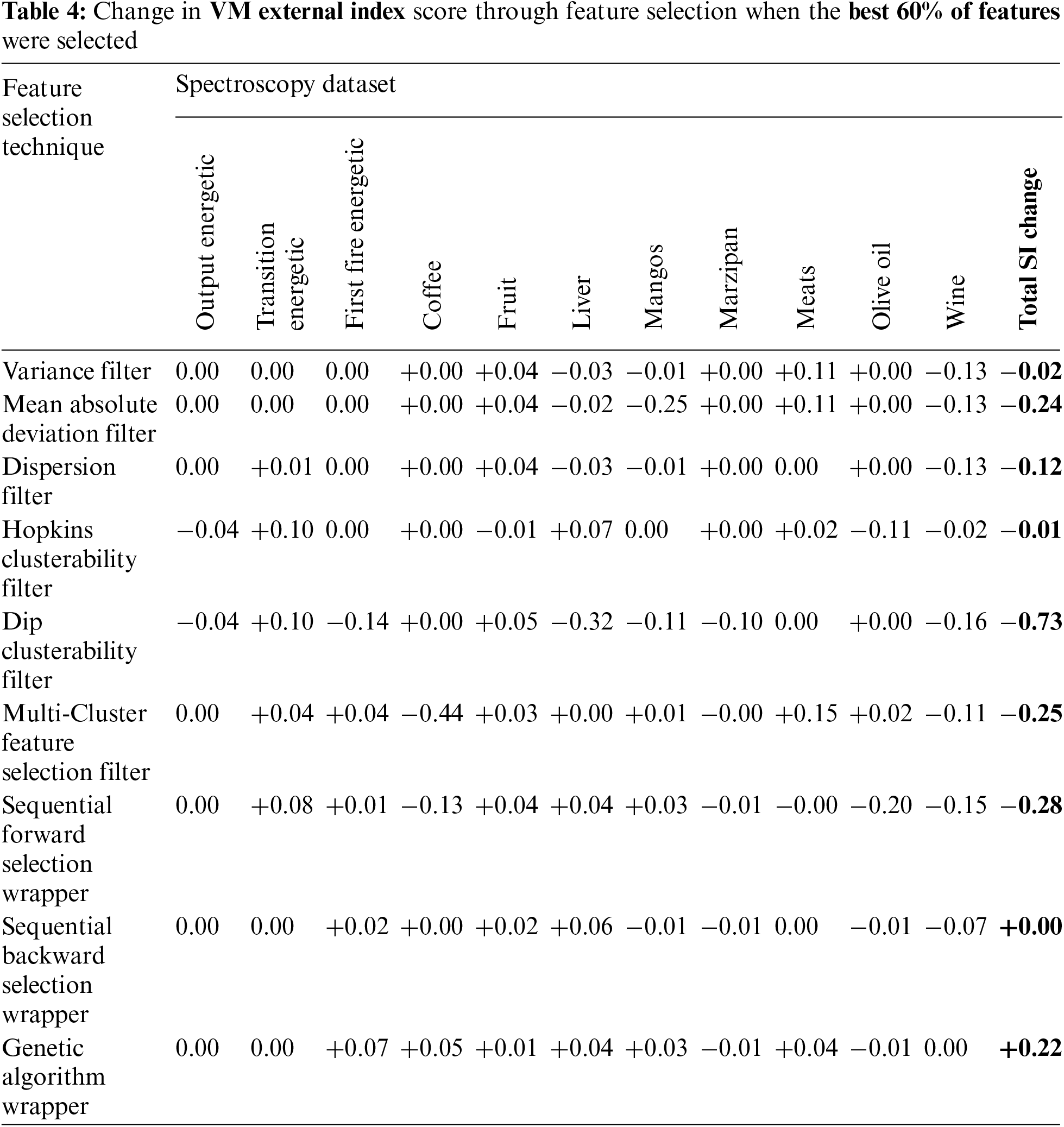
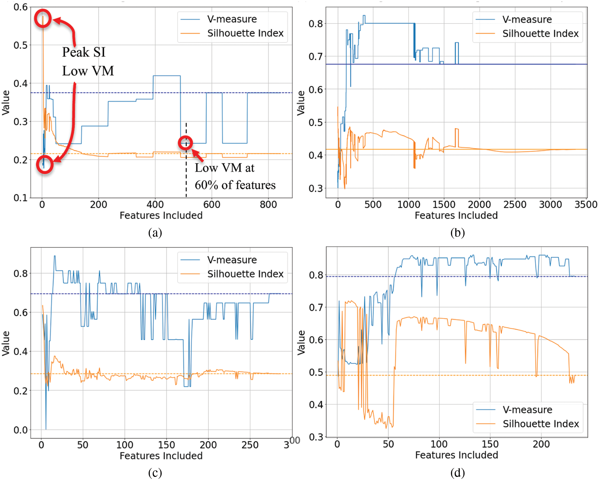
Figure 1: Exemplar plots of the internal index score (Silhouette Index) and external index score (V-measure) vs. the number of included features. The dashed lines represent the baseline scores where all features are included, i.e., no feature selection. (a) Wine FTIR data-dispersion filter (b) first fire energetic FTIR data-hopkins clusterability filter (c) coffe MIR-DRIFT data-multi-cluster feature selection (d) liver FTIR data-sequential forward selection wrapper
This presents a problem for selecting the number of features based on when the maximum SI is achieved. Often the maximum SI occurs when the number of features is very low. Selecting features based on peak SI alone will likely result in worse real-world clustering performance when assessed using labeled data and an external clustering index such as VM.
Selection based on peak VM is a better approach since this represents the most correct clustering based on the labelled data. However, this is not realistic as the prime application of cluster analysis (unsupervised learning) is when labeled data is not available. Without labels, a VM cannot be calculated.
The approach utilized by Solorio-Fernández, Carrasco-Ochoa and Martínez-Trinidad [17] where 40%, 50% or 60% of the features is now considered, along with an adjusted version where 10% is chosen due to the very high number of features in spectroscopic data. All techniques did result in improved VM scores at some point in the plots. However, due to the inconsistent nature of the results as seen in these plots, it was not possible to choose a percentage value that lead to consistently improved results. Of the options evaluated, selecting the nominal value of 60% did lead to the best results. However, as shown in Tab. 4, the results were on average still worse than doing no feature selection. An explicit example of this poor outcome is circled in Fig. 1a.
To investigate whether this phenomenon is specific to the internal and external indices chosen for this study, evaluations were done using alternative indices. Specifically, the Davies-Bouldin [59] and Calinski-Harabasz [60] internal indices were evaluated as alternatives to the Silhouette index, and the Adjusted Rand [61] and Adjusted Mutual Information [62] external indices were evaluated as alternatives to the V-measure. All resulted in similar outcomes with instability and poor external index scores at very low number of features, and inconsistent internal and external index scores across the range of features that make it difficult to select a consistently beneficial number of features.
As previously noted, the genetic algorithm was the exception to the inconsistent results from other techniques, delivering an on average positive effect on the clustering outcomes when measured using both an internal index, and an external index with labeled data. To investigate this further, the plots generated by the genetic algorithms were examined. Representative examples of these are shown in Figs. 2a–2d.
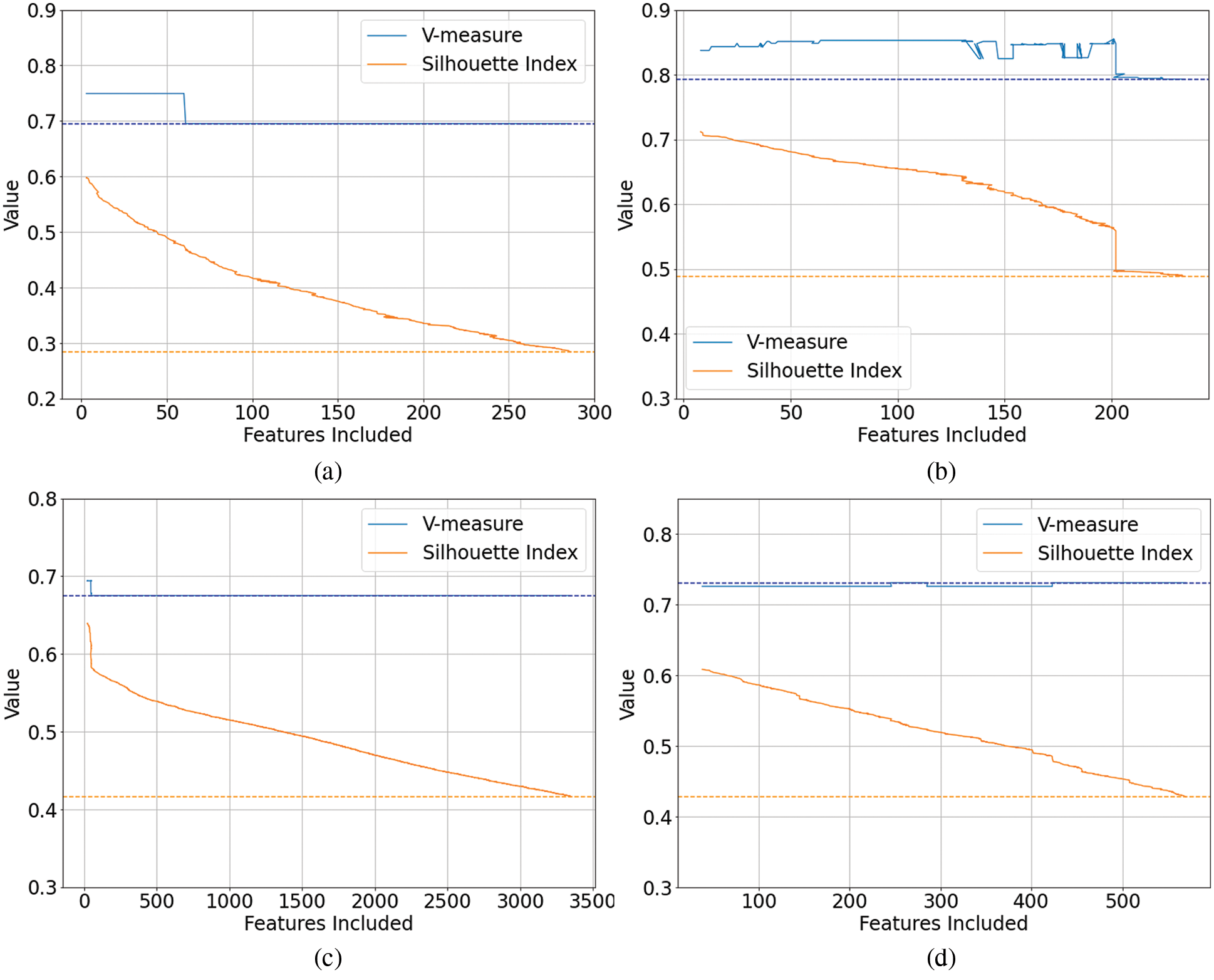
Figure 2: Genetic Algorithm feature selection plots of the internal index score (Silhouette Index) and external index score (V-measure) vs. the number of included features. The dashed lines represent the baseline scores where all features are included, i.e., no feature selection. (a) Coffee MIR-DRIFT Data-GA Feature Selection, (b) Liver FTIR Data-GA Feature Selection, (c) Transition Energetic FTIR Data-GA Feature Selection, (d) Liver FTIR-GA Feature Selection
One significant difference observed was the stability in the internal and external indices as the genetic algorithms progressed. As the internal index score (SI) was maximized through generations of the genetic algorithm and as the number of features reduced, the relationship between the internal and external indices remained consistent, including at low numbers of features. This was in stark contrast to the other techniques where a high SI score at a low number of features often resulted in very poor V-measure scores. It was also noted that while there were detrimental or negative outcomes from the genetic algorithms on two of the eleven data sets (Olive Oil and Marzipan), the negative changes were quite small (as seen in Fig. 2d).
Another attractive attribute of the genetic algorithms was that they will run until no further improvement in SI can be achieved. This natural stopping point typically achieved low numbers of features and an increase in VM was observed to occurring towards the lower number of features. This removes the need to explicitly choose the number of features for genetic algorithms, with the natural end point of the genetic algorithm likely to result in the best results.
Overall, the stability and on average positive results that come from the application of genetic algorithms indicate that genetic algorithms are the most suitable feature selection technique of those we have evaluated for cluster analysis of spectroscopy.
Feature selection presents an opportunity for improved cluster analysis results in spectroscopy. However, significant challenges were observed:
• The unlabeled data, typically high dimensionality, and low sample sizes associated with spectroscopy limit the suitability of many techniques.
• Due to the unsupervised nature of cluster analysis where it is applied to unlabeled data, evaluating and having confidence in the results when applied to unlabeled spectroscopy datasets is also challenging. This was apparent in our findings.
• And finally, determining a practical approach for selecting the number of features to choose for unlabeled datasets was a challenge for many techniques we evaluated.
In our evaluation, wrapper techniques performed better than filter techniques in feature selection for cluster analysis of our spectroscopy datasets. However, wrapper techniques are typically computationally intensive which does not match well with the high dimensionality of spectroscopy data and can lead to excessive execution time. Overall, genetic algorithms were found to be the most effective from the nine techniques evaluated. Their stable and reliable nature made them particularly attractive for our application in cluster analysis of spectroscopy.
We also proposed a new approach of Clusterability filters for feature selection in cluster analysis. Based on clusterability measures, two versions of this were implemented for evaluation; the Dip clusterability filter and the Hopkins clusterability filter. The Hopkins clusterability filter was found to be the best performing filter technique in our analysis, including better than the well-recognized Multi-Cluster Feature Selection (MCFS) technique from Cai et al. [14]. While this is a positive result for a new technique, some challenging datasets meant none of the filter techniques evaluated were consistently beneficial when averaged across the eleven spectroscopy datasets in our evaluation. It was also observed that results varied greatly for different techniques depending on the specifics of the dataset and the number of features selected. Only the genetic algorithm resulted in better results on average than utilizing the whole spectroscopy spectra and performed consistently across all datasets. These positive outcomes for the genetic algorithm wrapper method came at the expense of significant computation time.
It is also acknowledged that there are many other unsupervised feature selection techniques that have not been evaluated for our application of cluster analysis in spectroscopy. As identified in our research, it is difficult to predict which feature selection techniques will work well for specific datasets and applications without evaluation. This is true for many aspects of cluster analysis, including clustering algorithms and pre-processing techniques.
Similarly, our proposed Clusterability filters for unsupervised feature selection warrant further evaluation. We have seen that cluster analysis of spectroscopy is a challenging domain for feature selection to deliver improved results. However, cluster analysis is a widely utilized technique across a broad range of domains beyond spectroscopy and chemometrics. Here, Clusterability filters may prove to result in more significant improvements in cluster analysis outcomes. Consideration could also be given for creating a hybrid method combining the Hopkins clusterability filter (the best filter technique evaluated) with the genetic algorithm wrapper method (best wrapper technique evaluated). Using the Hopkins clusterability filter could produce a feature subset for further refinement by the genetic algorithm, reducing the execution time of the genetic algorithm while potentially still obtaining favorable results.
Funding Statement: SC's research is supported by the Commonwealth of Australia as represented by the Defence Science and Technology Group of the Department of Defence, and by an Australian Government Research Training Program (RTP) Scholarship.
Conflicts of Interest: The authors declare that they have no conflicts of interest to report regarding the present study.
References t
1. R. O. Duda, P. E. Hart and D. G. Stork, Pattern Classification, New York, USA: Wiley, 2012. [Google Scholar]
2. C. Hennig, “What are the true clusters?,” Pattern Recognition Letters, vol. 64, pp. 53–62, 2015. [Google Scholar]
3. D. J. Hand, “Discrimination and classification,” in Wiley Series in Probability and Mathematical Statistics, Chichester, USA: Wiley, pp. 155–158, 1981. [Google Scholar]
4. A. Adolfsson, M. Ackerman and N. C. Brownstein, “To cluster, or not to cluster: An analysis of clusterability methods,” Pattern Recognition, vol. 88, pp. 13–26, 2019. [Google Scholar]
5. R. G. Brereton, “Pattern recognition in chemometrics,” Chemometrics and Intelligent Laboratory Systems, vol. 149, pp. 90–96, 2015. [Google Scholar]
6. S. Crase, B. Hall and S. N. Thennadil, “Cluster analysis for IR and NIR spectroscopy: Current practices to future perspectives,” Computers, Materials & Continua, vol. 69, no. 2, pp. 1945–1965, 2021. [Google Scholar]
7. E. X. Min, X. F. Guo, Q. Liu, G. Zhang, J. J. Cui et al., “A survey of clustering with deep learning: From the perspective of network architecture,” IEEE Access, vol. 6, pp. 39501–39514, 2018. [Google Scholar]
8. Z. Xiaobo, Z. Jiewen, M. J. Povey, M. Holmes and M. Hanpin, “Variables selection methods in near-infrared spectroscopy,” Analytica Chimica Acta, vol. 667, no. 1–2, pp. 14–32, 2010. [Google Scholar]
9. R. M. Balabin and S. V. Smirnov, “Variable selection in near-infrared spectroscopy: Benchmarking of feature selection methods on biodiesel data,” Analytica Chimica Acta, vol. 692, no. 1–2, pp. 63–72, 2011. [Google Scholar]
10. J. Wan, Y. C. Chen, A. J. Morris and S. N. Thennadil, “A comparative investigation of the combined effects of pre-processing, wavelength selection, and regression methods on near-infrared calibration model performance,” Applied Spectroscopy, vol. 71, no. 7, pp. 1432–1446, 2017. [Google Scholar]
11. J. G. Dy and C. E. Brodley, “Feature selection for unsupervised learning,” Journal of Machine Learning Research, vol. 5, pp. 845–889, 2004. [Google Scholar]
12. C. Boutsidis, M. Mahoney and P. Drineas, “Unsupervised feature selection for the k-means clustering problem,” in Advances in Neural Information Processing Systems, Vancouver, British Columbia, Canada, pp. 153–161, 2009. [Google Scholar]
13. M. Dash and H. Liu, “Feature selection for clustering,” in Pacific-Asia Conf. on Knowledge Discovery and Data Mining, Berlin, Germany, pp. 110–121, 2000. [Google Scholar]
14. D. Cai, C. Zhang and X. He, “Unsupervised feature selection for multi-cluster data,” in Proc. of the 16th ACM SIGKDD Int. Conf. on Knowledge Discovery and Data Mining, Washington, DC, USA, pp. 333–342, 2010. [Google Scholar]
15. M. Dash, K. Choi, P. Scheuermann and H. Liu, “Feature selection for clustering-a filter solution,” in Proc. of the 2002 IEEE Int. Conf. on Data Mining, Maebashi City, Japan, pp. 115–122, 2002. [Google Scholar]
16. S. Alelyani, J. Tang and H. Liu, “Feature selection for clustering: A review,” in Data Clustering: Algorithms and Applications, Chapman and Hall/CRC, pp. 29–60, 2013. [Google Scholar]
17. S. Solorio-Fernández, J. A. Carrasco-Ochoa and J. F. Martínez-Trinidad, “A review of unsupervised feature selection methods,” Artificial Intelligence Review, vol. 53, no. 2, pp. 907–948, 2019. [Google Scholar]
18. J. Tang and H. Liu, “Unsupervised feature selection for linked social media data,” in Proc. of the 18th ACM SIGKDD Int. Conf. on Knowledge Discovery and Data Mining, Beijing, China, pp. 904–912, 2012. [Google Scholar]
19. E. Bertran, M. Blanco, S. Maspoch, M. C. Ortiz, M. S. Sanchez et al., “Handling intrinsic non-linearity in near-infrared reflectance spectroscopy,” Chemometrics and Intelligent Laboratory Systems, vol. 49, no. 2, pp. 215–224, 1999. [Google Scholar]
20. X. He, D. Cai and P. Niyogi, “Laplacian score for feature selection,” in Advances in Neural Information Processing Systems, Vancouver, British Columbia, Canada, pp. 507–514, 2006. [Google Scholar]
21. G. Downey, R. Briandet, R. H. Wilson and E. K. Kemsley, “Near- and mid-infrared spectroscopies in food authentication: Coffee varietal identification,” Journal of Agricultural and Food Chemistry, vol. 45, no. 11, pp. 4357–4361, 1997. [Google Scholar]
22. J. K. Holland, E. K. Kemsley and R. H. Wilson, “Use of Fourier transform infrared spectroscopy and partial least squares regression for the detection of adulteration of strawberry purees,” Journal of the Science of Food and Agriculture, vol. 76, no. 2, pp. 263–269, 1998. [Google Scholar]
23. M. Toplak, G. Birarda, S. Read, C. Sandt, S. M. Rosendahl et al., “Infrared orange: Connecting hyperspectral data with machine learning,” Synchrotron Radiation News, vol. 30, no. 4, pp. 40–45, 2017. [Google Scholar]
24. A. A. Munawar, Kusumiyati and D. Wahyuni, “Near infrared spectroscopic data for rapid and simultaneous prediction of quality attributes in intact mango fruits,” Data in Brief, vol. 27, no. 104789, 2019. [Google Scholar]
25. J. Christensen, L. Norgaard, H. Heimdal, J. G. Pedersen and S. B. Engelsen, “Rapid spectroscopic analysis of marzipan-comparative instrumentation,” Journal of Near Infrared Spectroscopy, vol. 12, no. 1, pp. 63–75, 2004. [Google Scholar]
26. O. Al-Jowder, E. K. Kemsley and R. H. Wilson, “Mid-infrared spectroscopy and authenticity problems in selected meats: A feasibility study,” Food Chemistry, vol. 59, no. 2, pp. 195–201, 1997. [Google Scholar]
27. H. S. Tapp, M. Defernez and E. K. Kemsley, “Ftir spectroscopy and multivariate analysis can distinguish the geographic origin of extra virgin olive oils,” Journal of Agricultural and Food Chemistry, vol. 51, no. 21, pp. 6110–5, 2003. [Google Scholar]
28. T. Skov, D. Ballabio and R. Bro, “Multiblock variance partitioning: A new approach for comparing variation in multiple data blocks,” Analytica Chimica Acta, vol. 615, no. 1, pp. 18–29, 2008. [Google Scholar]
29. J. Engel, J. Gerretzen, E. Szymańska, J. J. Jansen, G. Downey et al., “Breaking with trends in pre-processing?,” TrAC Trends in Analytical Chemistry, vol. 50, pp. 96–106, 2013. [Google Scholar]
30. H. Martens and E. Stark, “Extended multiplicative signal correction and spectral interference subtraction: New preprocessing methods for near infrared spectroscopy,” Journal of Pharmaceutical and Biomedical Analysis, vol. 9, no. 8, pp. 625–635, 1991. [Google Scholar]
31. A. Kohler, U. Bocker, J. Warringer, A. Blomberg, S. W. Omholt et al., “Reducing inter-replicate variation in Fourier transform infrared spectroscopy by extended multiplicative signal correction,” Applied Spectroscopy, vol. 63, no. 3, pp. 296–305, 2009. [Google Scholar]
32. S. N. Thennadil and E. B. Martin, “Empirical preprocessing methods and their impact on nir calibrations: A simulation study,” Journal of Chemometrics, vol. 19, no. 2, pp. 77–89, 2005. [Google Scholar]
33. J. Demšar, T. Curk, A. Erjavec, Č Gorup, T. Hočevar et al., “Orange: Data mining toolbox in python,” Journal of Machine Learning Research, vol. 14, no. 1, pp. 2349–2353, 2013. [Google Scholar]
34. M. Aldenderfer and R. Blashfield, “A review of clustering methods,” in Cluster Analysis, Beverly Hills, CA, USA: SAGE Publications, pp. 34–62, 1984. [Google Scholar]
35. P. Lasch, W. Haensch, D. Naumann and M. Diem, “Imaging of colorectal adenocarcinoma using FT-IR microspectroscopy and cluster analysis,” Biochimica et Biophysica Acta (BBA)-Molecular Basis of Disease, vol. 1688, no. 2, pp. 176–186, 2004. [Google Scholar]
36. N. Cebi, C. E. Dogan, A. E. Mese, D. Ozdemir, M. Arici et al., “A rapid atr-ftir spectroscopic method for classification of gelatin gummy candies in relation to the gelatin source,” Food Chemistry, vol. 277, pp. 373–381, 2019. [Google Scholar]
37. R. Tibshirani, G. Walther and T. Hastie, “Estimating the number of clusters in a data set via the gap statistic,” Journal of the Royal Statistical Society Series B-Statistical Methodology, vol. 63, no. 2, pp. 411–423, 2001. [Google Scholar]
38. P. J. Rousseeuw, “Silhouettes: A graphical aid to the interpretation and validation of cluster analysis,” Journal of Computational and Applied Mathematics, vol. 20, pp. 53–65, 1987. [Google Scholar]
39. J. Li, K. Cheng, S. Wang, F. Morstatter, R. P. Trevino et al., “Feature selection: A data perspective,” ACM Computing Surveys (CSUR), vol. 50, no. 6, pp. 1–45, 2017. [Google Scholar]
40. J. A. Hartigan and P. M. Hartigan, “The dip test of unimodality,” The Annals of Statistics, vol. 13, no. 1, pp. 70–84, 1985. [Google Scholar]
41. B. W. Silverman, “Using kernel density estimates to investigate multimodality,” Journal of the Royal Statistical Society: Series B (Methodological), vol. 43, no. 1, pp. 97–99, 1981. [Google Scholar]
42. B. Hopkins and J. G. Skellam, “A new method for determining the type of distribution of plant individuals,” Annals of Botany, vol. 18, no. 2, pp. 213–227, 1954. [Google Scholar]
43. S. Maurus and C. Plant, “Skinny-dip,” in Proc. of the 22nd ACM SIGKDD Int. Conf. on Knowledge Discovery and Data Mining, San Francisco, CA, USA, pp. 1055–1064, 2016. [Google Scholar]
44. A. Banerjee and R. N. Dave, “Validating clusters using the hopkins statistic,” in IEEE Int. Conf. on Fuzzy Systems, Budapest, Hungary, vol. 1, pp. 149–153, 2004. [Google Scholar]
45. Lachhebo/pyclustertend: Release of pyclustertend (2019). Zenodo. [Online]. Available: https://doi.org/10.5281/zenodo.3540674. [Google Scholar]
46. H. Xiong and L. Zhongmou, “Cluster validation measures,” in Data Clustering: Algorithms and Applications, Philadelphia, PA, USA: CRC Press LLC, pp. 572–602, 2013. [Google Scholar]
47. E. Rendón, I. M. Abundez, C. Gutierrez, S. D. Zagal, A. Arizmendi et al., “A comparison of internal and external cluster validation indexes,” in Proc. of the 5th WSEAS Int. Conf. on Computer Engineering and Applications, Wisconsin, United States, pp. 158–163, 2011. [Google Scholar]
48. H. Chouikhi, M. Charrad and N. Ghazzali, “A comparison study of clustering validity indices,” in Global Summit on Computer & Information Technology, Sousse, Tunisia, pp. 1–4, 2015. [Google Scholar]
49. S. Petrovic, “A comparison between the silhouette index and the davies-bouldin index in labelling IDS clusters,” in Proc. of the 11th Nordic Workshop of Secure IT Systems, Linköping, Sweden, pp. 53–64, 2006. [Google Scholar]
50. F. Pedregosa, G. Varoquaux, A. Gramfort, V. Michel, B. Thirion et al., “Scikit-learn: Machine learning in python,” Journal of Machine Learning Research, vol. 12, no. Oct, pp. 2825–2830, 2011. [Google Scholar]
51. I. Guyon and A. Elisseeff, “An introduction to variable and feature selection,” Journal of Machine Learning Research, vol. 3, no. Mar, pp. 1157–1182, 2003. [Google Scholar]
52. M. Kudo and J. Sklansky, “Comparison of algorithms that select features for pattern classifiers,” Pattern Recognition, vol. 33, no. 1, pp. 25–41, 2000. [Google Scholar]
53. J. H. Holland, “Adaptation in natural and artificial systems: An introductory analysis with applications tobiology, control and artificial intelligence,” MIT press, 1992. [Google Scholar]
54. W. Siedlecki and J. Sklansky, “A note on genetic algorithms for large-scale feature selection,” in Handbookof Pattern Recognition and Computer Vision, Singapore: World Scientific, pp. 88–107, 1993. [Google Scholar]
55. A. Niazi and R. Leardi, “Genetic algorithms in chemometrics,” Journal of Chemometrics, vol. 26, no. 6, pp. 345–351, 2012. [Google Scholar]
56. A. Remi-Omosowon and Y. Gonzalez, Pyeasyga: A Simple and easy-to-use implementation of a genetic algorithm library in Python (2014). GitHub. Accessed: Oct 2020. [Online]. Available: https://github.com/remiomosowon/pyeasyga. [Google Scholar]
57. M. J. Anzanello, F. S. Fogliatto, R. S. Ortiz, R. Limberger and K. Mariotti, “Selecting relevant Fourier transform infrared spectroscopy wavenumbers for clustering authentic and counterfeit drug samples,” Science and Justice, vol. 54, no. 5, pp. 363–368, 2014. [Google Scholar]
58. person-group-type="author">A. Rosenberg and J. Hirschberg, “V-measure: A conditional entropy-based external cluster evaluation measure,” in Proc. of the 2007 Joint Conf. on Empirical Methods in Natural Language Processing and Computational Natural Language Learning (EMNLP-CoNLLPrague, Czech Republic, pp. 410–420, 2007. [Google Scholar]
59. D. L. Davies and D. W. Bouldin, “A cluster separation measure,” IEEE Transactions on Pattern Analysis & Machine Intelligence, vol. 1, no. 2, pp. 224–227, 1979. [Google Scholar]
60. T. Calinski and J. Harabasz, “A dendrite method for cluster analysis,” Communications in Statistics - Theory and Methods, vol. 3, no. 1, pp. 1–27, 1974. [Google Scholar]
61. L. Hubert and P. Arabie, “Comparing partitions,” Journal of Classification, vol. 2, no. 1, pp. 193–218, 1985. [Google Scholar]
62. N. X. Vinh, J. Epps and J. Bailey, “Information theoretic measures for clusterings comparison: Variants, properties, normalization and correction for chance,” Journal of Machine Learning Research, vol. 11, pp. 2837–2854, 2010. [Google Scholar]
 | This work is licensed under a Creative Commons Attribution 4.0 International License, which permits unrestricted use, distribution, and reproduction in any medium, provided the original work is properly cited. |