Computers, Materials & Continua DOI:10.32604/cmc.2022.022668
Article

Two-Tier Clustering with Routing Protocol for IoT Assisted WSN

A. Arokiaraj Jovith1, Mahantesh Mathapati2, M. Sundarrajan3, N. Gnanasankaran4, Seifedine Kadry5, Maytham N. Meqdad6 and Shabnam Mohamed Aslam7,*

1Department of Networking and Communications College of Engineering and Technology, SRM Institute of Science and Technology, Kattankulathur, 603203, India
2Department of Computer Science and Engineering, Rajarajeswari College of Engineering, Bengaluru, 560074, India
3Department of Computer Science and Engineering, K. Ramakrishnan College of Engineering, Tiruchirappalli, 621112, India
4Department of Computer Science, Thiagarajar College, Madurai, 625019, India
5Department of Applied Data Science, Noroff University College, Kristiansand, Norway
6Al-Mustaqbal University College, Hillah, Iraq
7Department of Information Technology, College of Computing and Information Sciences, Majmaah University, Al Majmaah, 11952, Saudi Arabia
*Corresponding Author: Shabnam Mohamed Aslam. Email: s.aslam@mu.edu.sa
Received: 15 August 2021; Accepted: 09 October 2021

Abstract: In recent times, Internet of Things (IoT) has become a hot research topic and it aims at interlinking several sensor-enabled devices mainly for data gathering and tracking applications. Wireless Sensor Network (WSN) is an important component in IoT paradigm since its inception and has become the most preferred platform to deploy several smart city application areas like home automation, smart buildings, intelligent transportation, disaster management, and other such IoT-based applications. Clustering methods are widely-employed energy efficient techniques with a primary purpose i.e., to balance the energy among sensor nodes. Clustering and routing processes are considered as Non-Polynomial (NP) hard problems whereas bio-inspired techniques have been employed for a known time to resolve such problems. The current research paper designs an Energy Efficient Two-Tier Clustering with Multi-hop Routing Protocol (EETTC-MRP) for IoT networks. The presented EETTC-MRP technique operates on different stages namely, tentative Cluster Head (CH) selection, final CH selection, and routing. In first stage of the proposed EETTC-MRP technique, a type II fuzzy logic-based tentative CH (T2FL-TCH) selection is used. Subsequently, Quantum Group Teaching Optimization Algorithm-based Final CH selection (QGTOA-FCH) technique is deployed to derive an optimum group of CHs in the network. Besides, Political Optimizer based Multihop Routing (PO-MHR) technique is also employed to derive an optimal selection of routes between CHs in the network. In order to validate the efficacy of EETTC-MRP method, a series of experiments was conducted and the outcomes were examined under distinct measures. The experimental analysis infers that the proposed EETTC-MRP technique is superior to other methods under different measures.

Keywords: Wireless networks; internet of things; energy efficiency; clustering; multi-hop routing; metaheuristics

1  Introduction

In the recent years, the field of microelectronics has become highly advanced which led to research and development of resource-constraint devices, small nodes, and low-cost wireless sensors. Wireless Sensor Networks (WSNs) play a vital role in several WSN-enabled IoT applications [1]. WSN-enabled IoT devices have been applied in a wide range of domains such as industrial wireless network, smart parking system, border security monitoring, animal monitoring system, and healthcare observing scheme [2]. Actuation, Radio Frequency Identification (RFID), Sensor Nodes (SN), and other such devices are integrated to create WSN-enabled IoT networks so as to achieve few general objectives. The nodes that form a part of WSN-enabled IoT make the physical objects aware about real-time features in the positioned networks like monitoring, hearing, triggering and feeling an event with co-ordination of another device [3]. The data collected from sensors is then transferred to Base Station (BS) through routing protocol. Almost all the devices that form a part of WSN-enabled IoT network operates on constrained non-rechargeable energy sources like battery. In general, WSN-enabled IoT applications are positioned in dense and rugged environments, and it can be complex to add/exchange the energy source from sensors. Hence, effective energy management is a major problem in WSN-enabled IoT devices [4]. Fig. 1 illustrates the structure of WSN.

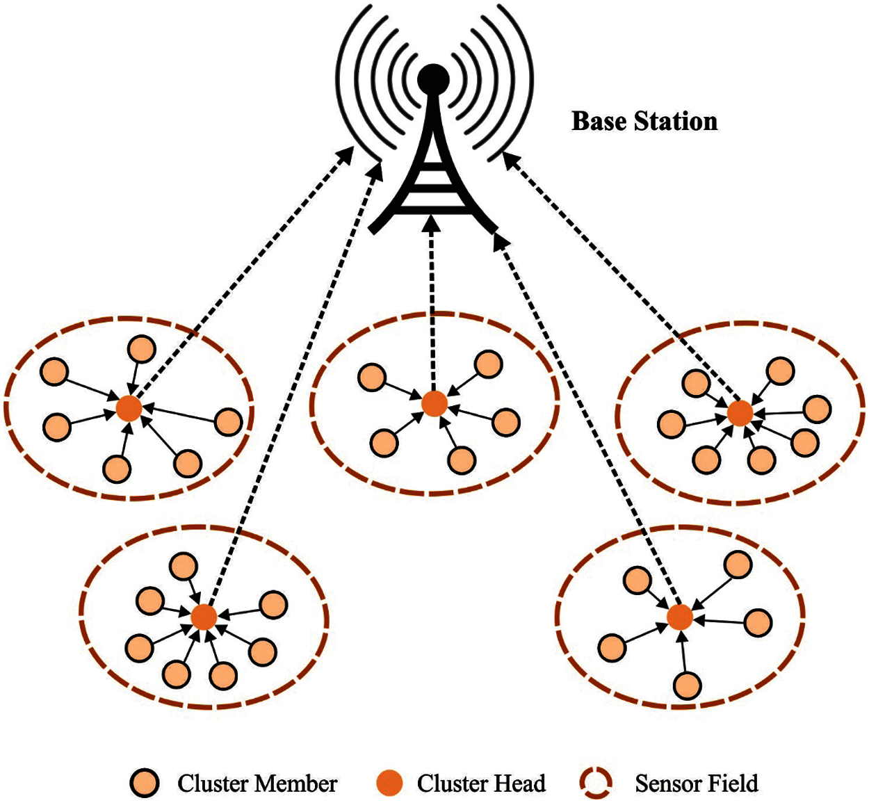
Figure 1: Structure of WSN

WSN-enabled IoT network is positioned at a wide range compared to WSNs. Further, the number of nodes (mainly resource constraints) is larger than WSN networks [5]. Therefore, conventional WSN approaches may not be efficient for scalable WSN-enabled IoT networks. In order to overcome the issues pertaining to network lifetime and scalability, several authors adapted cluster-based hierarchical architecture [6]. The main objective in cluster-based routing protocol is the selection of effective Cluster Head (CH) and organization of residual nodes in the cluster. The node, within the clusters, transmits the data to CH. Here, CHs have a responsibility towards the aggregated data of local Cluster Members (CM) and it transmits the collected data to BS or nearby CH towards the BS. This further constrains the CHs which results in additional energy depletion than average node [7]. The CH, closer to BS, consumes their energy quickly than other nodes since it performs as Relay Node (RN) for data aggregation, transmitted with distant CH.

In all cases, WSN BS should generate an aggregate value for end users. It is possible to increase the level of data transmission by decreasing vitality utilization and broadcast overhead [8]. The network could be appropriate in slight gathering to assist the collection of data called clusters. In data gathering, clustering could be deliberated as a partition of hub on the principles of scheme. Hence, clustering has become an attractive option to enhance the lifespan of network. There have been substantial metrics proposed earlier to evaluate the performance of a sensor organization [9]. The flexibility of the controlled systems and energy efficiency must be grouped together. The networks should be allotted with more portions based on the requirement to increase the border of the network. Member node is used here which acts as a substitute hub to send and detect the collected data to CH [10].

In Nalluri et al. [11], a hybrid protocol named EECAO protocol was presented to increase the efficiency of sensor networks in WSN-enabled IoT environment. Hybrid protocols include different clustering features like channel consistency, cognitive sensor throughput, energy cost for CH selection and a newly dispersed clustering method developed for self-organizing the positioned SN. Tandon et al. [12] proposed BiHCLR protocols to achieve energy preservation and effective routing in WSN-enabled IoT. At first, the positioned sensors are organized through a network based on network-based routing approach. Next, in order to assist the energy preservation in BiHCLR, FL algorithm is executed to select the CH for each cell in the network. At last, hybrid and biologically-inspired algorithms are employed in the selection of routing paths. The hybrid approach integrates SSO and moth search methods. In Mydhili et al. [13], the new MSPK++ clustering approach, using balanced clustering, was presented. The approach was further enhanced with the help of ML algorithm which is applicable for WSN on IoT environments.

Chouhan et al. [14] introduced multipath routing protocols with the presented optimization approach i.e., TSGWO approach in IoT-enabled WSN networks. Using multi-path routing protocols, a multi-path is developed by multi-path source nodes to many destinations. Initially, the node in IoT-enabled WSN network is inspired together and execute the CH election through FGSA approach. Further, multipath routing processes are made based on the presented TSGWO approach, where the routing path is elected, by taking the fitness variables into account, such as trust factors and QoS parameters. Shukla et al. [15] presented SEEP algorithm to leverage multihop hierarchical routing system to minimize the utilization of power. In order to attain energy-effective and scalable networks, SEEP applies a multitier-based clustering architecture. The network areas in SEEP are separated into different areas using the presented sub-region division algorithms. Each area is separated into specific amount of clusters (sub-regions). The amount of clusters gets improved toward the BS, while the area widths get minimized. Multi-hop routing and clustering are classical techniques used for improving energy efficacy of the network. Instead of letting all the nodes in the network to directly transmit the data to BS, they are collected at distinct clusters. Depending on certain benchmarks, CH nodes are elected in all the clusters. The CH nodes would collect the data from other CM nodes and then transmits the processing data to BS through multiple hops with another CH node. There are two-fold benefits present in this system. Initially, the CH nodes can compress the data gathered from CMs to decrease the pointless redundancy. Next, energy efficacy gets considerably enhanced by letting each node from the network send for adjacent CH nodes and restraining multi-hop transmission to CH node.

The current research paper designs an Energy Efficient Two-Tier Clustering with Multi-hop Routing Protocol (EETTC-MRP) for IoT networks. The presented EETTC-MRP technique operates on different stages namely, tentative Cluster Head (CH) selection, final CH selection, and routing. The proposed EETTC-MRP technique uses type II fuzzy logic-based tentative CH (T2FL-TCH) selection in its first stage. Subsequently, Quantum Group Teaching Optimization Algorithm-based Final CH selection (QGTOA-FCH) technique is used to derive an optimum set of CHs from the network. Besides, the Political Optimizer-based Multihop Routing (PO-MHR) technique is employed to perform an optimal selection of routes between CHs in the network. A widespread experimental analysis was conducted and the outcomes were inspected under different evaluation parameters.

2  The Proposed Model

In this study, a new EETTC-MRP technique is designed to achieve energy efficiency in IoT-assisted WSN. The proposed EETTC-MRP technique encompasses three major processes namely, T2FL-TCH, QGTOA-FCH, and PO-MHR. The working mechanisms of these three modules are given in subsequent sections.

2.1 System Model

WSN has several SNs and BS. The sensor network possesses the following properties [16].

•   Every node is heterogeneous. The nodes are arbitrarily allocated with sensor domain.

•   All the nodes have unique ID and it could not be transferred after it is utilized.

•   BS tend to exist outside the network too.

•   BS is a constant power supply and it has no energy constraint.

•   Node and BS are static and considered to be inactive.

•   The communication amongst SNs takes place via multi-hop symmetric communication.

•   SNs are connected with GPS devices and are location-aware.

2.2 Design of T2FL-TCH Technique

At this stage, the TCHs in IoT-assisted WSN can be proficiently chosen with the help of T2FL technique. T2FL generates effective outcomes over T1FL method. Three fuzzy input variables are considered to select the tentative CH. The three input variables are nothing but three Membership Functions (MF) each. The fuzzy set signifies three input variables, for instance, residual battery power, Distance to BS (DBS), and concentration. The linguistic variables for fuzzy sets are less, medium, and high while in case of Triangular MF (TMF), it is regarded as less, medium, and high. The 3rd fuzzy input variable has been concentrated heavily, which implies that several sensor nodes exist in specific locality. The degree of MF is demonstrated numerically compared to all other MFs.

Rule Base and Inference Engine

In this method, 27 rules are utilized based on fuzzy inference approach. Here, the rules for the procedure are discussed. X, Y, Z and C are considered here while X refers to residual battery power, Y implies DBS, Z demonstrates concentration, and C signifies the Confidence Factor (CF). The CF value that exists in CH is computed with the help of Mamdani's Fuzzy rule, assuming three input parameters such as residual battery power, DBS, and concentration. T1FL technique has four components such as fuzzifier, fuzzy inference engine, fuzzy rules, and defuzzifier. There are four steps required to complete the procedure [17]. Here, T1FL is utilized to handle the uncertainty levels to any extent, but not entirely as Type-1 fuzzy sets (T1FS) since the latter is certain about the outcomes. Conversely, Type-2 Fuzzy Logic (T2FL) approach has been helpful in circumstances when it turns out to be complex to determine a particular numeric MF and there is measurement uncertainty. The idea is to implement T2FL on WSN that is used for selecting an effectual CH. So, the load is allocated evenly amongst the SN. T2FL is considered by higher MF as well as inferior MF. These two functions are demonstrated (everyone) by T1FS MF. The interval between these two functions signifies the Footprint Of Uncertainty (FOU) that is employed for characterizing T2FL set. Assume that FOU is written as f. If f° [0, 1], and f→0, then MF is regarded as T1FL. When f→0 to 1, next T2FL becomes a varied range of FOU amongst [0, 1]. However, the formation of rules is similar to T1FL. Hence, it is written as follows.

Type2FL=PrincipalMF(Type1FL)+FOU(1)

The rules are resultant from the equation provided in Eq. (2):

CF=∑05⁡RBP+∑05⁡DistancetoBS+∑05⁡Concentration(2)

2.3 Design of QGTOA-FCH Technique

Once the TCHs are elected, QGTOA technique is applied to select FCHs. A new GTOA approach is employed based on the inspiration from a group teaching method. The acquaintance of entire class (c) could be enhanced, i.e., fundamental concept behind the presented method i.e., GTOA can be used to enhance the outcomes. In order to execute GTOA algorithm for the optimization method, an easy group teaching method is proposed according to the rules given below.

a. The only variance among students is their ability to acquire knowledge. The greatest challenge for a teacher is to formulate the teaching plans that suits the needs of learners who have different knowledge acquisition capacity.

b. The aim of a qualified teacher is to show more interest upon the student with poor capacity of acquiring knowledge.

c. Through self-learning, or interaction with fellow students, students are able to develop their knowledge in their free time.

d. To enhance the knowledge of students, decent teacher allocation methods are very useful.

Ability Grouping

In order to represent the knowledge of entire class, standard distribution functions have been employed which are expressed in Eq. (3).

f(x)=12πδexp(x−μ)2(3)

In which χ represents the value, where standard distribution functions are needed. μ denotes the mean and δ signifies the SD. In GTOA algorithm, each student is separated into two groups [18]. Outstanding group is a group of students who have optimum capacity for grasping knowledge, while the groups with poor capacity of grasping knowledge is known as average group.

Teacher Phase

In this stage, students learn about the teacher, i.e., the 2nd rule is determined before. In GTOA, the teacher generates distinct plans for outstanding group and average group.

Teacher phase I:

The teachers focus more on developing the knowledge of entire class, owing to good capability of the students in terms of knowledge acquisition. The students who belong to outstanding group possess high possibility of increasing their knowledge acquisition skills as shown in Eq. (4).

Xteacher−jt+1=Xjt+a×(Tt−F×(B×Mt+c×Xjt))(4)

Mt=1N(5)

b+c=1(6)

Here, the number of students is denoted by N,Xj denotes the knowledge of every student, T indicates the knowledge of teacher and M signifies the mean group knowledge. The teacher factor is denoted by F, Xteacher−j denotes the knowledge of student j who is taught by the teacher. Arbitrariness is presented as b whereas c denotes the interval between zero and one.

Teacher phase II:

According to the 2nd rule, the teachers shed more focus upon average group owing to weak acceptance knowledge capability of the students. The average, of the students combined together, who could attain knowledge is shown in Eq. (7).

Xieacher,jt+1=Xjt+2×d×(Tt−Xjt)(7)

Here, d represents arbitrariness in the range of zero and one. Eq. (8) addresses the problems for which a student could not gain knowledge from the teacher stage.

Xieacher,jt+1={Xteacher,j′tf(Xieacher,jt+1)<f(Xjt)Xjt,f(Xteacher,jt+1)≥f(Xjt)(8)

Student Phase

In free time, student could attain knowledge through self-learning, or interaction with classmates. This is expressed arithmetically in Eq. (9). The student stage is linked with 3rd rule by adding the student phases, I & II.

Xteacher,jt+1={Xteacher,jt+e×(Xteacher,jt+1−Xteacher,kt+1)+g×(Xteacher,jt+1−Xjt),f(Xteacher,jt+1)<f(Xteacher,kt+1)Xieacher,jt−e×(Xieacher,jt+1−Xieacher,kt+1)−g×(Xieacher,jt+1−Xjt),f(Xieacher,jt+1)≥f(Xieacher,kt+1)(9)

Here, e & g correspond to two ransom numbers in the range of zero and one, Xstudent,jt+1 represents the knowledge of student i, and Xteacher,jt+1 denotes the knowledge of student j who learns from the teacher. If students could not attain knowledge in this stage, then they can be tackled in Eq. (10).

Xjt+1={Xteacher,j′tf(Xieacher,jt+1)<f(Xstudent,jt)Xsiudeni,j′tf(Xteacher,jt+1)≥f(Xsiudeni,jt)(10)

Teacher Allocation Phase

To enhance the knowledge of students, a decent teacher allocation approach is important, which can be determined as 4th rule. The top three students are elected stimulated by the hunting behaviors of grey wolves as shown in Eq. (11).

T={xfirst′tf(Xfirstt)≤f(Xfirstt+Xsecondt+Xthirdt3)Xfirstt+Xsecondt+Xthirdt3>f(Xfirstt+Xsecondt+Xthirdt3)(11)

Here, Xfirstt,Xsecond′t and Xthirdt indicate top three best students, correspondingly.

QGTOA technique is derived based on the concept of Quantum Computing (QC) to improve the performance of GTOA. QC is a new variety of computing process that accepts the approaches associated with quantum theory as quantum entanglement, quantum measurement, and state superposition. Qubit is an essential unit of QC. The two fundamental conditions |0⟩ and |1⟩ denote the qubit which is expressed as linear combination of these two fundamental situations as follows

|Q⟩=α|0⟩+β|1⟩.(12)

|α|2 implies the probabilities of detecting state |0⟩, |β|2 refers to the probabilities of noticing state |1⟩, where |α|2+|β|2=1. The quantum has been established of n qubits. According to the nature of quantum superposition, every quantum has 2n feasible values. A n-qubits quantum is referred to as follows.

Ψ=∑x=02n−1⁡Cx|x⟩,∑x=02n−1⁡|Cx|2=1.(13)

The quantum gates have altered the condition of qubits like rotation gate, NOT gate, Hadamard gate, etc. The rotation gate [19] is described as a mutation operator for making quanta approach as the optimum solution and at last, the global optimal solutions are defined.

The rotation gate is determined as follows.

[αd(t+1)βd(t+1)]=[cos(△θd)−sin(△θd)sin(△θd)cos(△θd)][αd(t)βd(t)]ford=1,2,…,n.(14)

△θd=△×S(αd,βd), △θd signifies the rotation angle of qubit, where △ and S(αd,βd) denote size as well as way of rotation correspondingly.

During energy utilization, cluster development plays an important role. This work utilizes QGTOA clustering technique for the formation of clusters. The cluster count (k) is evaluated with the formula given below.

k=n2πεfsεmpDxBS2,(15)

where n implies the amount of SNs, D refers to the dimension of network field, and average distance of every SN to BS is represented by xBS.

By utilizing Euclidean distance, the distance between the SNs to all cluster centers is determined based on the formula given below.

Xn2CC=∑j=1N⁡(Xj−XCC),(16)

where Xn2CC represents the distance of node to cluster center, Xj implies the co-ordinate of SN j, and XCC refers to the co-ordinate of cluster centers.

2.4 Design of PO-MHR Technique

During routing process, PO-MHR technique is used to derive an optimal set of routes to BS. PO algorithm is stimulated by western political optimization method that includes two features. The initial assumptions are as follows; each citizen tries to improve their goodwill to win the election and every party attempts to attain additional seats in the parliament. PO has six stages namely, party switching, election campaign, parliamentary affairs, interparty election, constituency allocation, and party formation [20]. Fig. 2 illustrates the flowchart of PO technique.

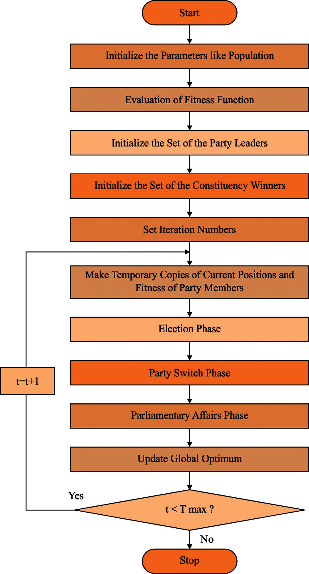
Figure 2: Flowchart of PO

The overall population could be separated to n political party, as given in Eq. (17).

P={P1,P2,P3,…,Pn}(17)

Each party includes n party members as shown in Eq. (18).

Pi={pi1,pi2,pi3,…,pin}(18)

Every party member induces d dimension as given as Eq. (19).

pij=[pi,1j,pi,2j,pi,3j,…,pi,dj]T(19)

Every solution could be an election candidate. Assume an n electoral district as denoted in Eq. (20).

C={C1,C2,C3,…,Cn}(20)

Suppose there is n member in every constituency, as given in Eq. (21).

cj={p1j,p2j,p3j,…,pnj}(21)

The party leaders are determined as the member using an optimal fitness in a party can be demonstrated as Eq. (22).

q=argmin1≤j≤nf(p1j),∀iε{1,…,n}(22)

Each party leader could be shown in Eq. (23).

P∗={p1∗,p2∗,p3∗,…,pn∗}(23)

The winner of the distinct constituencies is known as Member of Parliament, as expressed in Eq. (24)

C={c1∗,c2∗,c3∗,…,cn∗}(24)

During election campaign phase, Eqs. (25) and (26) are used to update the location of possible solutions.

pi,kj(z+1)={ifpi,kj(z−1)≤pi,kj(z)≤m∗orpi,kj(z−1)≥pi,kj(z)≥m∗,m∗+r(m∗−pi,kj(z));ifpi,kj(z−1)≤m∗≤pikj(z)orpi,kj(z−1)≥m∗≥pi,kj(z),m∗+(2r−1)|m∗−pi,kj(t)|;ifm∗≤pi,kj(z−1)≤pi,kj(z)orm∗≥pi,kj(z−1)≥pi,kj(z),m∗+(2r−1)|m∗−pikl(z−1)|;(25)

pi,kj(z+1)={ifpi,kj(z−1)≤pi,kj(z)≤m∗orpi,kj(z−1)≥pi,kj(z)≥m∗,m∗+(2r−1)|m∗−pi,kj(z)|;ifpi,kj(z−1)≤m∗≤pi,kj(z)orpi,kj(z−1)≥m∗≥pi,kj(z),pi,kj(z−1)+r(pi,kj(z)−pi,kj(z−1));ifm∗≤pi,ki(z−1)≤pi,kj(z)orm∗≥pi,kj(z−1)≥pi,kj(z),m∗+(2r−1)|m∗−pi,kj(z−1)|;(26)

In order to create a balance between exploitation and exploration, party switching is adapted. An adaptive variable λ is employed, i.e., to dramatically reduce from 1 to 0 during whole iterative process. Every candidate is elected based on the likelihood, λ and is replaced by the worst member of an arbitrarily elected party, as expressed in Eq. (27).

q=argmaxi≤j≤n⁡f(pij)(27)

During election phase, a constituency announces winner as expressed in Eq. (28).

q=argmini≤j≤n⁡f(pij)(28)

In this stage, the accessible paths between BS and CH nodes are initiated as primary population for the optimization algorithm. At first, one of the CHs is deliberated as transmitter and another CH is deliberated as intermediate sink/path. Hence, in this initialization stage, each potential path between CH and sink is expressed as follows (29).

Sol=Pi,i=1,2,…,N.(29)

Whereas, ‘Sol’ indicates the primary population set, ‘Pi’ represents the ith path between sink and CH, ‘N’ denotes the overall amount of paths. The paths include overall energy and distance.

P={RE,DIST}(30)

Let ‘RE’ be the residual energy of node in the path and ‘DIST’ means the overall distance of the path. The SD for remaining energy (σRE) is employed to measure the quality of uniform load distributions between sensors as follows (30).

RE=f1=σRE=1n∑i=1n⁡{μRE−e(nodej)}2(31)

Now,

In which, ‘n’ denotes the overall number of nodes present in the path and ‘E(nodej)’ signifies the remaining energy of ith node in the path. Next, the distance between transmitter CH and the sink is computed by the amount of Euclidean distance among every CH in the path and is expressed through Eq. (32).

DIST=∑in−1⁡(CHi(x)−CHi+1(x))+(CHi(y)−CHi+1(y))(32)

Here, ‘CHi(x)’ and ‘CHi(y)’ characterize x & y coordinates of ith CH in the path correspondingly. Therefore, the initial objective of the presented optimization is to reduce the energy consumption as expressed in (31). The next objective is to decrease the path distance which is expressed in (32). Therefore, these two variables of each path are initiated as the primary population.

In this stage, the fitness of each solution or path between the sink and CH is computed. The main goal of optimization is to discover the path with short distance and less power utilization. Therefore, the objective function consists of distance of each path and energy consumed. FF is equated as minimalization function and is a product of distance and energy as shown in Eq. (33).

Fi=min{REi×DISTi}(33)

Here, ‘Fi’ denotes the fitness of ith population, ‘REi’ represents the energy needed in ith population and ‘DISTi’ indicates the overall distance of ith population/path.

3  Performance Validation

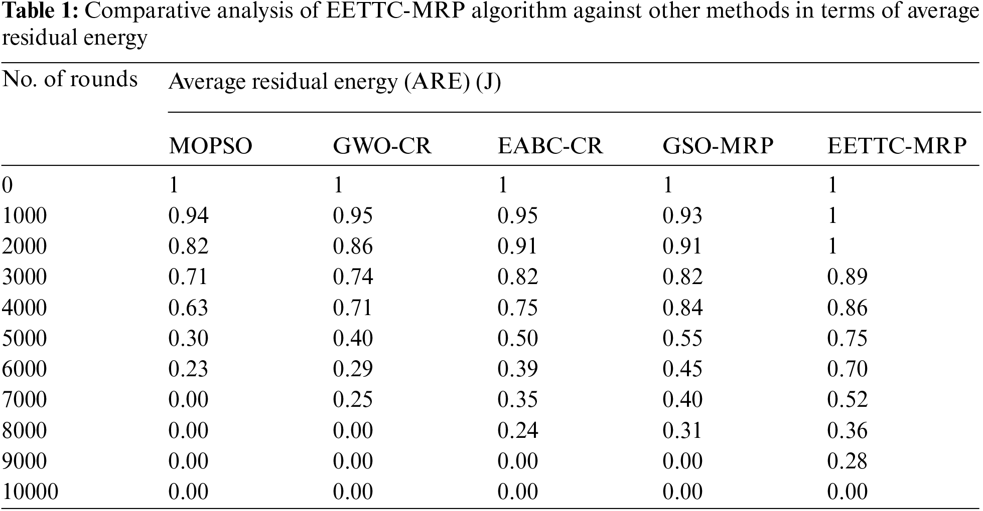
The performance of the proposed EETTC-MRP approach with respect to ARE under varying node counts was validated and the results are shown in Tab. 1 and Fig. 3. The outcomes exhibit that EETTC-MRP method attained the maximal ARE under all node counts over other techniques. For instance, with 1000 nodes, EETTC-MRP method gained a superior ARE of 1 J, whereas other methods such as MOPSO, GWO-CR, EABC-CR, and GSO-MRP achieved minimum ARE values such as 0.94, 0.95, 0.95, and 0.93 J respectively. Likewise, with 4000 nodes, EETTC-MRP method attained an increased ARE of 0.86 J, whereas MOPSO, GWO-CR, EABC-CR, and GSO-MRP techniques gained lesser ARE values such as 0.63, 0.71, 0.75, and 0.84 J respectively. In the meantime, with 6000 nodes, the proposed EETTC-MRP approach attained a high ARE of 0.70 J, whereas other techniques such as MOPSO, GWO-CR, EABC-CR, and GSO-MRP methods obtained low ARE values such as 0.23, 0.29, 0.39, and 0.45 J respectively. Simultaneously, at 7000 nodes, the presented EETTC-MRP technique attained a high ARE of 0.52 J, whereas MOPSO, GWO-CR, EABC-CR, and GSO-MRP techniques obtained the least ARE values such as 0.00, 0.25, 0.35, and 0.40 J correspondingly. Finally, with 8000 nodes, EETTC-MRP method obtained a superior ARE value of 0.36 J, whereas MOPSO, GWO-CR, EABC-CR, and GSO-MRP approaches reached minimal ARE values such as 0.00, 0.00, 0.24, and 0.31 J respectively.

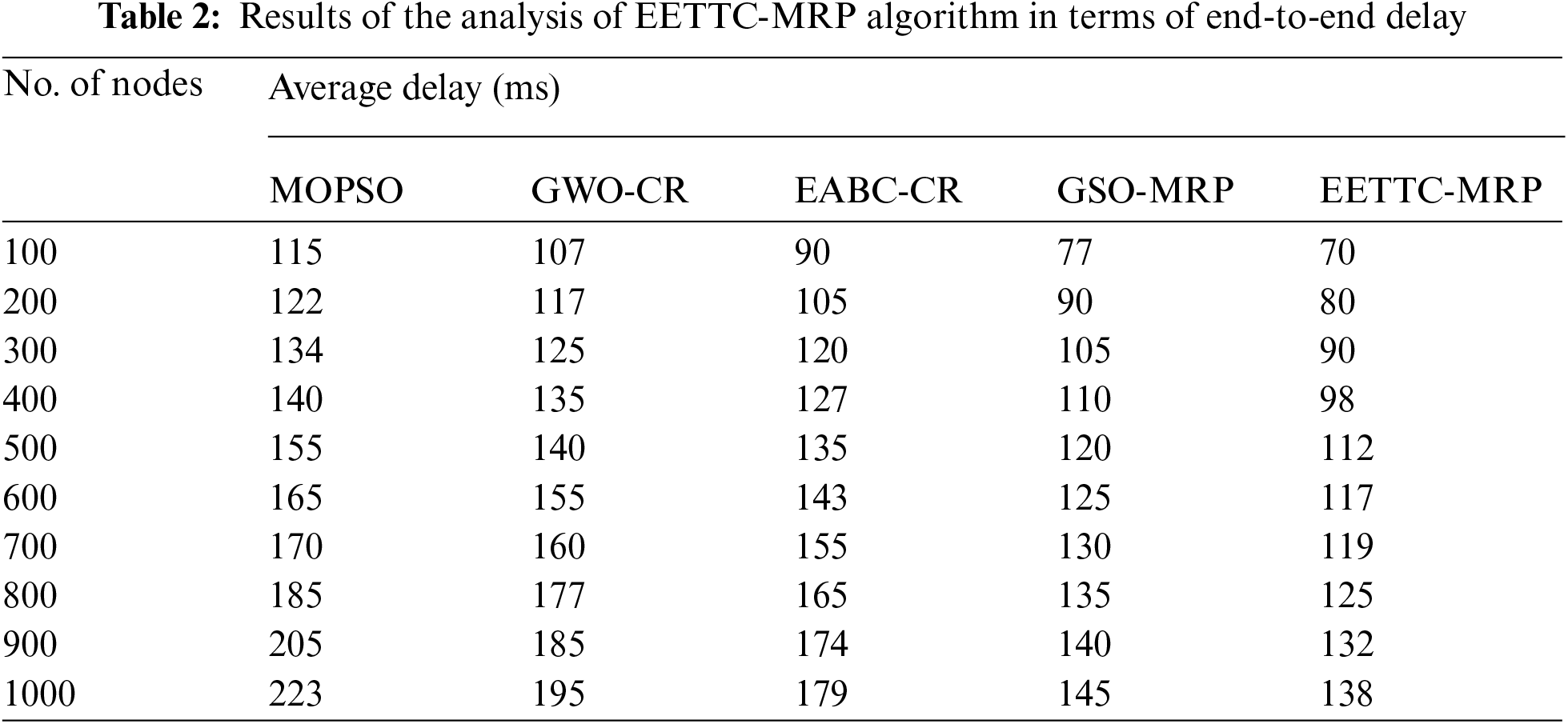
Tab. 2 and Fig. 4 provide the results for ETE delay analysis of the proposed EETTC-MRP technique against existing techniques. The results demonstrate that the presented EETTC-MRP technique accomplished superior performance with least ETE delay under several nodes. For instance, under 100 nodes, the proposed EETTC-MRP technique resulted in a reduced ETE delay of 70 ms, while MOPSO, GWO-CR, EABC-CR, and GSO-MRP techniques attained high ETE delay times such as 115, 107, 90, and 77 ms respectively. Also, under 400 nodes, the presented EETTC-MRP approach achieved a less ETE delay of 98 ms, while other techniques such as MOPSO, GWO-CR, EABC-CR, and GSO-MRP achieved high ETE delay time such as 140, 135, 127, and 110 ms correspondingly. Besides, under 600 nodes, EETTC-MRP model caused a minimal ETE delay of 117 ms, while MOPSO, GWO-CR, EABC-CR, and GSO-MRP techniques achieved improved ETE delay times such as 165, 155, 143, and 125 ms correspondingly. Additionally, under 800 nodes, EETTC-MRP method accomplished a less ETE delay of 125 ms, while MOPSO, GWO-CR, EABC-CR, and GSO-MRP techniques obtained maximal ETE delay of 185, 177, 165, and 135 ms correspondingly.

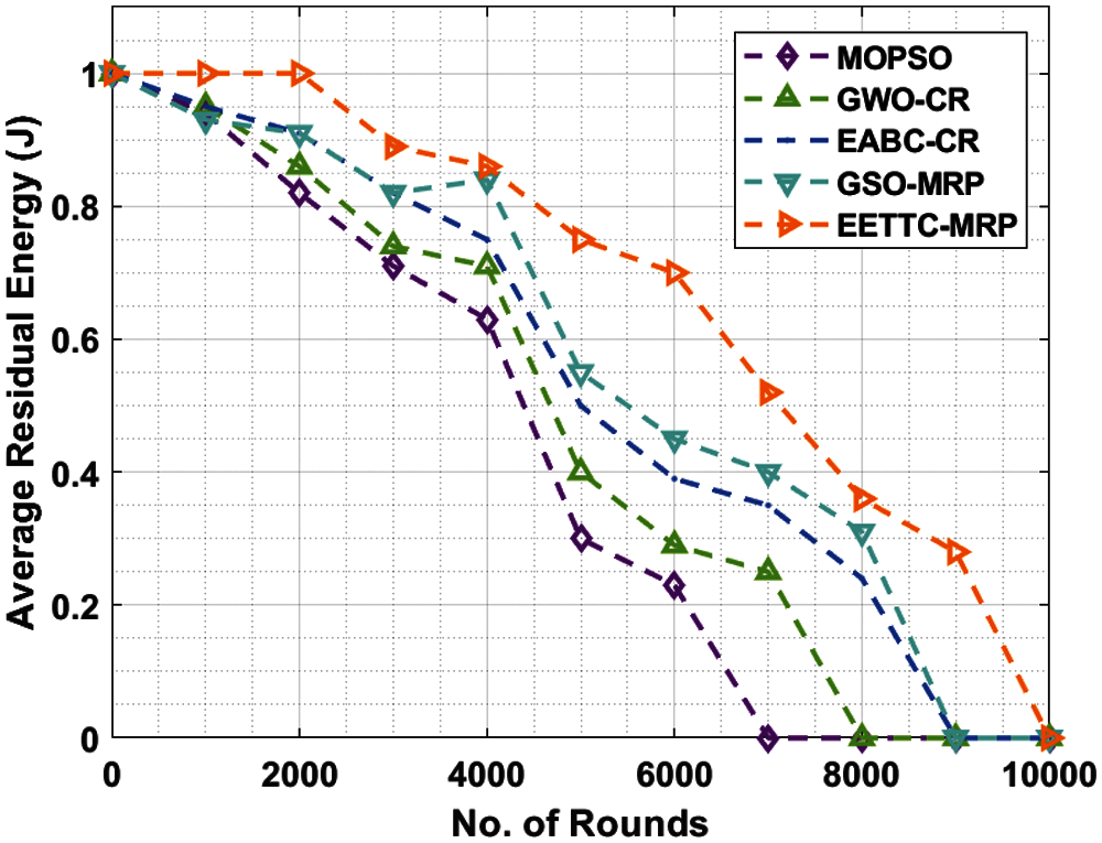
Figure 3: Average residual energy analysis of EETTC-MRP algorithm

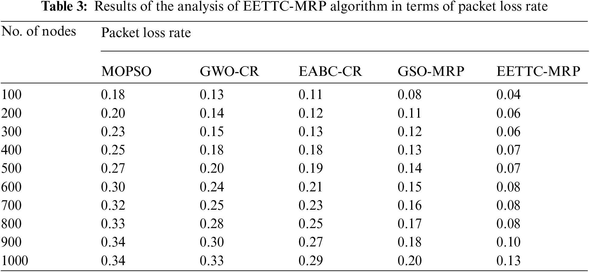
Tab. 3 and Fig. 5 offer the results of PLR analysis of the proposed EETTC-MRP approach against existing techniques. The results confirm that the presented EETTC-MRP method outperformed other methods by achieving maximum performance with less PLR under different nodes. For instance, under 100 nodes, EETTC-MRP method achieved a low PLR of 0.04, but MOPSO, GWO-CR, EABC-CR, and GSO-MRP techniques obtained high PLR values such as 0.18, 0.13, 0.11, and 0.08 correspondingly. Followed by, under 400 nodes, EETTC-MRP algorithm accomplished a less PLR of 0.07, but other techniques such as MOPSO, GWO-CR, EABC-CR, and GSO-MRP techniques gained high PLR values such as 0.25, 0.18, 0.18, and 0.13 respectively. In addition, under 600 nodes, the proposed EETTC-MRP technique achieved a low PLR of 0.08, but the presented MOPSO, GWO-CR, EABC-CR, and GSO-MRP techniques attained high PLR values such as 0.30, 0.24, 0.21, and 0.15 respectively. Furthermore, under 800 nodes, the EETTC-MRP approach accomplished a minimum PLR of 0.08 whereas the existing techniques such as MOPSO, GWO-CR, EABC-CR, and GSO-MRP attained high PLR values such as 0.33, 0.28, 0.25, and 0.17 correspondingly.

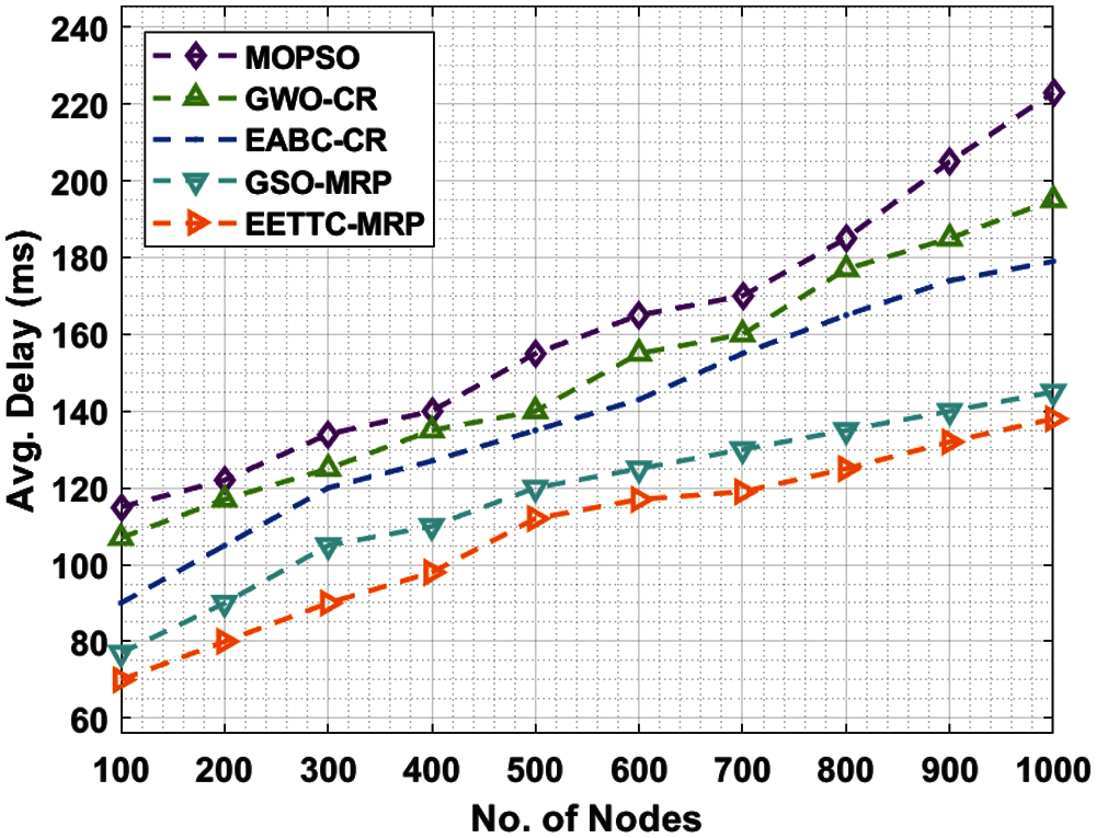
Figure 4: Average delay analysis of EETTC-MRP algorithm

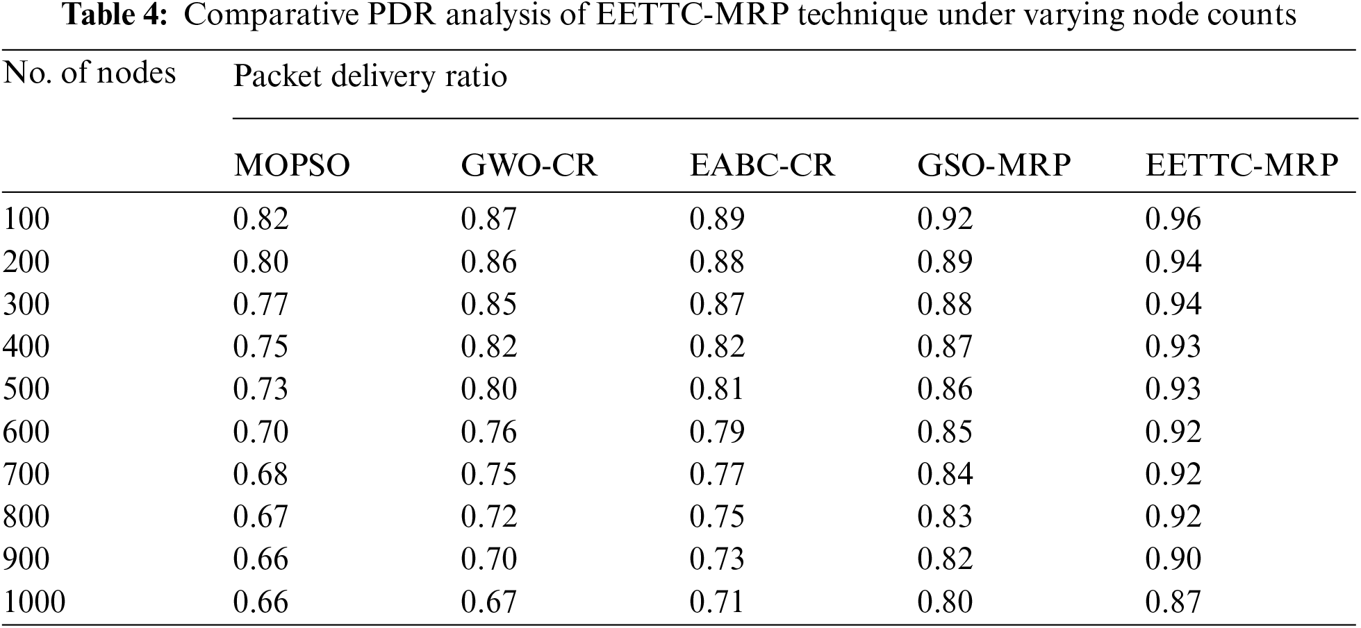
The performance of the proposed EETTC-MRP technique, in terms of PDR, under different node count is shown in Tab. 4. The results depict that the presented EETTC-MRP technique achieved a high PDR under all node counts compared to other methods. For instance, with 100 nodes, the EETTC-MRP technique attained an increased PDR of 0.96, whereas other techniques such as MOPSO, GWO-CR, EABC-CR, and GSO-MRP obtained low PDR values such as 0.82, 0.87, 0.89, and 0.92 respectively. In line with this, with 400 nodes, EETTC-MRP model reached a maximum PDR of 0.93, whereas MOPSO, GWO-CR, EABC-CR, and GSO-MRP methodologies gained less PDR values such as 0.75, 0.82, 0.82, and 0.87 correspondingly. Meanwhile, with 600 nodes, the EETTC-MRP method attained high PDR of 0.92, whereas other techniques such as MOPSO, GWO-CR, EABC-CR, and GSO-MRP gained less PDR values such as 0.70, 0.76, 0.79, and 0.85 respectively. Concurrently, with 800 nodes, EETTC-MRP model accomplished an improved PDR of 0.92, whereas MOPSO, GWO-CR, EABC-CR, and GSO-MRP techniques obtained the least PDR values such as 0.67, 0.72, 0.75, and 0.83 correspondingly. Simultaneously, with 1000 nodes, the EETTC-MRP technique attained an enhanced PDR of 0.87, whereas MOPSO, GWO-CR, EABC-CR, and GSO-MRP algorithms achieved the least PDR values such as 0.66, 0.67, 0.71, and 0.80 respectively.

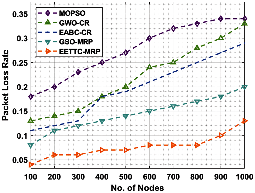
Figure 5: Packet loss rate analysis of EETTC-MRP algorithm

The results of NLT analysis for the presented EETTC-MRP technique in terms of FND, HND, and LND are shown in Tab. 5 and Fig. 6. The outcomes infer that the proposed EETTC-MRP technique gained the maximum NLT over other techniques. For instance, EETTC-MRP technique offered a lengthened FND of 2211 rounds, whereas MOPSO, GWO-CR, EABC-CR, and GSO-MRP techniques attained the least FND values such as 668, 963, 1301, and 1932 rounds respectively. Moreover, EETTC-MRP approach presented a lengthened HND of 6277 rounds, whereas MOPSO, GWO-CR, EABC-CR, and GSO-MRP methods reached less HND values such as 4199, 4623, 5237, and 5707 rounds correspondingly. Furthermore, the presented EETTC-MRP algorithm accomplished a lengthened LND of 9386 rounds, whereas MOPSO, GWO-CR, EABC-CR, and GSO-MRP methodologies achieved minimal LND values such as 6828, 7603, 8218, and 8412 rounds correspondingly. From the detailed results of the analysis, it has been established that the proposed EETTC-MRP technique is superior in terms of energy efficiency and NLT in IoT-assisted WSN.

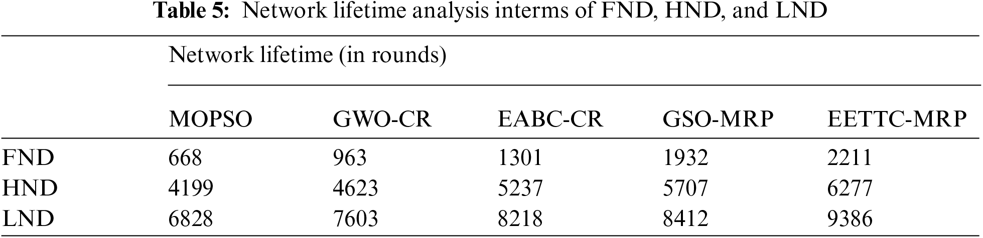
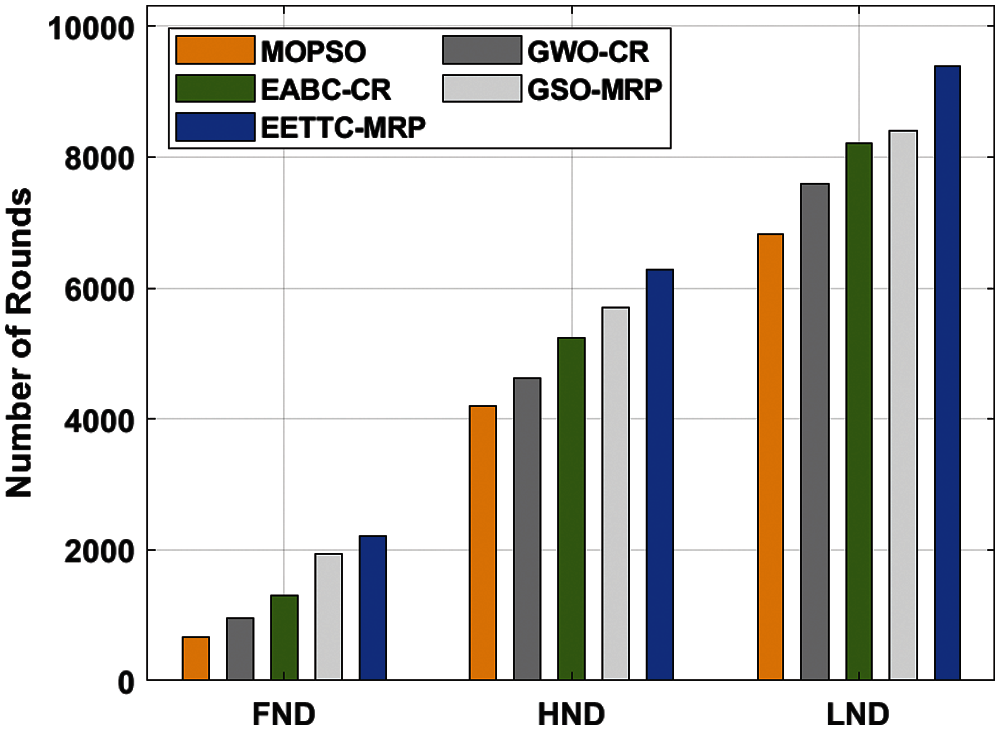
Figure 6: Network lifetime analysis of EETTC-MRP algorithm

4  Conclusion

In this study, a new EETTC-MRP technique is designed to achieve energy efficiency in IoT-assisted WSN. The proposed EETTC-MRP technique encompasses three major processes namely, T2FL-TCH, QGTOA-FCH, and PO-MHR. The use of T2FL for the selection of TCH helps in the appropriate selection of an optimal candidate CHs for final selection. In addition, the design of PO-MHR technique assists in deriving an optimal set of routes to BS, in such a way, to minimize energy consumption. A widespread experimental analysis was conducted and the outcomes were inspected under different evaluation parameters. The experimental results showcase the supremacy of EETTC-MRP technique over other techniques with a lengthened LND of 9386 rounds. In future, the performance of EETTC-MRP technique can be improved by including data aggregation design and MAC scheduling approaches.

Funding Statement: Shabnam Mohamed Aslam would like to thank the Deanship of Scientific Research at Majmaah University for supporting this work under Project No. R-2021-242.

Conflicts of Interest: The authors declare that they have no conflicts of interest to report regarding the present study.

This work is licensed under a Creative Commons Attribution 4.0 International License, which permits unrestricted use, distribution, and reproduction in any medium, provided the original work is properly cited.