Computers, Materials & Continua DOI:10.32604/cmc.2022.022692
Article

Modeling of Artificial Intelligence Based Traffic Flow Prediction with Weather Conditions

Mesfer Al Duhayyim1, Amani Abdulrahman Albraikan2, Fahd N. Al-Wesabi3,4, Hiba M. Burbur5, Mohammad Alamgeer6, Anwer Mustafa Hilal7, Manar Ahmed Hamza7,* and Mohammed Rizwanullah7

1Department of Natural and Applied Sciences, College of Community-Aflaj, Prince Sattam Bin Abdulaziz University, Al-Kharj, 16278, Saudi Arabia
2Department of Information Systems, College of Computer and Information Sciences, Princess Nourah Bint Abdulrahman University, Riyadh, 11564, Saudi Arabia
3Department of Computer Science, College of Science & Arts at Mahayil, King Khalid University, Muhayel Aseer, 62529, Saudi Arabia
4Faculty of Computer and IT, Sana'a University, Sana'a, 61101, Yemen
5Department of Computer Science, College of Science and Arts in Al-Bukairiyah, Qassim University, Al-Bukairiyah, 52571, Saudi Arabia
6Department of Information Systems, College of Science & Arts at Mahayil, King Khalid University, Muhayel Aseer, 62529, Saudi Arabia
7Department of Computer and Self Development, Preparatory Year Deanship, Prince Sattam Bin Abdulaziz University, Al-Kharj, 16278, Saudi Arabia
*Corresponding Author: Manar Ahmed Hamza. Email: ma.hamza@psau.edu.sa
Received: 16 August 2021; Accepted: 16 September 2021

Abstract: Short-term traffic flow prediction (TFP) is an important area in intelligent transportation system (ITS), which is used to reduce traffic congestion. But the avail of traffic flow data with temporal features and periodic features are susceptible to weather conditions, making TFP a challenging issue. TFP process are significantly influenced by several factors like accident and weather. Particularly, the inclement weather conditions may have an extreme impact on travel time and traffic flow. Since most of the existing TFP techniques do not consider the impact of weather conditions on the TF, it is needed to develop effective TFP with the consideration of extreme weather conditions. In this view, this paper designs an artificial intelligence based TFP with weather conditions (AITFP-WC) for smart cities. The goal of the AITFP-WC model is to enhance the performance of the TFP model with the inclusion of weather related conditions. The proposed AITFP-WC technique includes Elman neural network (ENN) model to predict the flow of traffic in smart cities. Besides, tunicate swarm algorithm with feed forward neural networks (TSA-FFNN) model is employed for the weather and periodicity analysis. At last, a fusion of TFP and WPA processes takes place using the FFNN model to determine the final prediction output. In order to assess the enhanced predictive outcome of the AITFP-WC model, an extensive simulation analysis is carried out. The experimental values highlighted the enhanced performance of the AITFP-WC technique over the recent state of art methods.

Keywords: Smart cities; artificial intelligence; urban transportation; deep learning; weather condition; TFP

1  Introduction

A survey reported that, in 2050, the global urban population is expected to attain 66% or 70% correspondingly. This upsurge in urbanization would have severe impact on cities’ management, security, and the environment. To effectively manage the meteoric growth in urbanization, several countries have projected the idea of smart cities to efficiently handle the resources and enhance energy utilization. The smart cities project could accurately handle the green environment by adopting and developing lower carbon emission techniques. Several countries (like Japan, US, EU, and so on.) all over the world have projected and realized the smart cities project for definitively accomplishing the future problems. For meeting the needs of a smart city, effective usage of information and communication technologies (ICTs) are essential [1] for sufficiently manage the data communications, data analyses, and efficient execution of complicated approaches for ensuring the secure and smooth operations of a smart city.

The IoT is the most significant and important component of the smart city applications that are accountable for producing large number of data [2]. In the existence of amount of complex and big data, it is complex to accurately determine the most effective and accurate performances. The optimum analyses of the big data could be executed by an innovative method such as Deep Reinforcement Learning (DRL), Artificial intelligence (AI), and Machine learning (ML), for reaching an optimum decision. The previous technique considers a long-term objective and could lead to an optimal or near optimum control decision [3]. The precision and accuracy of the above-mentioned methods could be enhanced further by increasing the number of training data to reinforce their learning abilities and thus the automatic decision efficacies. In [4], the researchers have displayed that the idea of smart cities realization and the utilization of innovative data analyses techniques for Big Data has increased nearly in the same years. The idea of IoT, smart cities, unmanned aerial vehicles (UAVs), Blockchain, and the utilization of DRL, AI, & ML based methods in several applications are yet in the evolution stage and eventually will provide better chances.

The growth of intelligent transportation systems (ITS) needs a higher degree of carrying capacity as an assurance [5]. Due to their high capacity and flexibility, vehicles are the main resources of transportation. Assuring traffic performance would have a significant effect on operation of the city. But, with the constant surge of vehicle ownership, the inadequate carrying capability of urban roads has slowed down the traffic performance of vehicles. Timely and accurate predictions of traffic flow (TF) give consistent basis of traffic control for governors and provide suitable travel guidance for the tourists thus enhancing road network and decrease traffic congestion [6]. But, traffic prediction is a nonlinear and sophisticated challenge. In reality, TF has clear periodicity and temporal correlation, however, it might develop in an irregular manner under the disturbance of weather modifications that creates this problem more complex. The present short-term TFP methods could be generally separated into three classifications: DL, statistical modules, and conventional ML methods.

Related to the statistical models, conventional ML approaches such as SVM and SVR shows powerful function fitting capability in nonlinear and complex TFP problem. The fundamental concept of this type of technique is to convert lower dimension and linearly inseparable traffic data to higher dimension and linearly separable expression via kernel function. With the development of traffic big data [7], short-term traffic prediction has to turn into more complex and challenging that propose higher needs for modelling data. DL modules, with the efficiency for higher dimension space modelling and the capability for extracting features of variables via hierarchical depiction, have turn into the popular technology of TFP. [8] proposed a short-term multistep freeway TFP method using RBF where center position of hidden layer is established by the fuzzy c-means clustering. [9] initially utilized SAE for learning the depiction of TF features for predicting.

This paper introduces a novel artificial intelligence (AI) based TFP with weather conditions (AITFP-WC) for smart cities. The AITFP-WC model focuses on the improvement of the predictive performance of the TF with the consideration of weather related conditions. The proposed AITFP-WC technique involves Elman neural network (ENN) model for TFP in smart cities. In addition, tunicate swarm algorithm with feed forward neural networks (TSA-FFNN) model is utilized for the weather and periodicity analysis. Furthermore, a fusion of TFP and WPA processes takes place using the FFNN model to determine the final prediction output. For examining the increased prediction performance of the AITFP-WC model, a series of experiments were carried out on TF and weather data.

2  Existing Traffic Flow Prediction Models

Lu et al. [10], proposed an integrated predictive technique for short term TF that relies on LSTM-NN and ARIMA. This technique can create short-term predictions of upcoming TF depends on the past traffic data. Initially, the LR feature of traffic data was taken by the rolling regression ARIMA module; later, BP was utilized for training the LSTM network to take nonlinear features of traffic data; and lastly, relies on the dynamic weighting of sliding window integrated the predictive influences of this 2 methods. Kong et al. [11] take RBM as the technique for predicting TF that is a usual process relies on DL framework. RBM creates the long-term module of polymorphic for chaotic time sequence, with phase space recreation for recognizing the data.

Hou et al. [12] proposed an integrated structure of SAE and RBF NN for predicting TF that could efficiently capture the disturbance of weather factors and periodicity of TF and data temporal correlation. Initially, SAE is utilized for processing the TF data in many time slices for acquiring early predictions. Later, RBF is utilized for capturing the relation among periodicity of TF and weather disturbance thus gaining other predictions. Lastly, alternative RBF is utilized for combining the above 2 predictions on decision level, obtain a recreated prediction with high precision.

Zheng et al. [13] focused on the short term TF predictive problems on the basis of real time traffic data as one crucial module of a smart cities. In contradiction of long term traffic prediction, precise prediction of short term TF facilitate rapid response and timely traffic management. They developed and studied a new EM on the basis of LSTM, DAE, and CNN modules. This method considered spatial & temporal features of the traffic condition. In Rajendran et al. [14], the structural patterns of TF could be pinched from freeway toll data accordingly, a novel predictive module has been projected. Locally weighted learning is utilized for predicting the subsequent sample TF of current sector and the succeeding station entrance flow. This learning module places nonlinear and linear modules for fitting the adjacent points and later employs this value for predicting query point values.

Kang et al. [15], proposed a hybrid module for spatio temporal feature extraction and prediction of urban road network travel time that integrates EDM and CN with an XGBoost predictive module. Because of the dynamic nature and high nonlinear travel time sequence, it is essential for considering time reliance and spatial dependence of travel time sequence to predict the travel time of road network. The dynamic feature of travel time sequence could be exposed through the EDM technique, a non-linear technique is depending upon Chaos concept. In Raza et al. [16], GA is utilized for designing ANN and LWR modules. This proposed method is based on the integration of GA, NN, and LWR for achieving optimum predictive efficiency in several traffic and input conditions. The GA aimed ANN (GA-ANN) and GA aimed LWR (GA-LWR) disaggregate and aggregate modules are utilized for predicting short term traffic (five minutes) for 4 lanes of urban road in Beijing, China.

3  Problem Statement and Data Used

This section offers the detailed problem statement of this study and also explained the data (including traffic and weather data) employed for validation.

3.1 Problem Statement

TFP model makes use of existing traffic and weather-related parameters to estimate the output flow in any succeeding time slices. The outcome y of the predictive technique is defined using Eq. (1):

y=f(X1,X2,X3,…,X10,X11,X12).(1)

It is considered that the TF data is not limited only to the regularity and again affected by other weather conditions, the input variables of the model want to comprise external weather conditions. Here, Xi denotes the dataset on the time slice i, counting flow xiflow, time expression xitimecode, vector depiction of embedding xembedding, and weather variables xiweathercondition; Xi is defined by

Xi=[xflow,xtimecode,xembedding,xweathercondition],(2)

where yflow signifies the flow prediction depending upon the traffic series data and yweather&time signifies the flow prediction depending upon the weather as well as time periodicity [17]. By the view of decision level data fusion, the end flow prediction value is the fusion value of two decisions, therefore the outcome y of the integrated model can be defined using Eq. (3):

y=ffusion(yflow,yweather\&time).(3)

For multistep prediction, y can be defined as yi, and i indicates the step size.

3.2 Traffic and Weather Data

The traffic dataset of metro freeway in the Twin Cities is used [17]. The actual dataset is gathered at a 30 s duration of at least 4,500 loop detectors. During the preprocessing level, the data gets preprocessed in the form of table with 5 mts duration. In addition, time similarity measure is used to correct the errors and omissions. For revealing the periodicity of traffic data under weather disturbances, a time-flow correlation is derived. Besides, the training data gets partitioned into working and non-working days, and the average flow in each time slice is calculated. The time flow correlation for the time slices can be represented in Eq. (4):

xttimecode=1n∑j=0n⁡xi,jflow,(4)

where xi,jflow signifies the flow of time slice i on day j.

Next, the weather dataset [17] is collected and used 1-hot coding technique to handle the non-numerical parameters. Besides, an embedding element is employed for extracting the expression of high dimensional data of weather type. In addition, the embedding vector of weather type is represented using Eq. (5):

xembedding=fembedding(xone-hot),(5)

where xembedding denotes the trained embedded vector of weather types, whereas xone represents 1-hot expression. For variable selection related to TF, Pearson correlation coefficient ρ is determined using Eq. (6) is calculated, where X and Y denotes a set of 2 target parameters.

ρX,Y=cov(X,Y)σXσY=E[(X−μX)(Y−μY)]σXσY.(6)

To extract the additional weather variables, the PCA technique can be employed for the data fusion process at the feature level. The actual matrix A of weather variables can be denoted as follows:

A=(x1DBx1RHx1Visx1WBx1WSx2DBx2RHx2Visx2WBx2WS⋯⋯⋯⋯⋯xn−1DBxn−1RHxn−1Visxn−1WBxn−1WSxnDBxnRHxnVisxnWBxnWS),(7)

where xDB, xRH, xVis, xWB, and xWS are the designated variables. Once the PCA is employed, the resultant matrix Pcan be produced as shown below.

P=fPCA(A)=(x1pcax2pca⋯xn−1pcaxnpca),(8)

where xpca is the fusion value of the elected weather variables examined by PCA.

4  The Proposed Model

The overall framework of the proposed AITFP-WC technique encompasses three major levels namely ENN based TFP, TSA-FFNN based WSA, and fusion process. Fig. 1 demonstrates the overall process of TFP process. The detailed working of every level is offered in the next subsections.

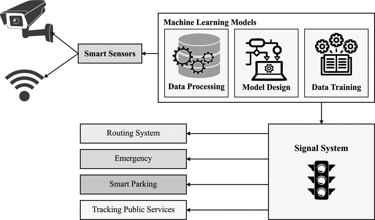
Figure 1: Systematic framework of TFP in smart cities

4.1 Level I: TFP

At the first level, the AITFP-WC technique exploits the ENN model to forecast TF. The ENN model is employed for the extraction of temporal correlation exist in the TF. Fig. 2 shows a simple structure of an ENN. The ENN model comprises four major layers namely input, context, hidden, and output layers. The major configuration of the ENN model is similar to the FFNN in such a way that the connections except context layer are identical to MLP. The context layer receives the input from the output of the hidden layer to store the earlier values of the hidden layer. The external input, context weight, and output weight matrices can be represented as Whi,Whc,Wh0, respectively. The dimensions of the input and output layers are n, i.e., x1(t)=[x11(t),x21(t),…,xn1(t)]T, y(t)=[y1(t),y2(t),…,yn(t)]T and the dimension of the context layer is m.

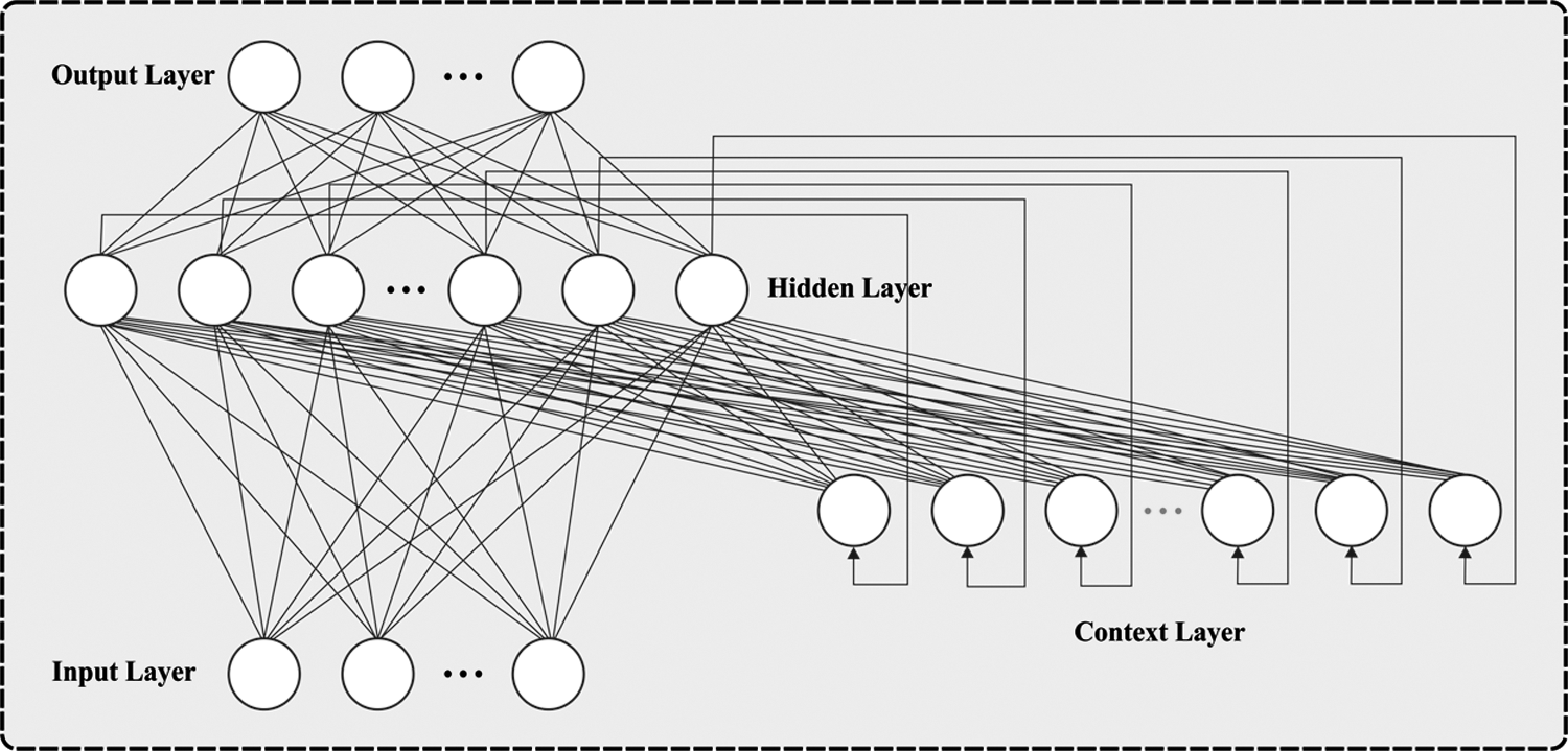
Figure 2: Structure of ENN

The input layer of the ENN model is defined in Eq. (9):

ui(l)=ei(l),i=1,2,…,n(9)

where l demonstrates the input and the output layers in round l. Afterward, the kth hidden layer in the network can be represented using Eq. (10):

vk(l)=∑j=1Nωkj1(l)xjc(l)+∑i=1nωki2(l)ui(l)k=1,2,…,N(10)

where, xjc(l) defines the signal which is passed from the kth context layer node, ωkj1(l) designates the ith and jth weights of the hidden layers directed from othnode [18]. At last, the outcome of the hidden layer can be fed into the context layer is given below:

Wk(l)=f0(v¯k(l))(11)

where,

v¯k(l)=vk(l)max{vk(l)}(12)

represents the normalized value of the hidden layer.

The following layer is the context layer, which can be defined as follows.

Ck(l)=βC,(l−1)+Wk(l−1),k=1,2,…,N(13)

where, Wk pointed out the gain of self linked feedback among 0 and 1. Lastly, the output layer at the network can be represented below.

y0(l)=∑k=1N⁡ωok3(l)Wk,(l),0=1,2,…,n(14)

where, ωok3 defines the weights of the connections from the kth layer into the oth layer.

4.2 Level II: Weather and Periodicity Analysis

In the second level, the WPA is performed using the TSA-FFNN technique, which makes use of processed variables comprising xembedding, xtimecode, and xpca, therefore, the TSA-FFNN function is denoted as follows.

yweather&time=fRBF(xembedding,xtimecode,xpca).(15)

The FFNN is an easier type of ANN that includes many processing modules called “neurons”. In FFNN, the data takes stimulated in single way, forwards from the input to output through hidden layer. It doesn't comprise some loop or cycle [19]. All individual neurons define the entire input weight and approved the sum through activation functions and so the result is obtained. It can be determined as Eqs. (16) and (17):

hj=∑i=lR⁡iwj,ixj+hbj,(16)

where iwj,i represents the weights related amongst the weight neurons i=(1,2,…,R) and j=(1,2,…,N), hbj implies the bias in hidden layers, R indicates the neuron count in the input layers, and xj denotes the respective input data. During this case, the S shaped curved sigmoid functions are utilized as activation functions as determined in Eq. (17):

f(x)=11+e−x.(17)

Therefore, the result of neurons in the hidden layers are determined as:

hoj=fj(hj)=1(1+e−hj).(18)

In the final layer, the result of neurons are signified as:

yk=fk(∑j=1N⁡hwk,jhoj+obk),(19)

where hwj,i refers the weights interconnected amongst neurons j=(1,2,…,N) and k=(1,2,…,S), obk stands for bias in final layer, N refers the neuron quantity in hidden layers, and S defines the neuron quantity in hidden layers. Usually, the training technique is carried out for modifying the weight and bias values till the maximal classification accuracy was gained.

In order to effectually adjust the parameters involved in the FFNN model, the TSA is employed. The motivation and scientific modeling of presented TSA technique are explained in detail. Tunicate has capability for finding the place of feed source in sea. But there is no knowledge about the feed source in the provided search space. In TSA, 2 performances of tunicates are utilized to determine the feed source and they are jet propulsion and SI. In order to scientifically process the jet propulsion performance, the tunicate can fulfill 3 situations such as avoid the fights amongst searching agents, movement near the place of optimum searching agents, and remained nearby the optimum searching agents. While the swarm performance upgrades the places of another search agent on the optimum solution [20]. The mathematical process of the performance is explained in the following.

For avoiding the fights amongst searching agents (for instance, another tunicate), vector A→ is utilized for the computation of novel search agent place as given below.

A→=G→M→(20)

G→=c2+c3−F→(21)

F→=2⋅c1(22)

But G→ implies the grariab less and F→ depicts the water flow advection in deep ocean. The variables c1,c2, and c3 are arbitrary numbers lies in [0,1], M→ stands for the social force amongst searching agents. The vector M→ was computed as:

M→=⌊Pmin+c1⋅Pmax−Pmin⌋(23)

where Pmin and Pmax signifies the primary and subordinate speeds for making social interface. In this work, of values of Pmin and Pmax are considered as 1 and 4, correspondingly.

Afterward, in order to avoid the fight amongst neighboring ones, the searching agents are travel near the direction of optimum neighbor.

P→D=|F→S−rand⋅P→p(x)|(24)

where P→D implies the distance amongst the feed source and search feed, for instance, tunicate, x denotes the present iterations, F→S stands for the place of feed source, for sample, optimal. The vector P→p(x) represents the place of tunicate and rand signifies the arbitrary number in range 0 and 1.The searching agents are continuing their place near the optimum search agent (for instance, feed source).

P→p(x)={F→S+A→⋅P→Difrand≥0.5F→S−A→⋅P→Difrand<0.5(25)

where P→p(x′) represents the upgraded place of tunicate interms of place of feed source F→S.

For mathematically simulating the swarm performance of tunicate, initial 2 optimum solutions are stored and upgraded the places of other searching agents based on the place of an optimum search agent. The subsequent equation is presented for defining the swarm performance of tunicate:

Pp(x+1)=Pp(x)+Pp(x+1)2+c1(26)

The steps and flowchart presented are provided under.

i. Initialization of the tunicate population P→.

ii. Select the primary variables and maximal iteration count.

iii. Compute the fitness value of all searching agents.

iv. Afterward calculating the fitness value, the optimum searching agent is traveled in provided searching area.

v. Upgrade the place of all searching agents utilizing Eq. (26).

vi. Alter the upgraded searching agent that drives away from the boundary in provided search space.

vii. Calculate the upgraded searching agent fitness values. When there is an optimum solution compared to the preceding optimum solution, next upgrade Pp.

viii. When the termination condition is fulfilled, next the TSA gets stopped. Then, repeat Steps 5–8.

ix. Obtain optimum solutions.

4.3 Level III: Decision Level Data Fusion Model

The data fusion process takes place using FFNN model which aims to tune the features outcomes offered from the previous two modules. Since FFNN is a type of NN with easier architecture, it is not required to treat the hierarchical structure during modeling, and it could satisfy the need for data fusion in features as well as decision levels. The outcome of the fusion model is the end predictive results of the AITFP-WC model and it can be represented as follows.

y=yfusion=ffusion(yflow,yweather&time).(27)

5  Results and Discussion

This section validates the TFP performance of the AITFP-WC technique over other existing techniques. Tab. 1 and Fig. 3 demonstrates the results analysis of the AITFP-WC technique with other techniques on weather data. From the obtained results, it is evident that the AITFP-WC technique has attained improved predictive outcomes on the weather data. The experimental results ensured that the AITFP-WC technique has outperformed the existing techniques with the MAPE of 17.326%, MSE of 313.417, and RMSE of 17.704. At the same time, the least performance is obtained by the RBF+PCC+PCA+BP with the MAPE of 21.446%, MSE of 517.261, and RMSE of 22.743.

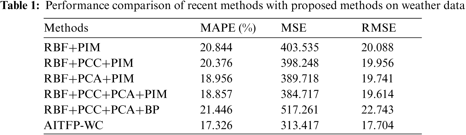
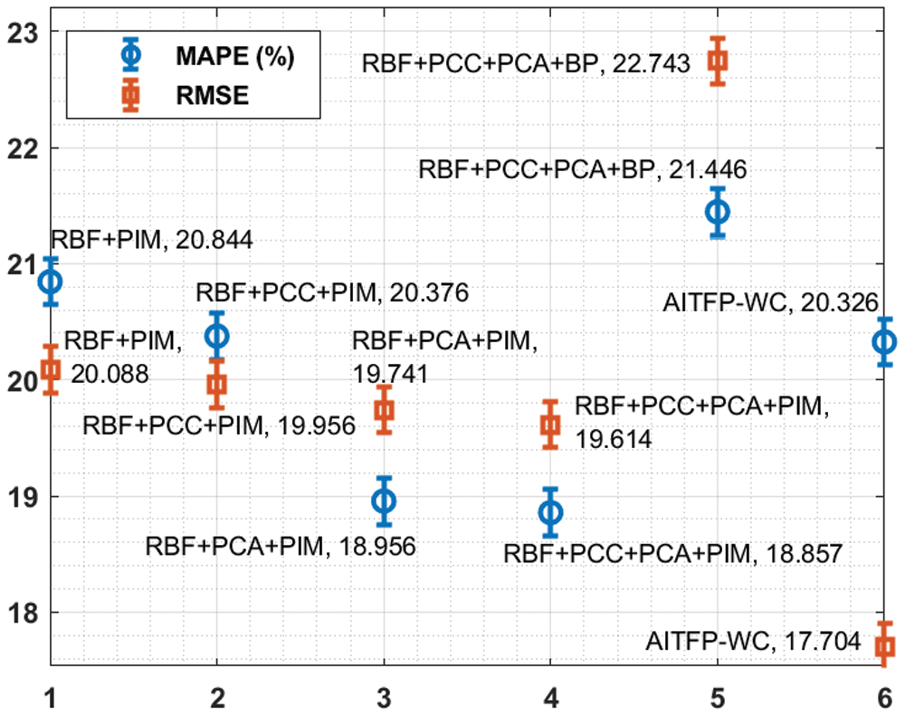
Figure 3: MAPE and RMSE analysis of AITFP-WC technique on weather data

Another comparison study of the AITFP-WC technique with baseline techniques is made in Tab. 2 and Fig. 4. From the obtained values, it is evident that the LSTM and GRU techniques have showcased inferior outcomes with the maximum MAPE of 11.341% and 11.896%. Followed by, the S.LSTM, S.GRU, SAE, and Fusion-ANN models have demonstrated moderate MAPE of 10.574%, 10.628%, 10.558%, and 10.537% respectively. In line with, the SAERBF technique has exhibited near optimal performance with the MAPE of 10.378%. However, the proposed AITFP-WC technique has demonstrated superior outcomes with the minimal MAPE of 10.280%.

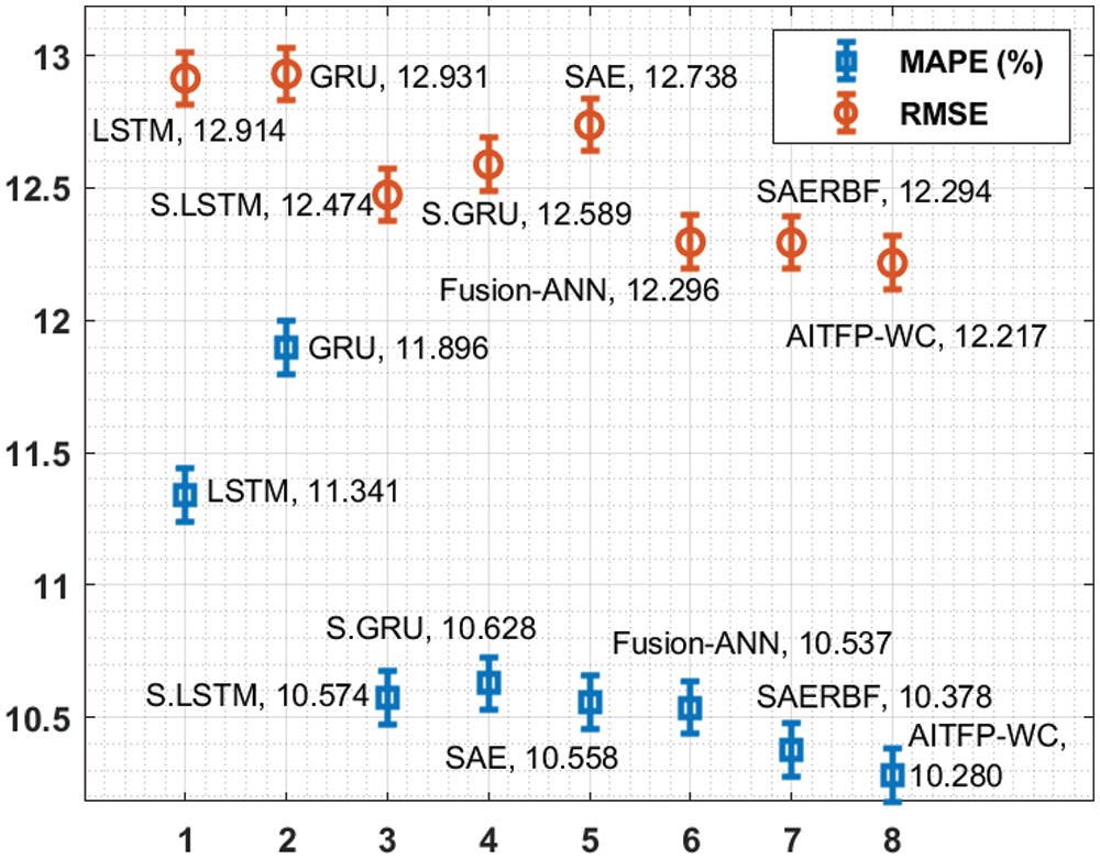
Figure 4: Comparative MAPE and RMSE analysis of AITFP-WC technique with existing methods

A brief TFP predictive performance of the AITFP-WC technique interms of MAPE take place in Tab. 3 and Fig. 5. The experimental results depicted that the AITFP-WC technique has offered effectual TFP outcomes under varying time intervals. For instance, with 5 min interval, the AITFP-WC technique has attained a lower MAPE of 10.28% whereas the LSTM, GRU, S.LSTM, S.GRU, SAE, FUSION-ANN, and SAERBF techniques have depicted a higher MAPE of 11.34%, 11.89%, 10.57%, 10.62%, 10.55%, 10.53%, and 10.37% respectively. Eventually, with 15 min interval, the AITFP-WC approach has attained a lesser MAPE of 12.64% whereas the LSTM, GRU, S.LSTM, S.GRU, SAE, FUSION-ANN, and SAERBF manners have showcased a higher MAPE of 15.07%, 15.29%, 13.92%, 13.75%, 13.82%, 13.26%, and 12.92% respectively. Meanwhile, with 30 min interval, the AITFP-WC technique has attained a minimum MAPE of 16.12% whereas the LSTM, GRU, S.LSTM, S.GRU, SAE, FUSION-ANN, and SAERBF algorithms have depicted a superior MAPE of 19.75%, 19.62%, 17.93%, 17.64%, 17.85%, 16.20% and 16.12% correspondingly.

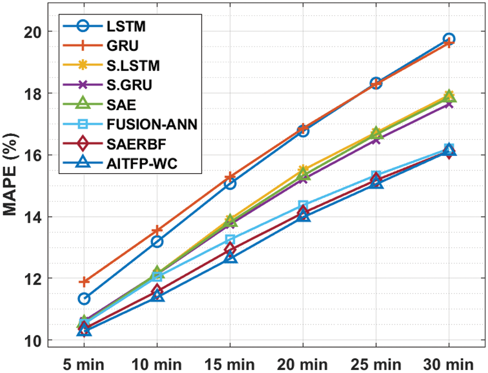
Figure 5: MAPE analysis of AITFP-WC model with existing techniques

A detailed TFP predictive performance of the AITFP-WC technique with respect to MSE takes place in Tab. 4 and Fig. 6. The experimental outcomes showcased that the AITFP-WC approach has offered effective TFP outcomes under varying time intervals. For instance, with 5 min interval, the AITFP-WC manner has gained the least MSE of 149.25% whereas the LSTM, GRU, S.LSTM, S.GRU, SAE, FUSION-ANN, and SAERBF techniques have depicted a higher MSE of 166.77%, 167.20%, 155.60%, 158.47%, 162.25%, 151.19%, and 151.15% respectively. Also, with 15 min interval, the AITFP-WC technique has attained a lower MSE of 207.48% whereas the LSTM, GRU, S.LSTM, S.GRU, SAE, FUSION-ANN, and SAERBF methodologies have exhibited a higher MSE of 264.90%, 263.18%, 234.77%, 236.78%, 258.00%, 213.09%, and 211.28% respectively. In the meantime, with 30 min interval, the AITFP-WC technique has attained a lower MSE of 328.43% whereas the LSTM, GRU, S.LSTM, S.GRU, SAE, FUSION-ANN, and SAERBF methods have outperformed a higher MSE of 434.19%, 434.89%, 370.32%, 369.00%, 441.44%, 326.71%, and 331.33% respectively.

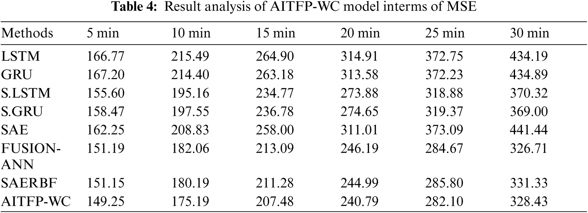
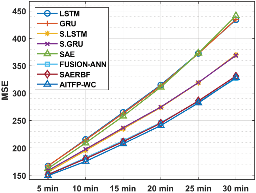
Figure 6: MSE analysis of AITFP-WC model with existing techniques

A brief TFP predictive performance of the AITFP-WC method interms of RMSE take place in Tab. 5 and Fig. 7. The experimental results outperformed that the AITFP-WC algorithm has offered effectual TFP outcomes under varying time intervals. For instance, with 5 min interval, the AITFP-WC method has attained a minimum RMSE of 12.22% whereas the LSTM, GRU, S.LSTM, S.GRU, SAE, FUSION-ANN, and SAERBF techniques have depicted a maximal RMSE of 12.91%, 12.93%, 12.47%, 12.59%, 12.74%, 12.30% and 12.29% correspondingly. Besides, with 15 min interval, the AITFP-WC approach has attained a lower RMSE of 14.40% whereas the LSTM, GRU, S.LSTM, S.GRU, SAE, FUSION-ANN, and SAERBF techniques have depicted a superior RMSE of 16.28%, 16.22%, 15.32%, 15.39%, 16.06%, 14.60% and 14.54% correspondingly. Likewise, with 30 min interval, the AITFP-WC manner has gained a lower RMSE of 18.12% whereas the LSTM, GRU, S.LSTM, S.GRU, SAE, FUSION-ANN, and SAERBF techniques have demonstrated a maximum RMSE of 20.84%, 20.85%, 19.24%, 19.21%, 21.01%, 18.08% and 18.12% correspondingly.

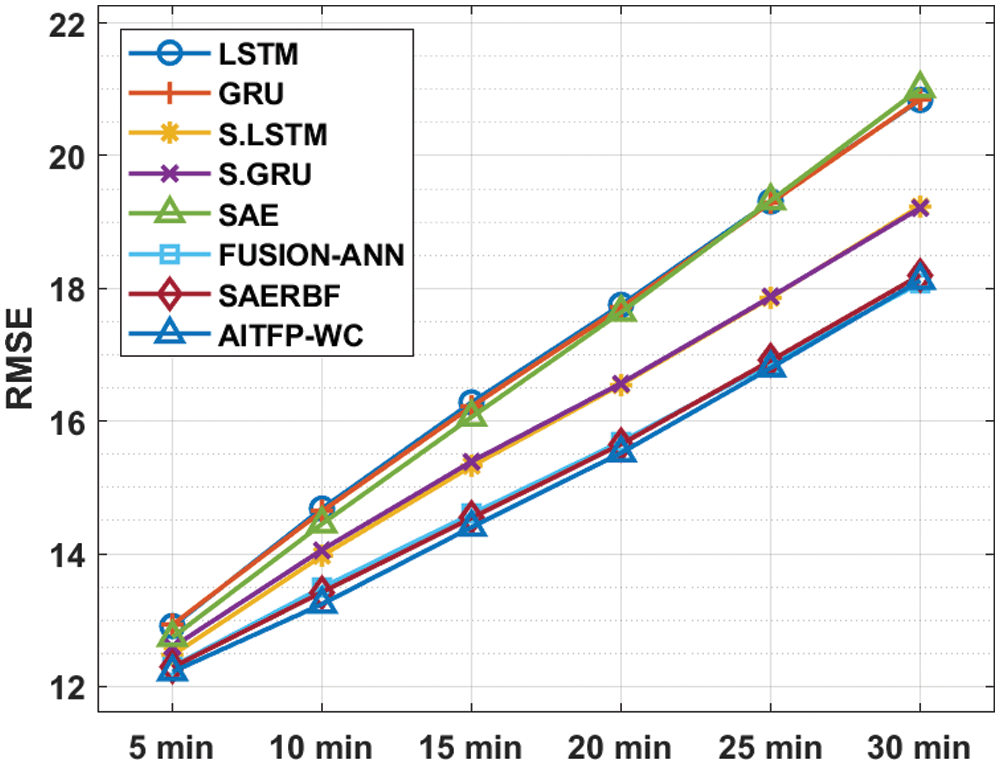
Figure 7: RMSE analysis of AITFP-WC model with existing techniques

6  Conclusion

In this study, a new AITFP-WC technique is designed to predict the flow of traffic with weather conditions in smart cities. The proposed AITFP-WC technique encompasses ENN based TFP, TSA-FFNN based WSA, and FFNN based data fusion processes. In TSA-FFNN model, the TSA is used to optimally tune the parameters involved in the FFNN model and thereby raises the predictive performance to a maximum extent. For examining the increased prediction performance of the AITFP-WC model, a series of experiments were carried out on TF and weather data. The experimental values pointed out the supremacy of the AITFP-WC technique over the recent state of art methods. Therefore, the AITFP-WC technique can be used in real time smart city environment to predict the flow of traffic under extreme weather conditions. In future scope, the efficacy of the AITFP-WC technique can be boosted by the use of advanced DL architectures with learning rate scheduling approaches.

Funding Statement: The authors extend their appreciation to the Deanship of Scientific Research at King Khalid University for funding this work under grant number (RGP1/53/42), https://www.kku.edu.sa. This research was funded by the Deanship of Scientific Research at Princess Nourah bint Abdulrahman University through the Fast-track Research Funding Program.

Conflicts of Interest: The authors declare that they have no conflicts of interest to report regarding the present study.

This work is licensed under a Creative Commons Attribution 4.0 International License, which permits unrestricted use, distribution, and reproduction in any medium, provided the original work is properly cited.