DOI:10.32604/cmc.2022.022726
| Computers, Materials & Continua DOI:10.32604/cmc.2022.022726 | |
| Article |
Optimizing Steering Angle Predictive Convolutional Neural Network for Autonomous Car
1Control, Automotive and Robotics Lab Affiliated lab of National Center of Robotics and Automation (NCRA HEC Pakistan), and with the Department of Computer Science and Information Technology, Mirpur University of Science and Technology (MUST), Mirpur Azad Kashmir, 10250, Pakistan
2College of Computer Science and Information System, Najran University, Najran, 61441, Saudi Arabia
3College of Computer Science and Engineering, University of South Florida, Tampa, 33620, United States
*Corresponding Author: Adel Rajab. Email: 77adel.rajab@gmail.com
Received: 17 August 2021; Accepted: 29 September 2021
Abstract: Deep learning techniques, particularly convolutional neural networks (CNNs), have exhibited remarkable performance in solving vision-related problems, especially in unpredictable, dynamic, and challenging environments. In autonomous vehicles, imitation-learning-based steering angle prediction is viable due to the visual imagery comprehension of CNNs. In this regard, globally, researchers are currently focusing on the architectural design and optimization of the hyperparameters of CNNs to achieve the best results. Literature has proven the superiority of metaheuristic algorithms over the manual-tuning of CNNs. However, to the best of our knowledge, these techniques are yet to be applied to address the problem of imitation-learning-based steering angle prediction. Thus, in this study, we examine the application of the bat algorithm and particle swarm optimization algorithm for the optimization of the CNN model and its hyperparameters, which are employed to solve the steering angle prediction problem. To validate the performance of each hyperparameters’ set and architectural parameters’ set, we utilized the Udacity steering angle dataset and obtained the best results at the following hyperparameter set: optimizer, Adagrad; learning rate, 0.0052; and nonlinear activation function, exponential linear unit. As per our findings, we determined that the deep learning models show better results but require more training epochs and time as compared to shallower ones. Results show the superiority of our approach in optimizing CNNs through metaheuristic algorithms as compared with the manual-tuning approach. Infield testing was also performed using the model trained with the optimal architecture, which we developed using our approach.
Keywords: Bat algorithm; convolutional neural network; hyperparameters; metaheuristic optimization algorithm; steering angle prediction
In recent years, we have witnessed a storm of advancements in autonomous self-driving ground vehicles, and significant research efforts in the industry and academia are being devoted to their successful implementation. In this regard, one of the challenges identified is the accurate prediction of the steering angle required for a vehicle to autonomously steer on a given terrain, due to the heterogeneity of roads and their geometries. A recent solution has been proposed to address these challenges in steering angle prediction, that is, by learning from demonstration, also known as imitation learning [1].
In autonomous vehicles, imitation learning is used to learn the steering angle to drive in different scenarios through human driving demonstration. For this purpose, corresponding steering angles are collected simultaneously while driving the vehicle, and these are used as training data for the supervised learning by an artificial neural network (ANN) model. That is, the steering angle is predicted by the ANN model using raw image pixels as the input [2–4]. Once the model learns, it can then autonomously predict steering angles without human intervention. For this type of supervised learning steering angle prediction problem, the convolutional neural network (CNN) and its variants are mostly employed due to their remarkable performance in visual imagery understanding [5]. However, the performance of these networks strongly depends on their architecture, design, and training parameters [6].
The process of designing the architecture of an ANN and tuning the hyperparameters to achieve optimal results for a particular problem has been identified to be strenuous and remains to be under investigation by researchers globally [7]. This becomes even more challenging when the dimensionality of the hyperparameter space increases. In particular, deep neural networks have different hyperparameters that need to be adjusted given any input dataset, giving rise to high-dimensional search space. The primary hyperparameters of the CNN that contribute to the accuracy of results and speed of convergence include the learning rate, optimizer function, number of epochs, batch size, activation function, dropout rate, number and sequence of layers (convolutional (Conv), pooling, and fully connected (FC) layers), number of neurons in the FC layers, and number and size of the filters in each Conv layer. Each setting, having a specific combination of all these hyperparameters, has a different impact on the performance of the neural network. The process of tuning all these hyperparameters and evaluating the results for each setting is tedious, time-consuming, and computationally expensive [8].
Literature has proven the competence of many nature-inspired metaheuristic algorithms, including the genetic algorithm [9–12], swarm intelligence optimization algorithms [13–18], and their variants, for the optimization of hyperparameters. The optimization of the hyperparameters of a steering angle predictive neural network has been determined to be a nonlinear, non-convex, and complex global optimization problem. To solve this kind of problem, the bat algorithm and its variants have shown efficient results as compared to other metaheuristic algorithms in the previous studies [19–21]. On these grounds, the prospect of the bat algorithm for tuning the CNN can be envisaged. However, the algorithm has never been used in tuning the hyperparameters of CNN. Moreover, for the steering angle prediction, various architectures of neural networks have been proposed by researchers; most of them have manually modified the hyperparameters of CNN to determine the combination(s) of values that afford the best results [22,23]. However, no research has been conducted on the utilization of metaheuristic algorithms for the optimization of steering angle predictive CNN. This motivated us to explore the application of two metaheuristic algorithms in realizing optimal steering angle predictive CNNs. Our research is divided into two steps. In the first step, we optimize the learning rate, batch size, activation function, and optimizer using the bat algorithm. In the second step, one of the optimal settings of these hyperparameters is selected to optimize five architectural units of CNN using the bat algorithm, namely, the number of Conv layers, number of filters in each Conv layer, size of each filter, number of FC layers, and number of neurons in each FC layer. Moreover, these five architectural parameters are also optimized using the basic Particle Swarm Optimization (PSO) algorithm. This is performed to determine the effectiveness of the bat algorithm in solving the problem under discussion by comparing the results of the bat algorithm and the PSO algorithm. For this purpose, the same number of generations, population size, and encoding scheme of the CNN architecture is used. During whole process of optimization in our methodology, we adapted early stopping, which involves stopping the training after some epochs if the model failed to improve. Finally, the optimal CNN model architecture is trained with more data and used in infield experiments.
The main contributions of this study are as follows:
• Deploying bat and PSO algorithms for the automatic tuning of nine major architectural and training parameters of CNN, including the number of Conv layers, number of filters in each Conv layer, number of fully connected layers, number of nodes in the FC layers, batch size, dropout rate, activation function, optimizer, and learning rate.
• Providing CNN model architectures and hyperparameters with improved results for the steering angle prediction problem.
• Employing Udacity dataset in evaluating the performance of the metaheuristic-based optimization approach.
• Validation of the results through infield testing of our developed prototype.
The rest of the paper is structured as follows: Section 2 outlines the literature review regarding the steering angle prediction and metaheuristic optimization algorithm. Section 3 gives a brief overview of the architecture, properties, and hyperparameters of the CNN. The standard bat algorithm is discussed in Section 4. In Section 5, a short introduction to the PSO algorithm is provided. The methodology of implementing the bat algorithm and the PSO algorithm for the CNN architectural units and other hyperparameter selections is elucidated in Section 6. Experiments and results are discussed in Section 7. Lastly, Section 8 concludes our research.
The study of steering angle prediction based on imitation learning began with the second Udacity competition related to the self-driving car. The winner of the competition developed 9-layered CNN, which was determined to be successful in autonomously driving the vehicle in the Udacity simulator. Since then, continuous research has been carried out on designing the optimal neural network architecture for steering angle prediction and finding hyperparameters that provide the best training results. Among these neural networks, the most commonly used architecture found in the literature is CNN.
Lately, many architectures of CNN have been proposed by researchers for steering angle prediction [24–29]. By analysis of available literature regarding the imitation-learning-based steering angle prediction, it was observed that the performance of a neural network architecture proposed in one research cannot be compared with an architecture proposed in another research. This is because the training and testing datasets used in each research is different. This persists even with the studies in which the same publicly available datasets were used. This is because has not been divided into training and testing sets by the publisher, so the train-test-split is different in different studies. Moreover, the evaluation metrics used in these studies vary from each other. Hence, there is an ambiguity in deciding which architecture of CNN and its hyperparameters should be used for training to utilize CNN for infield autonomous vehicles.
Recently, Kebria et al. [30] manually tuned 96 CNN models and equally trained on a subset of the Udacity dataset to explore and evaluated the impact of three architectural parameters of CNN, including the number of layers, number of filters in each layer, and the filter size on the performance of CNN for steering angle prediction. For this purpose, they incrementally increased the number of layers from 3 to 18, the number of filters from 4 to 128, and the filter sizes from 3 × 3 to 7 × 7, for designing CNN models. However, they did not perform infield testing to evaluate the performance of the best performing CNN model architecture obtained after the hand-tuning of architectures. Moreover, tuning CNN using a metaheuristic approach has proven its competence as compared to manually tuning it [31]. Jaddi et al. [32] have used a bat algorithm to optimize the architecture, as well as the weights and biases of simple feedforward neural networks. They tested the effectiveness of their approach using two-time series and six classification benchmark datasets. However, the process of tuning CNN is quite complex and challenging due to its disparate layers and dimensionality issues.
3 Convolutional Neural Network
In recent years, it has been established that CNNs can generate rich input image representations by embedding input images in fixed-length vectors, which can be used for a variety of visual tasks. However, CNN performance depends on datasets, architecture, and other training attributes [33,34]. The basic architecture of a CNN comprises input and output layers, as well as multiple hidden layers. CNN's hidden layer consists of a series of convolutional layers (Conv layer), a pooling layer, normalization layer(s), flatten layer, and fully connected layer(s). Central to the CNN are the Convolutional layers (Conv layer), in which filters convolve over the image and perform dot product with the image pixels. This operation is very important for indexes in a matrix as it affects how weights are determined at a particular index point. The output array obtained as a result of convolution is called a feature map. The number of feature maps yielded by a Conv layer equals the number of filters used in the layer. The number of parameters and output volume of a layer depends on the input size, filter size, number of filters, padding, and stride of filters. It is a convention to apply the activation layer immediately after each convolution layer. The objective of this layer is to incorporate nonlinearity into a system. Some commonly used nonlinear activation functions include Rectified Linear units (Relu), Leaky Relu, parametrized Relu, Elu, Selu, Sigmoid, Softmax, and Tanh. Where softmax and sigmoid are common to the output layer for the classification problem.
The batch size, learning rate, number of epochs, and optimizer are among the crucial training parameters influencing the performance of a CNN architecture being trained on a given dataset, where one epoch indicates that the entire dataset has traversed forward and backward through the CNN once. The batch size is the total number of training examples present in a single batch when the whole dataset is divided into batches. The learning rate governs the step size at each iteration while moving toward a minimum of a loss function. The optimizer is responsible for altering the weights inside the CNN. The commonly used optimizers for CNN are the stochastic gradient descent (Sgd), Adam, Adagrad, Nesterov accelerated gradient (NAG), AdaDelta, and RMSProp.
For training the ANN to perform steering angle prediction, the corresponding steering angles and images are collected while a car is being driven by a human driver. For this purpose, three methods are being used. In the first method, simulation software (such as CARSIM, CARLA, and TORCS) [35,36], is being used to generate the data sets required for this task. In the second method, images and corresponding steering angles are collected by a human-driven vehicle using onboard cameras and angle sensors [37,38]. Lastly, the third method involves utilizing the benchmark publicly available datasets (such as Udacity, DIPLECS, and Comma.ai) [39], for training ANNs to perform autonomous steering angle prediction.
Bat algorithm is a metaheuristic optimization algorithm proposed by Yang [40], and it is based on the echolocation behavior of microbats. Bats are known to release a very loud sound pulse; subsequently, they find their prey based on the echoes returned from objects. Each pulse emitted has a specific frequency and loudness, based on which the velocity and position of the bat are adjusted. As the bat approaches its prey, the pulse rate increases, while the loudness decreases. In the bat algorithm, this bat mechanism for finding prey is imitated to determine the optimal solution. Bat algorithm involves a sequence of iterations, where the population of bats represents the candidate solutions, which, in turn, are updated using the frequency and velocity. The frequency, velocity, and position of the solutions are calculated based on the following equations:
where η is a random number in the range of (0, 1); is the frequency of the ith bat that controls the range and speed of movement of the bats; xi and veli denote the position and velocity of the ith bat, respectively; and xtgbest stands for the current global best position at time step ‘t’. The next step is to check if the random number is less than the pulse rate of the bat. If true, a random walk is applied around the best solutions through a local search using Eq. (4). This is performed to enhance the diversity of the solutions.
where At denotes the average loudness of all bats so far and α ∈ [1, 1] is a random number that controls the direction of the random walk. The pulse rate is observed to increase when a bat finds its prey, while the loudness typically decreases. The loudness (Ai) and pulse rate (ri) are updated using the following equations:
where ro is the initial pulse rate, rit+1 is the pulse rate of bat computed for the next step and β & μ are constant values. The pulse rate and loudness of the bats are updated only if a new solution is accepted.
The PSO algorithm is another metaheuristic-based optimization algorithm [41]. The optimal solution in PSO is searched based on the social behavior of fish schools and bird flocks. Each particle moves within the search space through collaboration with other particles while balancing exploration and exploitation. The PSO algorithm involves a sequence of iterations, where a population of particles represents candidate solutions, which are updated using the following equations:
where veli is the velocity of the ith particle, c1 & c2 are positive constants, rand1 & rand2 are random numbers, pbest is the best previous position of the ith particle, gbest is the global best position explored thus far in the entire swarm of particles, and xi is the current position of the ith particle.
Eq. (7) updates the velocity of the ith particle, which is used in Eq. (8) to update the position of the particle.
In this section, we present the methodology we adopted for the optimization of CNN using metaheuristic algorithms. In the following subsections, we describe the solution representation or encoding scheme, hyperparameter tuning of the CNN, and architecture optimization of the CNN. To verify the performance of the metaheuristic algorithms for automatically setting the architecture of CNN, we used a subset (2400 data samples for training and 600 for testing) of Udacity's publicly available dataset for the steering angle prediction [42]. This dataset consists of images and corresponding steering angles in the range of −2 to 2. As in the imitation learning-based steering angle prediction approach, the neural network model learns to predict the steering angle depending on the shape of the road, the images with no road, may result in learning wrong features. Hence, to obtain more robust results, we removed the frames in the dataset which were captured when the car was parked and when the camera view only covers other vehicle instead of any road. After this step, cropping of images was performed. One third of each frame was cropped from the top in order to remove unwanted data and subsequently rescaled to 300 × 300. Some samples of the Udacity dataset after performing the cropping and rescaling operation have been shown in the Fig. 1a; and samples in the dataset which were removed because they did not contain useful road area information have been shown in Fig. 1b.

Figure 1: Some samples of the udacity dataset (a) cropped and rescaled training frames (b) samples of removed images in preprocessing step
Images and corresponding steering angles are provided to the CNN as input; once the model is trained it provides steering angle as output based on the image as input. To evaluate the performance of the solution at each step of our methodology, an effective evaluation function was required to select the optimal solution. In our methodology, the function to evaluate the fitness of a solution is the mean squared error (MSE) of the model. System parameters used for the optimization process include Keras with Tensorflow as Backend, 32 GB RAM, Core i9 CPU @ 5.20 GHz, and GTX 2080 GPU.
6.1 Optimizing the Hyperparameters of the CNN Using the Bat Algorithm
In this subsection, the procedure of employing the bat algorithm for the hyperparameter optimization for CNN is discussed. In Algorithm 1, an overview of our proposed bat algorithm is presented.

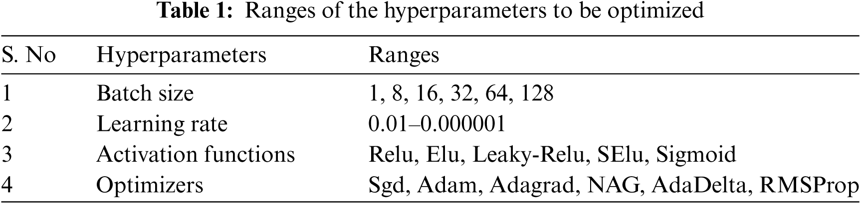
The selected parameters for this step of optimization includes: Ai = 0.3, freqmin = 0, freqmax = 1, β = 0.5, and μ = 0.5. In our approach, the initialization of the pulse rate for each bat is in increasing order to the fitness of each bat. This is done to reduce the probability of solutions with better fitness to perform random local searches around other top best solutions. This strategy may help reduce the probability of early convergence which is the main limitation of the bat algorithm. We found through experiments that nudges of parameters in the vicinity of better fit CNN models give improved results. Therefore, the pulse rate initialization in increasing order with respect to fitness will lower the prospect of overlooking the problem space in the vicinity of better fit models. The process of optimization starts by initializing a population of 10 bats thereafter, the position of each bat is adjusted based on the velocity and frequency, which are updated at each iteration using the standard bat algorithm. The position of each bat represents the hyperparameter setting for a CNN model, i.e., a real-valued vector representing the batch size, activation function, learning rate, and optimizer. The activation function and optimizer are then mapped to real numbers, after which all the dimensions of each bat are encoded in the same range. Tab. 1 presents the search space for each dimension of the bats.
At the initialization step, the position of each bat is assigned randomly, and the velocity of each bat is initialized as 0. We then initialize the pulse rate and loudness after evaluating the fitness of the position of each bat. The performance of each set of hyperparameters proposed by the bat algorithm was then validated by the MSE of a fixed CNN architecture. For this purpose, we have selected top-performing architecture from an existing work [30] (we name it ‘M1’), to optimize four hyperparameters of CNN, namely, the batch size, learning rate, activation function, and the optimizer. After 20 iterations on a population of 10 bats, the top 4 high-performing hyperparameter settings obtained at the last iteration are depicted in Tab. 2.
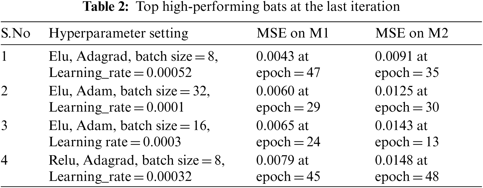
With each hyperparameter setting, the model is trained for 50 epochs. To verify these hyperparameter settings, another top-performing model (denoted as M2) of the existing work [30] is trained, and its performance is evaluated. M1 and M2 are depicted in Figs. 2a and 2b.

Figure 2: Models for the validation of step 1 of our methodology (a) model 1 (M1) (b) model 2(M2)
For the next experiments of the CNN architecture optimization, we selected the second-best hyperparameter setting instead of the best setting, as it requires a relatively low number of epochs to provide satisfactory results.
6.2 Optimizing the CNN Architecture Using the Bat Algorithm
In this subsection, the optimization of five architectural properties using the bat algorithm is explained, including the number of Conv layers, number of filters in each Conv layer, filter sizes in each layer, number of FC layers, and number of neurons in each FC layer; the ranges of these parameters in our approach are (3–13), (16–128), (3 × 3–7 × 7), (1–5), and (10–120), respectively. Algorithm 1 is adopted to optimize the CNN architecture, with pop_size = 10, numofgen = 20, freqmin = 1, freqmax = 4, initial loudness = 4, dimension (D) = 5, β = 0.9, μ = 0.9, and pulse rate is initialized in an ascending order with respect to the fitness of the bats. Position xi of each bat represents a particular CNN architecture, and each dimension of the bat corresponds to the CNN architectural property. At the initialization step, position xi of each bat is then initialized randomly in the range specified for the respective dimension. Subsequently, each dimension is rescaled in the range of 10–250 for further processing in the next iterations. The velocity of each bat is initialized as 0, after which it is adjusted using Eq. (2) as mentioned in Section 4 of this paper. The velocity is bound to the range of −18 to 18.
When we automate the architecture formation of the CNN, we can encounter dimensionality problems. Thus, if the output feature map is not padded, then depending on the size of the Conv filters, the dimension is reduced. Alternatively, if the layers are padded so that the input and dimensionality of the output feature map are preserved, the CNN architecture will not fit in the memory for training as the layers increase. Therefore, before connecting the FC layers, it is important to reduce the dimensionality. We have solved these dimensionality problems using the strategy depicted in Algorithm 2.

6.3 Optimizing the CNN Architecture Using the PSO Algorithm
In this subsection, the optimization of five architectural properties using the PSO algorithm is explained, including the number of Conv layers, number of filters in each Conv layer, filter sizes in each layer, number of FC layers, and the number of neurons in each FC layer. Position xi of each particle represents a particular CNN architecture, and each dimension of the particle corresponds to the CNN architectural property. At the initialization step, position xi of each particle is initialized the same as the first population of the bat algorithm in the previous step. This is carried out to ensure the same average fitness of individuals at the first iteration of the PSO and bat algorithms. After the initialization of the particle positions, each dimension is then rescaled in a range of 10–250 for further processing in the next iterations. The velocity of each particle is initialized as 0, which is then adjusted using Eq. (7). The velocity is bound to the range of −18 to 18. Most researchers obtained optimal results with a value of ‘2’ for c1 and c2 [43,44]. Therefore, in our methodology, this value is selected for the PSO algorithm. The encoding scheme for each position of particles is the same as that used in the bat algorithm. Each model is trained for 50 epochs using the top-second hyperparameter setting obtained in step 1 of our methodology implemented in Section 6.1. Algorithm 3 presents the methodology of the application of the PSO algorithm for the hyperparameter optimization of CNN.

For the steering angle predictive neural network to be implemented practically, it needs to be robust. One way of achieving robustness is to train the CNN model with the extensive dataset containing various scenarios. To achieve this, the CNN model with the least MSE obtained after the optimization was retrained with more data (i.e., 25000 more data samples). The top hyperparameter setting obtained in Section 6.1 was used for training the CNN model. Afterward, infield testing was performed using the trained model to drive the vehicle on a road. The camera was mounted on the front, aligned at the exact center of the vehicle.
The Python library, named “OpenCV,” was used in capturing live frames (of dimension 640 × 480), which were continuously being utilized by the trained CNN model for the prediction of the steering angle. The dimensions of training, as well as testing frames, should be similar. Therefore, one-third of each frame from the live feed is cropped from the top and then rescaled to 300 × 300. Fig. 3 shows some examples of the original and equivalently cropped/rescaled testing and training frames.

Figure 3: Cropping and rescaling of the frames (a) testing frame (b) training frame
The average prediction time taken by our model on live camera frames was 0.1 s. The model gave continuous values within the range of −2 to 2, with 2 as a command to steer toward the extreme left and −2 as a command to steer toward the extreme right. Values close to 0, e.g., 0.0052, −0.00093, and 0.0102, are identified as commands to drive straight. The predicted steering angle is sent to Arduino ESP 32 DEVKIT V1 which controls the rotation of wheels through the help of a rotational potentiometer. The experiments were conducted for a total of 1 h of driving at different times of the day and different positions of the vehicle on the road. As per our findings, we found that the best prediction results of the model were obtained when the position of the vehicle was in the middle of the road. However, it did not perform well near the boundaries of the road, particularly at the right margins of the road. Such wrong predictions might be because, during the collection of the dataset, the vehicle was mostly driven at the center of the road. As the width of the road, lane marking color, and other properties of the testing track is different from the training track, the ability of the CNN model to generalize for new scenarios is convincible. In Fig. 4, some of the scenarios with correct as well as wrong prediction results are shown.

Figure 4: Samples of our prediction results (a) correct predictions (b) wrong Predictions
This section provides details of our methodology and findings. We optimized the CNN via a two-step process. In the first step, we tuned four hyperparameters, and, in the second step, we optimized five architectural properties of the CNN. We began our experiment by tuning four hyperparameters for which a fixed CNN model was employed. Thereafter, the effectiveness of the tuned hyperparameter settings for other CNN architectures was verified by training another model (M2).
In the solution vector of the best bat in step 1 of our approach, we obtained a 0.00052 learning rate for the Adagrad optimizer. This is then used as the initial learning rate by the optimizer and is updated for every parameter based on the past gradients. We observed that the Adagrad optimizer consumed more training time and required a higher number of epochs as compared to those of Adam, which can be observed in Tab. 4. Therefore, for the experiments of the CNN architecture optimization, we selected the second-best hyperparameter setting instead of the top-most setting because it provides a satisfactory estimate of the performance of a model with fewer epochs. For the comparison of the PSO and Bat algorithms for the CNN architecture optimization, the average fitness of the individuals in a population is plotted at each iteration (see Fig. 5).
It is useful to observe the cumulative effect of several layers of the CNN model on the performance of the model. Hence, we have plotted the MSE of models obtained through both optimization algorithms concerning the total count of layers (see Fig. 6).

Figure 5: Average fitness of the individuals in a population at each iteration

Figure 6: Box plot of the mean square error for each layer
In the above figure, the number of layers refers to the sum of Conv and FC layers only. We have observed that the deep models perform better than the shallow ones.
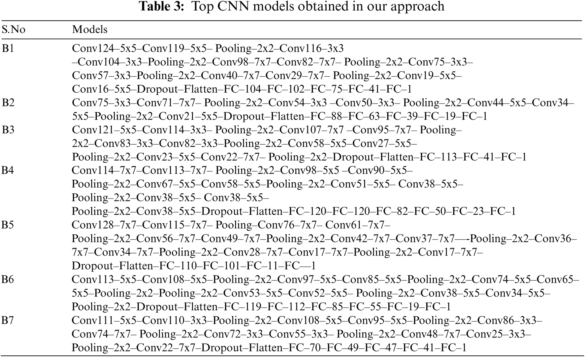
After the process of training, each CNN model in our approach takes 300 x 300 RGB images as input and produces a real number as output in the range of −2 to 2. This number is the steering angle predicted by CNN with respect to a given image. Top CNN models obtained in our approach with the least MSEs have been depicted in Tab. 3.
In the above table, a number of Conv filters used in each Conv layer are mentioned followed by the size of the filter. Filter size of each max-pooling layer is also mentioned followed by the word “Pooling”. Each architecture has a flattened layer between the Conv and FC layers. The number of neurons in each FC layer is mentioned right next to it. Moreover, each model ends with the FC layer having one neuron serving the purpose of the output layer. A dropout layer is added before the flatten layer in each model. We used the “ELU” activation function for each layer except for the last FC layer where a linear activation function was used. We have named models for further reference in Tab. 3 as B1, B2, up to B7.
As the pooling layer with filter size 2 × 2 reduces the size of each feature map by a factor of 2, i.e., each dimension is halved, we cannot apply a pooling layer after each Conv layer. As the input image size used in our approach is 300 × 300, after seven applications of the pooling layer, each feature map dimension will then reduce to 2 × 2, whereas the maximum number of Conv layers used in our approach is 13. Therefore, we adopted the strategy of applying the pooling layer depicted in Algorithm 3. According to this, if the number of Conv layers proposed by the either of Bat or PSO algorithm in the current solution vector is less than or equal to 5, then max pooling is applied after each Conv layer, else it is applied after two Conv layers. Another precautionary measure taken in our approach to abolishing dimensionality problems is zero paddings of the Conv layers. The output of the Conv layer is determined by the formula:
where W is the input volume, Fsize is the filter size, P is the padding, and S is the stride. In our case, the stride of 1 is applied throughout the experiments. We applied varied paddings on layers depending on the filter size. That is, padding of 2 × 2 is applied if the filter size is 3 × 3, 3 × 3 if the filter size is 5 × 5, and 5 × 5 if the filter size is 7 × 7. Therefore, the output size of the Conv layer in our approach remains the same as the input layer size.
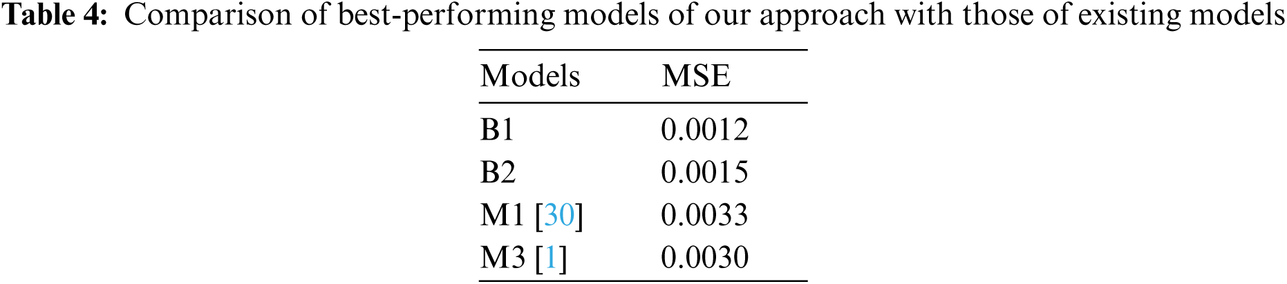
Although we can see in Fig. 5 that the models are still improving at the last epochs using the Adagrad optimizer without overfitting, we trained all the models for 50 epochs during the optimization because of time constraints. However, improved performance could be obtained using more epochs on the Adagrad optimizer. Therefore, to revalidate our results, we trained the best-performing model architecture with the Adagrad optimizer for 200 epochs. The results are then compared with existing hand-tuned steering angle predictive CNN models (M1 and M3) from previous studies [1,30]. Model M1 has already been defined in Section 6.1; M3 is a 9-layered CNN model containing 5 Conv and 4 FC layers. Tab. 4 shows the comparative results of the top two best-performing models obtained in our experiments (B1 and B2), with the best-performing models of the previous study (M1 and M3).
Through careful observation of our findings, we can conclude that CNN models having a high number of layers perform better than the models with a low number of layers. This may not necessarily be true for Conv layers more than 13 and FC layers more than 5, because this is the maximum range we selected for our methodology. The evaluation criterion, i.e., MSE of the best CNN architecture obtained at the end of all iterations, articulates the effectiveness of our approach in optimizing the CNN architecture and other hyperparameters using the metaheuristic algorithms. We found, during our experimentation, that even though the deep models require more training time and epochs, they provide better results as compared to the shallow ones.
Deep learning models as opposed to traditional algorithms articulated with preformulated rules are efficient in representing the relationship between the response and its predictor. However, the problem space having all the possible combinations of real values for each parameter of these models is diverse; thus, it is infeasible to explore with exhaustive search as the number of layers increase. Therefore, we applied the metaheuristic algorithms to tune the CNN architectural parameters and other hyperparameters. Through careful observation of our findings, we can conclude that CNN models having a high number of layers perform better than the models with a low number of layers. This may not necessarily be true for Conv layers more than 13 and FC layers more than 5, because this is the maximum range we selected for our methodology. The evaluation criterion, i.e., MSE of the best CNN architecture obtained at the end of all iterations, articulates the effectiveness of our approach in optimizing the CNN architecture and other hyperparameters using the metaheuristic algorithms. We found, during our experimentation, that even though the deep models require more training time and epochs, they provide better results as compared to the shallow ones. In future, we would collect our own dataset and compare the performance of the CNN model trained on Udacity dataset with the same model trained on our own dataset. This would be done through the infield testing on same vehicle in different scenarios.
Funding Statement: The authors would like to acknowledge the support of the Deputy for Research and Innovation, Ministry of Education, Kingdom of Saudi Arabia for this research through a grant (NU/IFC/INT/01/008) under the institutional Funding Committee at Najran University, Kingdom of Saudi Arabia.
Conflicts of Interest: The authors declare that they have no conflicts of interest to report regarding the present study.
1. A. Intisar, M. K. B. Islam and J. Rahman, “A deep convolutional neural network based small scale test-bed for autonomous car,” in Proc. of the Int. Conf. on Computing Advancements, Dhaka, Bangladesh, pp. 1–5, 2020. [Google Scholar]
2. R. Chaudhari, S. Dubey, J. Kathale and R. Rao, “Autonomous driving car using convolutional neural networks,” in Second Int. Conf. on Inventive Communication and Computational Technologies (ICICCTIEEE, Conf. Proc., Tamil Nadu, India, pp. 936–940, 2018. [Google Scholar]
3. D. Wang, J. Wen, Y. Wang, X. Huang and F. Pei, “End-to-end self-driving using deep neural networks with multi-auxiliary tasks,” Automotive Innovation, vol. 2, no. 2, pp. 127–136, 2019. [Google Scholar]
4. V. Singhal, S. Gugale, R. Agarwal, P. Dhake and U. Kalshetti, “Steering angle prediction in autonomous vehicles using deep learning,” in 5th Int. Conf. on Computing, Communication, Control and Automation (ICCUBEAIEEE, Conf. Proc., Pune, India, pp. 1–6, 2019. [Google Scholar]
5. U. M. Gidado, H. Chiroma, N. Aljojo, S. Abubakar, S. I. Popoola et al., “A survey on deep learning for steering angle prediction in autonomous vehicles,” IEEE Access, vol. 8, pp. 163797–163817, 2020. [Google Scholar]
6. A. Bakhshi, N. Noman, Z. Chen, M. Zamani and S. Chalup, “Fast automatic optimisation of cnn architectures for image classification using genetic algorithm,” in IEEE Congress on Evolutionary Computation (CEC) Conf. Proc., Wellington, New Zealand, pp. 1283–1290, 2019. [Google Scholar]
7. H. Saleem, F. Riaz, L. Mostarda, M. A. Niazi, A. Rafiq et al.., “Steering angle prediction techniques for autonomous ground vehicles: A review,” IEEE Access, vol. 9, pp. 78567–78585, 2021. [Google Scholar]
8. F. Johnson, A. Valderrama, C. Valle, B. Crawford, R. Soto et al.., “Automating configuration of convolutional neural network hyperparameters using genetic algorithm,” IEEE Access, vol. 8, pp. 156139–156152, 2020. [Google Scholar]
9. J. Wu, J. Long and M. Liu, “Evolving RBF neural networks for rainfall prediction using hybrid particle swarm optimization and genetic algorithm,” Neurocomputing, vol. 148, no. 19, pp. 136–142, 2015. [Google Scholar]
10. Z. Arabasadi, R. Alizadehsani, M. Roshanzamir, H. Moosaei and A. A. Yarifard, “Computer aided decision making for heart disease detection using hybrid neural network-genetic algorithm,” Computer Methods and Programs in Biomedicine, vol. 141, pp. 19–26, 2017. [Google Scholar]
11. S. Wang, Y. Zhang, Z. Dong, S. Du, G. Ji et al.., “Feed-forward neural network optimized by hybridization of PSO and ABC for abnormal brain detection,” International Journal of Imaging Systems and Technology, vol. 25, no. 2, pp. 153–164, 2015. [Google Scholar]
12. A. Bhandare and D. Kaur, “Designing convolutional neural network architecture using genetic algorithms,” in Proc. on the Int. Conf. on Artificial Intelligence (ICAIthe Steering Committee of the World Congress in Computer Science, Computer Engineering and Applied Computing (WorldCompNewyork, United States, pp. 150–156,. 2018. [Google Scholar]
13. T. Y. Kim and S. B. Cho, “Particle swarm optimization-based CNN-LSTM networks for forecasting energy consumption,” IEEE Congress on Evolutionary Computation (CECWellington, New Zealand, pp. 1510–1516, 2019. [Google Scholar]
14. Y. Wang, H. Zhang and G. Zhang, “CPSO-CNN: An efficient PSO-based algorithm for fine-tuning hyper-parameters of convolutional neural networks,” Swarm and Evolutionary Computation, vol. 49, pp. 114–123, 2019. [Google Scholar]
15. F. C. Soon, H. Y. Khaw, J. H. Chuah and J. Kanesan, “Hyper-parameters optimisation of deep CNN architecture for vehicle logo recognition,” IET Intelligent Transport Systems, vol. 12, no. 8, pp. 939–946, 2018. [Google Scholar]
16. T. Yamasaki, T. Honma and K. Aizawa, “Efficient optimization of convolutional neural networks using particle swarm optimization,” in IEEE Third Int. Conf. on Multimedia Big Data (BigMMLaguna Hills, CA, USA, pp. 70–73, 2017. [Google Scholar]
17. T. Sinha, A. Haidar and B. Verma, “Particle swarm optimization-based approach for finding optimal values of convolutional neural network parameters,” in IEEE Congress on Evolutionary Computation (CECWellington, New Zealand, pp. 1–6, 2018. [Google Scholar]
18. P. R. Lorenzo, J. Nalepa, M. Kawulok, L. S. Ramos and J. R. Pastor, “Particle swarm optimization for hyper-parameter selection in deep neural networks,” in Proc. of the Genetic and Evolutionary Computation Conf., Conf. Proc., Berlin, Germany, pp. 481–488, 2017. [Google Scholar]
19. G. Wang and L. Guo, “A novel hybrid bat algorithm with harmony search for global numerical optimization,” Journal of Applied Mathematics, vol. 2013, article ID 696491, pp. 1–21, 2013. [Google Scholar]
20. R. Sedaghati and F. Namdari, “An intelligent approach based on metaheuristic algorithm for non-convex economic dispatch,” Journal of Operation and Automation in Power Engineering, vol. 3, no. 1, pp. 47–55, 2015. [Google Scholar]
21. N. S. Jaddi, S. Abdullah and A. R. Hamdan, “Multi-population cooperative bat algorithm-based optimization of artificial neural network model,” Information Sciences, vol. 294, pp. 628–644, 2015. [Google Scholar]
22. C. Zhao, J. Gong, C. Lu, G. Xiong and W. Mei, “Speed and steering angle prediction for intelligent vehicles based on deep belief network,” in IEEE 20th Int. Conf. on Intelligent Transportation Systems (ITSCYokohama, Japan, pp. 301–306, 2017. [Google Scholar]
23. M. V. Smolyakov, A. I. Frolov, V. N. Volkov and I. V. Stelmashchuk, “Self-driving car steering angle prediction based on deep neural network an example of carND udacity simulator,” in IEEE 12th Int. Conf. on Application of Information and Communication Technologies (AICTAlmaty, Kazakhstan, pp. 1–5, 2018. [Google Scholar]
24. V. Rausch, A. Hansen, E. Solowjow, C. Liu, E. Kreuzer et al.., “Learning a deep neural net policy for end-to-end control of autonomous vehicles,” in American Control Conf. (ACCSeattle, USA, pp. 4914–4919, 2017. [Google Scholar]
25. A. K. Jain, “Working model of self-driving car using convolutional neural network, raspberry pi and arduino,” in Second Int. Conf. on Electronics, Communication and Aerospace Technology (ICECACoimbatore, India, pp. 1630–1635, 2018. [Google Scholar]
26. R. Chaudhari, S. Dubey, J. Kathale and R. Rao, “Autonomous driving car using convolutional neural networks,” in Second Int. Conf. on Inventive Communication and Computational Technologies (ICICCTIEEE, Coimbatore, India, pp. 936–940, 2018. [Google Scholar]
27. Z. Yang, Y. Zhang, J. Yu, J. Cai and J. Luo, “End-to-end multi-modal multi-task vehicle control for self-driving cars with visual perceptions.” in 24th Int. Conf. on Pattern Recognition (ICPRMilan, Italy, pp. 2289–2294, 2018. [Google Scholar]
28. M. T. Duong, T. D. Do and M. H. Le, “Navigating self-driving vehicles using convolutional neural network.” in 4th Int. Conf. on Green Technology and Sustainable Development (GTSDHo Chi Minh City, Vietnam, pp. 607–610, 2018. [Google Scholar]
29. A. Agnihotri, P. Saraf and K. R. Bapnad, “A convolutional neural network approach towards self-driving cars.” in IEEE 16th India Council Int. Conf. (INDICONGujrat, India, pp. 1–4, 2019. [Google Scholar]
30. P. M. Kebria, A. Khosravi, S. M. Salaken and S. Nahavandi, “Deep imitation learning for autonomous vehicles based on convolutional neural networks,” IEEE/CAA Journal of Automatica Sinica, vol. 7, no. 1, pp. 82–95, 2019. [Google Scholar]
31. V. Bibaeva, “Using metaheuristics for hyper-parameter optimization of convolutional neural networks,” in IEEE 28th Int. Workshop on Machine Learning for Signal Processing (MLSPAalborg, Denmark, pp. 1–6,. 2018. [Google Scholar]
32. N. S. Jaddi, S. Abdullah and A. R. Hamdan, “Optimization of neural network model using modified bat-inspired algorithm,” Applied Soft Computing, vol. 37, pp. 71–86, 2015. [Google Scholar]
33. S. Albawi, T. A. Mohammed and S. Al-Zawi, “Understanding of a convolutional neural network,” in Int. Conf. on Engineering and Technology (ICETAntalya, Turkey, pp. 1–6, 2017. [Google Scholar]
34. M. Sun, Z. Song, X. Jiang, J. Pan and Y. Pang, “Learning pooling for convolutional neural network,” Neurocomputing, vol. 224, pp. 96–104, 2017. [Google Scholar]
35. V. Rausch, A. Hansen, E. Solowjow, C. Liu and E. Kreuzer, “Learning a deep neural net policy for end-to-end control of autonomous vehicles,” in American Control Conf. (ACC). IEEE, Conf. Proc., Seattle, USA, pp. 4914–4919, 2017. [Google Scholar]
36. A. Khanum, C. Y. Lee and C. S. Yang, “End-to-end deep learning model for steering angle control of autonomous vehicles,” in 2020 Int. Symp. on Computer, Consumer and Control (IS3CTaichung City, Taiwan, pp. 189–192, 2020. [Google Scholar]
37. V. John, A. Boyali, H. Tehrani, K. Ishimaru, M. Konishi et al.., “Estimation of steering angle and collision avoidance for automated driving using deep mixture of experts,” IEEE Transactions on Intelligent Vehicles, vol. 3, no. 4, pp. 571–584, 2018. [Google Scholar]
38. S. Chen, S. Zhang, J. Shang, B. Chen and N. Zheng, “Brain-inspired cognitive model with attention for self-driving cars,” IEEE Transactions on Cognitive and Developmental Systems, vol. 11, no. 1, pp. 13–25, 2017. [Google Scholar]
39. T. V. Orden and A. Visser, “End-to-end imitation learning for autonomous vehicle steering on a single camera stream,” in Proc. of 16th Int. Conf. on Intelligent Autonomous System (IASSingapore, pp. 224–235,. 2021. [Google Scholar]
40. X. S. Yang, “A new metaheuristic bat-inspired algorithm,” In Nature Inspired Cooperative Strategies for Optimization (NICSO 2010), Berlin, Heidelberg: Springer, pp. 65–74, 2010. [Google Scholar]
41. S. Sengupta, S. Basak and R. A. Peters, “Particle swarm optimization: A survey of historical and recent developments with hybridization perspectives,” Machine Learning and Knowledge Extraction, vol. 1, no. 1, pp. 157–191, 2019. [Google Scholar]
42. Udacity self-driving car dataset (ch2_002.bag.tar.gzAccessed: 5-Oct-2020. [Online]. Available: https://github.com/udacity/self-driving-car/blob/master/datasets/CH2. [Google Scholar]
43. F. Chen, X. Sun, D. Wei and Y. Tang, “Tradeoff strategy between exploration and exploitation for PSO,” in Seventh Int. Conf. on Natural Computation, Shanghai, China, vol. 3, pp. 1216–1222, 2011. [Google Scholar]
44. L. Xiong, R. S. Chen, X. Zhou and C. Jing, “Multi-feature fusion and selection method for an improved particle swarm optimization,” Journal of Ambient Intelligence and Humanized Computing, vol. 2019, no. 1, pp. 1–10, 2019. [Google Scholar]
 | This work is licensed under a Creative Commons Attribution 4.0 International License, which permits unrestricted use, distribution, and reproduction in any medium, provided the original work is properly cited. |