Computers, Materials & Continua DOI:10.32604/cmc.2022.023059
Article

CDLSTM: A Novel Model for Climate Change Forecasting

Mohd Anul Haq*

Department of Computer Science, College of Computer and Information Sciences, Majmaah University, AL Majmaah, 11952, Saudi Arabia
*Corresponding Author: Mohd Anul Haq. Email: m.anul@mu.edu.sa
Received: 26 August 2021; Accepted: 27 September 2021

Abstract: Water received in rainfall is a crucial natural resource for agriculture, the hydrological cycle, and municipal purposes. The changing rainfall pattern is an essential aspect of assessing the impact of climate change on water resources planning and management. Climate change affected the entire world, specifically India’s fragile Himalayan mountain region, which has high significance due to being a climatic indicator. The water coming from Himalayan rivers is essential for 1.4 billion people living downstream. Earlier studies either modeled temperature or rainfall for the Himalayan area; however, the combined influence of both in a long-term analysis was not performed utilizing Deep Learning (DL). The present investigation attempted to analyze the time series and correlation of temperature (1796–2013) and rainfall changes (1901–2015) over the Himalayan states in India. The Climate Deep Long Short-Term Memory (CDLSTM) model was developed and optimized to forecast all Himalayan states’ temperature and rainfall values. Facebook’s Prophet (FB-Prophet) model was implemented to forecast and assess the performance of the developed CDLSTM model. The performance of both models was assessed based on various performance metrics and shown significantly higher accuracies and low error rates.

Keywords: Himalayas; climate change; cdlstm; facebook; temperature; rainfall

1  Introduction

Climate change affected India, specifically the fragile Himalayan mountainous region, which has high significance due to climatic indicators, the origin of rivers, municipal, agricultural, hydroelectric purposes, minerals, and tourism [1–3]. The Himalayan area is the world’s highest mountain system that stretches over 2,500 km, covering twelve states of India either partially or fully. These are Jammu and Kashmir (J&K, now Jammu, Kashmir, and Ladakh), Himachal Pradesh (Him), Uttarakhand (UK), Nagaland, Manipur, Mizoram, Tripura (NMMT), Assam, and Meghalaya (A&M), Arunachal Pradesh (Arun) and sub–Himalayan West Bengal and Sikkim (WB&S). The high-altitude area of the Himalayas is covered with snow and glaciers. The water from snow and glaciers is essential for municipal, agricultural, and hydroelectric [1–3]. The Himalayan area impacts the climate of the entire Indian subcontinent by controlling the monsoon and rainfall patterns. The Himalayan ecosystem is very fragile and sensitive to climate change parameters such as temperature and rainfall. The criticality of rainfall analysis is evident from the June 2013 Uttarakhand disaster. The UK state received 847% extra rainfall in the third week of June, resulting in the Kedarnath flood disaster that took more than 5000 lives.

In current times, the utility of machine learning (ML) approaches has a significant presence in almost every area, and the successful utilization of deep learning (DL) has opened new dimensions for efficient time series forecasting. ML/DL has been used extensively for climate analysis and forecasting [4–9]. A study by [10] provides a comprehensive report on climate change in the Himalayas and suggests modeling future climate status, especially for the Himalayan region. [11,12] applied Dl techniques such as DNN and RNN for weather forecasting; however, the scope and data used in their investigation were limited. However, significant issues with these studies are rigorous parameter tuning, cross-validation of the model on different data, and computational efficiency. Additionally, while previous studies have addressed annual climate issues for the entire expanse of India, very few studies have explicitly focused on all the Himalayan states due to the complexity of data for the Himalayan region [13–15]. Understanding the climate variability for Himalayan states on a monthly temporal scale is crucial for hydrological and climatic models [16]. The present study focuses on all the Himalayan states to provide comprehension of changing temperature and rainfall patterns. The present investigation contributes to three significant aspects: detecting rainfall and temperature trends, analyzing the correlation between temperature and rainfall, and forecasting the temperature and rainfall using a novel CDLSTM model and Facebook Prophet (FB-Prophet) Model.

1.1 LSTM

LSTM networks are a type of Recurrent Neural Network (RNN) that uses special units (cells) and standard units to overcome the limitation of traditional RNN [17–20]. There are three gates, which are contained by a cell in LSTM. The first gate is the input gate, the second is termed the forget gate, whereas the third is the output gate. The LSTM network composition function’s description is based on the input node, and the three gates are contained by a cell, cell state, and output layer. Eqs. (1)–(7) are as follows [20,21].

Input node

g(t)=tanh⁡(Wgxx(t)+Wghh(t−1)+bg(1)

Input gate

i(t)=σ(Wixx(t)+Wihh(t−1)+bi(2)

Forget gate

f(t)=σ(Wfxx(t)+Wfhh(t−1)+bf(3)

Output gate

o(t)=σ(Woxx(t)+Wohh(t−1)+bo(4)

Cell state

s(t)=g(t)⊙i(t)+s(t−1)⊙o(t)(5)

Hidden gate

h(t)=tanh⁡(s(t))⊙o(t)(6)

Output layer

y(t)=σ(Whyh(t)+by)(7)

1.2 Facebook’s Prophet Model

Facebook’s Prophet is an open-source forecasting tool based on a decomposable additive model, similar to a generalized additive model (GAM). Prophet can fit nonlinear time series with seasonality. The Prophet forecast model can be expressed as Eq. (8).

F(t)=L(t)+S(t)+E(t)+X(t)(8)

where, F(t) = forecast, L(t) = long term trend, S(t)= short term trend, E(t) = error, and X(t) = any other influencing variable to forecast.

Prophet has two models: logistic growth model (LGM) and piece-wise linear (PWL) model. The selection of the model depends on the time series data. The LGM model can be used if the time series shows non-linearity, saturation, and no change after reaching the saturation point. If the time series exhibits linear tendency and a previous track of shrink and growth, then PWL is a better option. The LGM can be expressed as Eq. (9).

L(t)=CC1+e−g(t−o)(9)

where CC = carry capacity, g = growth rate, and o is an offset parameter. The PWL can be expressed as Eq. (10).

y={β0+β1xx≤cβ0−β2c(β1+β2)x>c}(10)

2  Dataset

2.1 Rainfall

The monthly rainfall dataset was obtained from more than 3000 rain-gauge stations spread over India, covering 115 years (Jan 1901–Dec 2015). The dataset was released by Indian Meteorological Department (IMD) (https://www.imdpune.gov.in/).

2.2 Temperature

The Berkeley Earth monthly average data from Jan 1796–Aug 2013 was procured from https://guides.lib.berkeley.edu/publichealth/healthstatistics/rawdata. It was generated based on a variety of data, including bias-corrected station data, regional data. The data was developed from various sources with quality control, and monthly averages were created from daily data. A standard temporal observation period of Jan 1901–Aug 2013 was considered to understand the relationship between temperature and rainfall.

3  Methodology

3.1 Data Preprocessing

For in-depth analysis of seasonal patterns of temperature and rainfall, the data was divided into four seasons based on India’s meteorological and international standards, i.e., Dec-Feb as winter, March to May as spring, June-Sep as monsoon, and Oct-Nov as post-monsoon or autumn. Temperature and rainfall data were used; therefore, the term monsoon was used instead of summer for rainfall analysis purposes. Data transformation is crucial before implementing any ML model. Three data transformations were applied in the current investigation. The first transformation was removing missing values and replacing them with average values from the respective records. The second step was transforming time-series data into input and output so that the output of a step could become the input for the next step to forecast the value of the current time step. As described earlier, the total common data in the time series covered 1352 monthly values. The first 980 months’ dataset for all Himalayan states was taken for the training, while testing took 240 months, and validation used the dataset of 120 months of the LSTM model; the remaining twelve months of data were kept separate from the training process for the unbiased external validation of the LSTM prediction. The third transformation was the scaling of time series data from –1 to 1. These three transformations were inverted after the prediction step to get the values at the original scale so that the uncertainty calculation could be adequately assessed.

3.2 Trend Analysis

Mann-Kendall tests [22,23] were carried out for trend analysis, detecting trends and changes in temperature and rainfall over the years of analysis. Sen’s slope values [24] were used to understand the trend of GWSC change for all Himalayan states from Jan 1901 to Dec 2015. Statistics of Mann-Kendall S value [22,23] were evaluated for chronologically placed observations in the time series Eq. (11). The observations VAR(S) variance in the time series was also estimated as per Eq. (13). Standardized test Z Eq. (14) [25] for the statistical analysis was also performed.

S=∑i=1n−1∑j=i+1nSgn(Xj−Xi)(11)

Sgn(Xj−Xi)={+1,>(Xj−Xi)0,=(Xj−Xi)−1,<(Xj−Xi),(12)

VAR(S)=118[n(n−1)(2n+5)−∑p=1qtp(tp−1)(2tp+5)](13)

Z{S−1VAR(S)ifS>00ifS=0S+1VAR(S)ifS<0.(14)

Here, Xi and Xj are chronologically placed values of variables in the time series, n represents the total count of observations, ties for pth value is shown as tp, and tied values number is shown as q. When Z is positive, it means an increasing trend in the climatic variable and vice versa.

3.3 Correlation Analysis Between Variables

An attempt was made to study the correlation analysis based on Moment Correlation Coefficient (MCC) among temperature and rainfall values for all the twelve Himalayan states from Jan 1901 to Aug 2013, as per the availability of a common temporal dataset.

The MCC summarizes the direction and degree of linear relations between actual and modeled datasets. The correlation coefficient can take values between –1 (perfectly negative correlation) through 0 (no correlation) to +1 (perfectly positive correlation). The MCC formula to compute the correlation coefficient is given in Eq. (15).

R=N∑XY−∑X∑Y[N∑X2−(∑X)2](N∑Y2−(∑Y2)(15)

Here, N represents the number of pairs of data. The terms X and Y are parameters.

3.4 Development and Tuning of CDLSTM Model

Keras library with TensorFlow and Python version was used to develop the LSTM models in the current study. The libraries used in the current investigation were Plotly, NumPy, Seaborn, Pandas, Matplotlib, and scikit-learn. A four-step procedure was applied to develop the LSTM model.

The first step was to define the LSTM network to aid LSTM model development. Eight LSTM layers were used in the current investigation, in which four layers were dense, and three were the dropout layers, see Fig. 1. The dropout layer “drops out” inputs to a layer, which may be input variables from a previous layer. A value of 0.5 was chosen with two dropout layers. The second step was the network compilation. It required several parameters, such as an optimization algorithm to train the network and the loss function to evaluate the network. Several optimizers were tested based on their performances. The third step was the fitting of the LSTM model. The fourth and essential step was the prediction using the LSTM model. We forecasted the output step by step for the test data. The model fed the current forecasted value back into the input window by moving it one step forward to forecast the next step using the moving-forward window technique [26]. Here we used a moving forward window of size 12. We forecasted the average temperature individually for all Himalayan states from Sep 2012 to Aug 2013 using one step ahead regression based on window size.

Figure 1: The architecture of the CDLSTM model used in the current investigation

Several hyper-parameters such as optimizer, number of units, learning rate, momentum, and activation functions must be chosen a priori and then tuned based on the RMSE values. Tuning the hyper-parameters of any neural network model is essential for evaluating the performance and stability of the DL model. The first configuration tuned was the number of nodes, which affected the LSTM model’s learning capability. A higher number of nodes ensures excellent learning ability for complex data at the cost of computation time and can cause overfitting. Different nodes (2, 4, 6, 8, and 10) were tested for different configurations. A lesser average RMSE value of 1.4 and the lowest variance based on 20 experimental runs were obtained with four nodes. However, since it could indicate overfitting, dropout was applied to prevent overfitting, where the neurons were randomly chosen and ignored during model training to address the issue of overfitting. The number of epochs (10, 20, 30, 40, and 50), optimization algorithm (Adam, RMSProp, Adagrad, SGD), and individual learning rate (1e-2 to 1e-6) were also rigorously tuned. It was observed that the tuned LSTM model with eight nodes, trained for 20 epochs with an ADAM optimizer having LR of 1e-2, showed the best performance based on RMSE and computational efficiency in the current investigation.

3.5 Facebook’s Prophet Model

The Prophet forecast model looks straightforward; however, the computation can be complex due to the selection of parameters. The selection of the LGM or PWL model depends on the time series data. The LGM model was applied for rainfall data due to the time series; however, PWL model was applied for temperature forecasting as it exhibits linear tendency.

The uncertainty in the forecasting values can be obtained by forwarding the GAM model, which can be expressed as Eq. (16).

∀j>T,[∂j=0whereT−S.T∂j∼Laplace(0,φ)whereS.T](16)

where ∂ is a rate scale parameter.

The FB-Prophet model was imported. The Prophet model was fitted with training data, and forecasting was implemented based on 12 periods and month start (MS) as frequency.

3.6 Uncertainty Assessment of the LSTM Model

The MCC, Root Mean Square Error (RMSE), Mean Absolute Percentage Error (MAPE), and Nash-Sutcliffe coefficient (NSE) were utilized to evaluate the uncertainty of the LSTM model output. The Mean Absolute Deviation (MAD) was also considered to analyze the LSTM model’s accuracy between measured and predicted values.

RMSE is a method to calculate the error or accuracy in predicting models based on standard deviation Eq. (17). The final output is given in the form of the standard deviation of the error’s magnitude, as per Eq. (17); the individual calculations are outputted as residuals based on [27].

RMSE=∑n=1n(Yi−Oi)2n(17)

Here, P_i is the ith LSTM predicted value, and Oi is the ith original value.

The MAPE method was used to calculate the prediction accuracy of the LSTM forecast. The calculation was based on the difference between the original values and values forecasted by the LSTM and dividing the original value difference. It was then multiplied by the number of observations and 100 to obtain the percentage error (18) [28].

MAPE=100n∑n=1n|At−FtAt|(18)

Here, At represents actual value. Similarly, symbol Ft represents the forecasted value or the predicted value. MAD was used to calculate the dispersion of LSTM forecasted values, as per Eq. (19). A lower value of MAD indicates that the forecasted data values are closely concentrated.

MAD=∑|Pi−c^|n(19)

where Pi is the ith data value, c^ is the mean value, and n is the number of samples.

The NSE or efficiency coefficient test determines the magnitude between the residual time series and variance of actual data, and its value ranges from –∞ to 1, see Eq. (20). An output near one indicates higher model quality and reliability, while a value below zero suggests unreliable model. NSE test has been utilized in LSTM and FB-Prophet forecasting models [29].

NSE=1−∑m=1n|y(t)−yf(t)|2∑m=1n|y(t)−y¯)|2(20)

where y, y¯, and yf are the actual time series, mean of the actual time series, and forecasting series, respectively.

4  Results and Discussions

4.1 Trend Analysis of Temperature and Rainfall

The monthly precipitation was found to have decreased over the period 1901-2015 in the Himalayan states. A 20 mm decrease was observed from 180 mm to 160 mm. The decrease in precipitation occurred after July 1995. The highest monthly precipitation (742 mm) was received in July 1948. Feb 2005 has the lowest average temperature for the UK, Him, J&K, A&M. The highest avg temperature was 28.28oC for A&M for June 2013, followed by NMMT (27.87oC) the same month. The highest rainfall (1347.2 mm) occurred for NMMT among all Himalayan states in Aug 1969, followed by A&M (995.2 mm) for July 1984. Higher temperatures were increased after the year 2000, and the occurrences of high rainfall were decreased after the 1990s. It was evident that climate is changing rapidly, especially in Himalayan states. Results with a confidence factor ≥ of 90% indicate a significant trend in the rainfall averaged over the Himalayan states, see Tab. 1. Fig. 2 represents the rainfall time series for all 12 Himalayan states, with subplots shown as (a) J&K; (b) Him; (c) UK; (d) A&M; (e) WB&S; (f) Arun; (g) NMMT. It is worth noting that both Arun and NMMT showed decreasing trends for rainfall. However, rainfall over J&K, UK, WB&S showed an increasing trend. Interestingly, the Himalayan state Arun showed high average rainfall while the lowest for J&K, see Fig. 2.

The mean annual temperature of Himalayan states was observed to have increased around 1.07°C between 1796–2013. Remarkably, it increased only by 0.98°C for the entire of India for the same period. The temperature of the Himalayan states is increasing faster than in the rest of the country. The average winter temperature rose by 1.27°C over the past century, while post-monsoon temperature increased by 1.03°C, see Tab. 2. The intense increase in temperature occurred after July 1998. The temperature of monsoon and spring did not show a significant difference for West Bengal from 1796–2013.

4.2 Correlation Analysis Between Temperature and Rainfall

The MCC was performed to understand the relationship between temperature for the twelve Himalayan states from Jan 1901 to Aug 2013 as per the common temporal dataset availability Eq. (16). There was a strong correlation (0.98) between the average temperature of all Himalayan states, see Fig. 3. Because the average temperature showed an increasing trend in all Himalayan states. It was necessary to understand the influence of temperature on rainfall. The correlation coefficient between temperature and rainfall was significantly strong for Northeastern Himalayan states A&M (0.80), WB&S (0.78), NMMT (0.76), and Arun (0.62); however, it was weak for Northwestern Himalayan states UK (0.5) and Him (0.39) and J&K (0.18). The stronger correlation in the northeastern states is due to an increase in temperature and decrease in rainfall; however, northwestern states such as J&K and UK showed an increase in rainfall and temperature in an inconsistent pattern. The primary reason for the increase in rainfall is the complex assimilation of monsoon and westerlies in the northwestern Himalayan region.

Figure 2: The average rainfall for different seasons in all Himalayan states from Jan 1901–Aug 2013. X-axis represent years and y-axis represent rainfall in (mm)

Figure 3: Correlation heatmap of climate variables for all Himalayan states

4.3 Temperature Forecasting Based on CDLSTM and FB-Prophet

There was a possibility while predicting the future values that the LSTM and FB-Prophet models’ output may be uncertain as the model’s output was fed back into it as input. Therefore, we forecasted the temperature from Sep 2012 to Aug 2013 and compared them with the actual values based on the coefficient of determination, RMSE, MSE, MAPE, MAD, and NSE, see Tabs. 3 and 4. The developed LSTM model was likely to estimate the possible future values of temperature accurately, given its reliability, see Figs. 4 and 5. The loss of the proposed CDLSTM model for corresponding epochs showed in Fig. 4. The temperature was forecasted for all twelve Himalayan states. The loss of the CDLSTM model indicated that the model achieved significantly lower loss after the first epoch. Fig. 5 shown temperature forecasting using developed novel CDLSTM model and FB-Prophet for four Himalayan states; J&K, Him, UK, and NMMT. Both CDLSTM and FB-Prophet model’s performance showed good forecasting values for all months, including Jan 2013, where the temperature was low due to the peak winter season.

Figure 4: Loss vs. no of epochs for developed CDLSTM model for temperature forecasting

4.4 Rainfall Forecasting Based on CDLSTM

The developed CDLSTM model was used to forecast the rainfall values for all Himalayan states. The training and testing performance of the CDLSTM model is shown in Fig. 6, it represents the forecasted rainfall for all 12 Himalayan states, with subplots shown as (a) J&K; (b) Him; (c) UK; (d) A&M; (e) WB&S; (f) Arun; (g) NMMT. It is worth noting that the CDLSTM based forecasted rainfall shown good matching with actual rainfall for all Himalayan states except J&K and Him. J&K and Him showed less coherence with forecasted rainfall due to the high complexity of the snowfall and rainfall pattern due to Indian monsoon in the summer season and westerlies in the winter months. The CDLSTM model forecasted the temperature for the entire time series as training and testing data from Jan 1901 to Dec 2015 and compared them with the actual values based on the coefficient of determination, RMSE, MSE, MAPE, MAD, and NSE, see Tab. 5. The CDLSTM model for rainfall forecasting showed less accuracy for J&K, which may be due to the inconsistent rainfall pattern for the J&K state. Best forecasting values were obtained for A&M state using the developed CDLSTM model based on all performance metrics, see Tab. 5. An interesting observation was that the performance of the developed CDLSTM model was significantly better for temperature forecasting than rainfall forecasting. The primary reason behind this difference was the higher fluctuation in rainfall data than temperature data.

4.5 Comparison with Other Studies

The forecasting performance of the current study was compared with other benchmark studies based on R2 and RMSE values, see Tab. 6. Based on performance metrics, the present study’s models showed better results than previous studies.

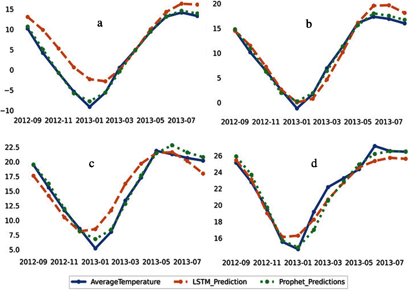
Figure 5: Performance of CDLSTM and FB-Prophet models for temperature forecasting using novel CDLSTM and FB-Prophet forecasted for (a) Jammu and Kashmir, (b) Himachal Pradesh, (c) Uttarakhand, (d) Nagaland Manipur Mizoram and Tripura

The FB-Prophet model implemented in the present investigation with the PWL algorithm showed remarkably efficient performance based on accuracy metrics, see Tabs. 3 and 4. As per available literature, the current investigation’s performance achieved by the FB-Prophet model for temperature and rainfall forecasting is the highest, based on accuracy metrics. The developed CDLSTM model has lower accuracy than the FB-Prophet model; however, the CDLSTM model showed better performance than models applied in previous studies. In the present investigation, the seasons in the Himalayan area were defined as per IMD and international standards. It is an important criterion to put the correct months as per the respective seasons. [4] defined summer as Jan and Feb, which might be an error. For India, the monsoon season overlaps with summer; therefore, studies focusing on rainfall trends and forecasting should use monsoon instead of summer rainfall to reduce ambiguity. Models based on ML require intense hyperparameter tuning to achieve performance with model stability. ML models might provide higher accuracy without proper optimization; however, this accuracy might be illusionary and unstable. The study was done by [4] to show a lack of hyperparameters tuning. The present investigation attempted rigorous hyperparameter optimization to ensure efficient model performance with model stability for the developed CDLSTM. Additionally, the CDLSTM model developed on temperature dataset was applied and assessed on a different dataset, i.e., rainfall dataset. In order to evaluate one model, it is imperative to conduct a comparative analysis with a different model for secular evaluation. The present investigation compared the developed CDLSTM model with the popular FB-Prophet model and showed significant performance; however, [4] did not compare the ANN model with another model. Data preprocessing steps such as removing missing values, data transformation, etc., are vital to building an efficient ML forecasting model. The study [4] observed that the rainfall data from 1901-2015 has no missing values; however, the present investigation found that the same dataset for the entire India had 1036 missing values. Therefore, the present investigation replaced the missing data values with the mean value of the respective parameter.

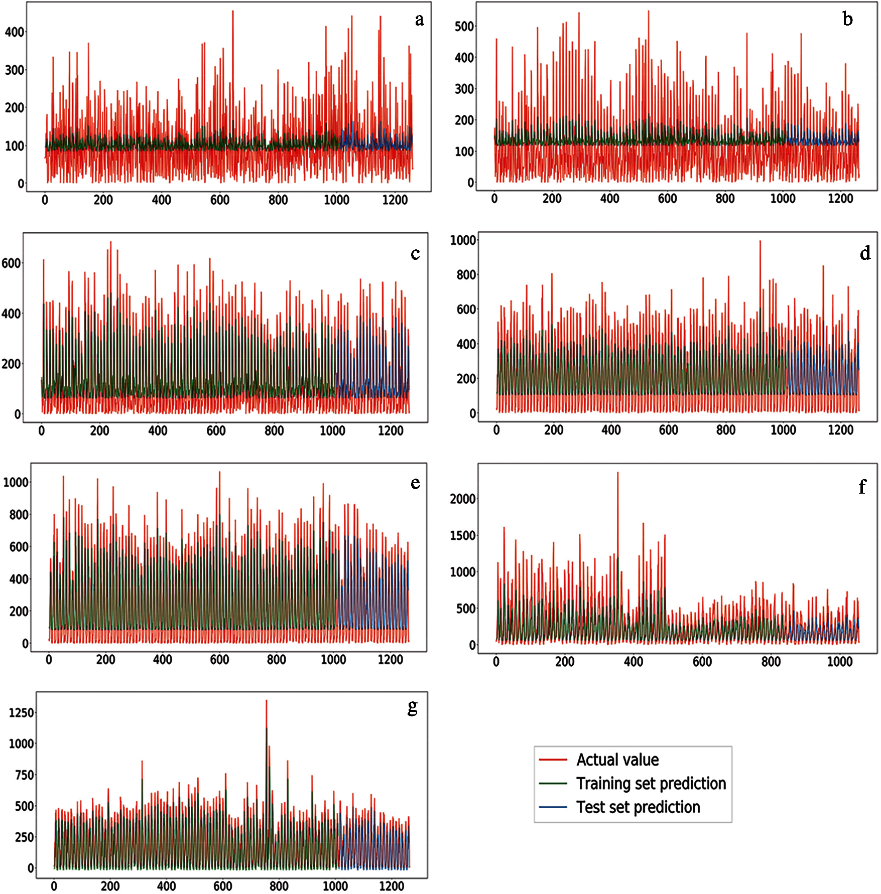
Figure 6: Performance of CDLSTM model for rainfall forecasting, training, and testing forecasted rainfall, shown using red, green, and blue, respectively

4.6 Computational Efficiency of the Present Investigation

After optimizing the CDLSTM model, it took 45 s 21 ms/step for 20 epochs, i.e., a total of 907 seconds or 15 min 12 sec to complete the training. Optimization saves computation cost by selecting the best number of parameters, including the number of epochs. The optimized model took only 40% computational time compared with 50 epochs in 40 minutes. The imported FB-Prophet model took three minutes to perform the results, only 20% of the computational processing time.

5  Conclusions

The present investigation provides an understanding of the long-term historical and forecasted data of temperature and rainfall for India’s Himalayan states. A DL-based LSTM model was developed based on rigorous hyper-parameters tuning to forecast the temperature and rainfall. The correlation coefficient, MSE, RMSE MAPE, NSE, and MAD were obtained to evaluate the CDLSTM model performance. All the twelve Himalayan states showed increasing temperatures after 2000 and a decrease in rainfall after 1990. Arun and NMMT showed decreasing trends for rainfall; however, rainfall over J&K, UK, WB&S showed an increasing trend. The Himalayan state with the highest average rainfall was Arun, while the lowest average rainfall was for J&K. Mean annual temperature of the Himalayan states increased around 1.07°C between the last two centuries; interestingly, it has increased 0.98°C for entire India for the same period. The Himalayan states are experiencing more severe impacts of global warming. The present investigation found a strong correlation (0.98) between the average temperature trend for all the Himalayan states. The correlation coefficient between temperature and rainfall was significantly strong for Northeastern Himalayan states A&M (0.80), WB&S (0.78), NMMT (0.76), and Arun (0.62); however, it was weak for Northwestern Himalayan states UK (0.5), Him (0.39) and J&K (0.18).

The present investigation developed the CDLSTM model containing eight LSTM layers, where four layers were dense, and three were the dropout layers. The CDLSTM model was optimized based on rigorous parameters tuning. The developed CDLSTM model showed promising performance based on various metrics such as R2, MSE, RMSE, MAPE, MAD, and NSE. The developed CDLSTM model was likely to estimate the possible future values of temperature and rainfall accurately, given its reliability. The FB-Prophet model implemented in the present investigation with the PWL algorithm showed remarkably efficient performance based on accuracy metrics. As per available literature, the current investigation’s performance achieved by the FB-Prophet model for temperature and rainfall forecasting is the highest, based on accuracy metrics. The developed CDLSTM model has lower accuracy than the FB-Prophet model; however, the CDLSTM model showed better performance than other models applied in previous studies. Both CDLSTM and FB-Prophet model’s performance showed good forecasting values for all months, including Jan 2013, where the temperature was low due to the peak winter season. The future scope of the present investigation is to add more data on snow retreat, glacier melt, agricultural yield, and demographics to assess the complete cycle of climate change for the Himalayan region. Another future scope of the present investigation is to implements and assimilate the latest state of the art models for climate modeling and forecasting [30–34].

6  Limitations and Learning Points of the Present Investigation

The significant limitations of the present study include (1) Although the performance of the developed CDLSTM model was significantly higher than previous studies, the imported FB-Prophet model with PWL algorithm performed better than the developed CDLSTM model. (2) The computation of the tuned CDLSTM model took 15 minutes for 20 epochs, so an improvement in computational efficiency is required. (3) The reasons to choose LSTM in the present investigation are its capability to deal with the vanishing gradient problem and better control, flexibility, and performance than traditional RNN. (4) The LSTM model has limitations such as the requirement of high memory bandwidth due to linear layers; also, it is more prone to overfitting and is too complex to apply dropout, (5) The effect of Gulfstream weakening on climate change on agricultural productivity will be a future scope as parts of the US and Europe are influenced by the Gulf Stream.

Acknowledgement: The author is thankful to IMD and the University of Berkeley for providing climate datasets.

Funding Statement: Mohd Anul Haq would like to thank Deanship of Scientific Research at Majmaah University for supporting this work under Project No. R-2021-236.

Conflicts of Interest: The author declare that they have no conflicts of interest to report regarding the present study.

References

 1.  P. Baral and M. A. Haq, “Spatial prediction of permafrost occurrence in Sikkim Himalayas using logistic regression, random forests, support vector machines and neural networks,” Geomorphology, vol. 371, no. July, pp. 107331, 2020. [Google Scholar]

 2.  M. A. Haq, M. Alshehri, G. Rahaman, A. Ghosh, P. Baral et al., “Snow and glacial feature identification using hyperion dataset and machine learning algorithms,” Arabian Journal of Geosciences, vol. 14, no. 15, pp. 1–21, 2021. [Google Scholar]

 3.  M. A. Haq, K. Jain and K. P. R. Menon, “Modelling of Gangotri glacier thickness and volume using an artificial neural network,” Int. Journal of Remote Sensing, vol. 35, no. 16, pp. 6035–6042, 2014. [Google Scholar]

 4.  B. Praveen, S. Talukdar, Shahfahad, S. Mahato, J. Mondal et al., “Analyzing trend and forecasting of rainfall changes in India using non-parametrical and machine learning approaches,” Scientific Reports, vol. 10, no. 1, pp. 1–21, 2020. [Google Scholar]

 5.  S. Nandargi, A. Gaur and S. S. Mulye, “Hydrological analysis of extreme rainfall events and severe rainstorms over Uttarakhand, India,” Journal of Hydrological Science, vol. 61, no. 12, pp. 2145–2163, 2016. [Google Scholar]

 6.  R. Venkata Ramana, B. Krishna, S. R. Kumar and N. G. Pandey, “Monthly rainfall prediction using wavelet neural network analysis,” Water Resources Management, vol. 27, no. 10, pp. 3697–3711, 2013. [Google Scholar]

 7.  M. Shenify, A. S. Danesh, M. Gocić, R. S. Taher, A. W. A. Wahab et al., “Precipitation estimation using support vector machine with discrete wavelet transform,” Water Resources Management, vol. 30, no. 2, pp. 641–652, 2016. [Google Scholar]

 8.  F. Kratzert, D. Klotz, C. Brenner, K. Schulz and M. Herrnegger, “Rainfall-runoff modelling using long short-term memory (LSTM) networks,” Hydrology and Earth System Sciences, vol. 22, no. 11, pp. 6005–6022, 2018. [Google Scholar]

 9.  J. Kuttippurath, S. Murasingh, P. A. Stott, B. B. Sarojini, M. K. Jha et al., “Observed rainfall changes in the past century (1901-2019) over the wettest place on Earth,” Environmental Research Letters, vol. 16, no. 2, pp. 1–14, 2021. [Google Scholar]

10. L. Tamiotti, R. Teh, V. Kulaçoglu, A. Olhoff, B. Simmons et al., “Climate change: The current state of knowledge,” Trade and Climate Change, vol. 9177, no. June, pp. 1–46, 2009. [Google Scholar]

11. M. A. Haq, P. Baral, S. Yaragal and G. Rahaman, “Assessment of trends of land surface vegetation distribution, snow cover and temperature over entire Himachal Pradesh using MODIS datasets,” Natural Resource Modeling, vol. 33, no. 2, pp. 941, 2020. [Google Scholar]

12. S. Singh, M. Kaushik, A. Gupta and A. K. Malviya, “Weather forecasting using machine learning techniques,” SSRN Electronic Journal, vol. 2, no. June, pp. 1–6, 2019. [Google Scholar]

13. A. Basistha, D. S. Arya and N. K. Goel, “Analysis of historical changes in rainfall in the Indian Himalayas,” International Journal of Climatology, vol. 29, no. 4, pp. 555–572, 2009. [Google Scholar]

14. V. Kumar, S. K. Jain and Y. Singh, “Analyse des tendances pluviométriques de long terme en Inde,” Hydrological Sciences Journal, vol. 55, no. 4, pp. 484–496, 2010. [Google Scholar]

15. A. Banerjee, A. P. Dimri and K. Kumar, “Rainfall over the Himalayan foot-hill region: Present and future,” Journal of Earth System Science, vol. 129, no. 1, pp. 39, 2020. [Google Scholar]

16. A. Banerjee, A. P. Dimri and K. Kumar, “Temperature over the Himalayan foothill state of Uttarakhand: Present and future,” Journal of Earth System Science, vol. 130, no. 1, pp. 1–14, 2021. [Google Scholar]

17. K. Greff, R. K. Srivastava, J. Koutnik, B. R. Steunebrink, J. Schmidhuber et al., “LSTM: A search space odyssey,” IEEE Transactions on Neural Networks and Learning Systems, vol. 28, no. 10, pp. 2222–2232, 2017. [Google Scholar]

18. B. Yan, J. Wang, Z. Zhang, X. Tang, Y. Zhou et al., “An improved method for the fitting and prediction of the number of COVID-19 confirmed cases based on LSTM,” Computers, Materials & Continua, vol. 64, no. 3, pp. 1473–1490, 2020. [Google Scholar]

19. J. Zhao, J. Wu, X. Guo, J. Han, K. Yang et al., “Prediction of radar sea clutter based on LSTM,” Journal of Ambient Intelligence and Humanized Computing, vol. 2004, no. 1, pp. 9, 2019. [Google Scholar]

20. C. Hu, Q. Wu, H. Li, S. Jian, N. Li et al., “Deep learning with a long short-term memory networks approach for rainfall-runoff simulation,” Water, vol. 10, no. 11, pp. 1543, 2018. [Google Scholar]

21. K. Fang and C. Shen, “Near-real-time forecast of satellite-based soil moisture using long short-term memory with an adaptive data integration kernel,” Journal of Hydrometeorology, vol. 21, no. 3, pp. 399–413, 2020. [Google Scholar]

22. H. B. Mann, “Nonparametric tests against trend,” Econometrica, vol. 13, no. 3, pp. 245, 1945. [Google Scholar]

23. M. Kendall, “Rank correlation methods,” Griffin, London, 1970. [Google Scholar]

24. P. K. Sen, “Estimates of the regression coefficient based on Kendall’s tau,” Journal of the American Statistical Association, vol. 63, no. 324, pp. 1379–1389, 1968. [Google Scholar]

25. R. Schumacker, S. Tomek, R. Schumacker and S. Tomek, “z-Test,” in Understanding Statistics Using R, NY, USA, 2013. [Google Scholar]

26. A. Jabeen, S. Afzal, M. Maqsood, I. Mehmood, S. Yasmin et al., “An LSTM based forecasting for major stock sectors using COVID sentiment,” Computers, Materials & Continua, vol. 67, no. 1, pp. 1191–1206, 2021. [Google Scholar]

27. O. A. Fallatah, M. Ahmed, D. Cardace, T. Boving and A. S. Akanda, “Assessment of modern recharge to arid region aquifers using an integrated geophysical, geochemical, and remote sensing approach,” Journal of Hydrology, vol. 569, no. 1, pp. 600–611, 2019. [Google Scholar]

28. A. Qian, S. Yi, L. Chang, G. Sun and X. Liu, “Using grace data to study the impact of snow and rainfall on terrestrial water storage in Northeast China,” Remote Sensing, vol. 12, no. 24, pp. 1–21, 2020. [Google Scholar]

29. M. Chhetri, S. Kumar, P. P. Roy and B. G. Kim, “Deep BLSTM-GRU model for monthly rainfall prediction: A case study of Simtokha, Bhutan,” Remote Sensing, vol. 12, no. 19, pp. 1–13, 2020. [Google Scholar]

30. E. S. M. E. Kenawy, S. Mirjalili, S. M. S. Ghoneim, M. M. Eid, M. Marwa et al., “Advanced ensemble model for solar radiation forecasting using sine cosine algorithm and Newton’s laws,” IEEE Access, vol. 9, pp. 115750–115765, 2021. [Google Scholar]

31. S. S. M. Ghoneim, T. A. Farrag, A. A. Rashed, E. S. M. E. Kenawy and A. Ibrahim, “Adaptive dynamic meta-heuristics for feature selection and classification in diagnostic accuracy of transformer faults,” IEEE Access, vol. 9, pp. 78324–78340, 2021. [Google Scholar]

32. A. A. Salamai, E. S. M. E. Kenawy and I. Abdelhameed, “Dynamic voting classifier for risk identification in supply chain 4. 0,” CMC-Computers, Materials & Continua, vol. 69, no. 3, pp. 3749–3766, 2021. [Google Scholar]

33. E. S. M. E. Kenawy, H. F. Abutarboush, A. W. Mohamed and A. Ibrahim, “Advance artificial intelligence technique for designing double t-shaped monopole antenna,” CMC-Computers, Materials & Continua, vol. 69, no. 3, pp. 2983–2995, 2021. [Google Scholar]

34. M. A. Haq, M. F. Azam and C. Vincent, “Efficiency of artificial neural networks for glacier ice-thickness estimation: A case study in western Himalaya, India,” Journal of Glaciology, vol. 67, no. 264, pp. 671–684, 2021. [Google Scholar]

This work is licensed under a Creative Commons Attribution 4.0 International License, which permits unrestricted use, distribution, and reproduction in any medium, provided the original work is properly cited.