Computers, Materials & Continua DOI:10.32604/cmc.2022.023086
Article

Analysis and Modeling of Propagation in Tunnel at 3.7 and 28 GHz

Md Abdus Samad1,2 and Dong-You Choi1,*

1Department of Information and Communication Engineering, Chosun University, Gwangju, 61452, Korea
2Department of Electronics and Telecommunication Engineering, International Islamic University Chittagong, Chittagong, 4318, Bangladesh
*Corresponding Author: Dong-You Choi. Email: dychoi@chosun.ac.kr
Received: 27 August 2021; Accepted: 15 October 2021

Abstract: In present-day society, train tunnels are extensively used as a means of transportation. Therefore, to ensure safety, streamlined train operations, and uninterrupted internet access inside train tunnels, reliable wave propagation modeling is required. We have experimented and measured wave propagation models in a 1674 m long straight train tunnel in South Korea. The measured path loss and the received signal strength were modeled with the Close-In (CI), Floating intercept (FI), CI model with a frequency-weighted path loss exponent (CIF), and alpha-beta-gamma (ABG) models, where the model parameters were determined using minimum mean square error (MMSE) methods. The measured and the CI, FI, CIF, and ABG model-derived path loss was plotted in graphs, and the model closest to the measured path loss was identified through investigation. Based on the measured results, it was observed that every model had a comparatively lower (n < 2) path loss exponent (PLE) inside the tunnel. We also determined the path loss component's possible deviation (shadow factor) through a Gaussian distribution considering zero mean and standard deviation calculations of random error variables. The FI model outperformed all the examined models as it yielded a path loss closer to the measured datasets, as well as a minimum standard deviation of the shadow factor.

Keywords: Path loss; shadow factor; telecommunications; train tunnel; wave propagation; wireless networks

1  Introduction

With the rapidly increasing pace of human lives, there has been an increase in the widespread usage of tunnels for a variety of purposes, such as transportation, mining of fossil fuels, minerals, and military operations. Among these types of tunnels, train tunnels play an essential role in present day life. Consequently, deploying a 5G network inside a tunnel is critical to ensure security and safety, and to increase the efficiency of train operations [1]. Reliable transmission is required to achieve a stable and efficient telecommunication facility between the transmitter and receiver. Path loss is an essential component that may be adversely affected by several elements, such as signal frequency, distance from source to destination, environmental conditions, effect of signal fading and weather conditions [2]. Numerous models of various propagation pathway losses for multiple interferences and noise-limited settings have been investigated in myriad ways to address the random characteristic of wireless networks [3].

Nevertheless, knowledge of radio propagation inside a tunnel is essential for setting up the transmitter and receiver and to actualize the system specifications. For instance, statistical features on the wireless channel are significant in defining transmitter and receiver characteristics and in budget link computation, such as the probability density function of the received signal intensity and fade durations. In addition, the current radio propagation models typically predict the path loss, power delay profile, or delay spread for specific transmitter and receiver locations [4]. However, it is generally accepted that the propagation inside a tunnel is distinctly different when compared to other types of propagation media, such as outdoor, outdoor to indoor, indoor to outdoor, or indoor-to-indoor radio wave propagation [5]. The fundamental difference in the tunnel is that the radio wave is enclosed by the blocking surface (of the tunnel) through which the refracted wave cannot reach the receiver, and as such a propagated signal is received in other cases through a penetration loss at the tunnel blocking plane. Therefore, the propagation of radio waves inside the tunnel must be investigated independently.

The properties of the wireless propagation channel determine the ultimate performance of a wireless telecommunication network based on the required quality of service (QoS). Consequently, a realistic understanding of wireless propagation channels in a tunnel environment is essential. To date, several studies on communication channels have been conducted in various tunnels [6–8]. In contrast to open-air propagation, tunnel propagation includes electromagnetic waves in an enclosed environment [9]. A leaky feeder communication system can be deployed inside confined locations, in particular inside road or rail tunnels [5]. The cable is leaky in the sense that it includes gaps or slots in its outer conductor that allow radio signals to leak into or out of the cable along its entire length. As a result of such signal loss, line amplifiers must be installed at regular intervals to boost the signal back to acceptable levels that results in significant weight and cost increases [10]. However, there is a high probability that the cable can be damaged inside the tunnel, resulting in communication complications in the entire tunnel. Consequently, leaky feeders are not generally deployed inside tunnels for telecommunication purposes.

Currently, modal expansion in tunnels or corridors is used as a standard approach in wave propagation analysis [4,11–13]. Given that a tunnel is considered an empty waveguide, the modal expansion technique can be applied to determine wave propagation. The cross-section of the tunnel can be represented as the sum of the transverse eigenmodes above the cutoff frequency. However, this technique becomes ineffective at high frequencies, such as the millimeter wavelength where the dimensions of the transverse wavelength are far broader, and numerous modes need to be considered.

Radio-wave propagation modeling inside a tunnel can be performed using electromagnetic waves by numerical methods. However, the numerical approach of finding radio wave propagation inside a tunnel is complex and requires large computing capacity. Consequently, several simplified techniques to reduce the computational complexity were proposed in subsequent studies: namely the finite difference time domain (FDTD) [14], Crank Nicolson (CN) method [15], vector parabolic equation (VPE) [16,17], scalar parabolic equation (SPE) [17], and uniform theory of diffraction (UTD) [18–20]. Nevertheless, all these simplified techniques are hindered by certain impediments such as: the usage of the FDTD method is limited to the large-sized tunnel, the CN entails the resolution of sets of simultaneous equations that might become large enough that dense mesh issues cannot be addressed efficiently, the VPE technique assumes that fields travel within 30° in the propagation direction, the SPE can only be used for tunnels with perfect electrical conductor (PEC) walls, and UTD cannot be used at the junctions where tunnels do not cross perpendicularly.

A widely-accepted path loss model can be implemented in a tunnel using the ray-tracing technique (RT). However, this technique has several limitations in the implementation and analysis of RT signals. For example, an implementation through delay line time-domain analysis is minimal if the minimum delay is less than 8 ns (in which case, it will require a larger bandwidth (BW); for instance, a 1 ns time delay will require 1 GHz BW) [21]. While an alternative implementation utilizes the shooting and bouncing RT realization technique, this approach has the impediment of the hypothetical size of the receiver receiving the propagated ray [22,23]. Another implementation of RT is through 3D ray-tracing modeling, which has to deal with the challenge of obtaining convergence results as there are numerous reflections [24].

Consequently, modal expansion, numerical approach, and RT-based techniques of wave propagation in tunnels have significant challenges. Conversely, a large-scale path loss model was employed for model wave propagation in the tunnel [25], and the results indicate that large-scale path loss models could be effective at modelling radio wave propagation inside tunnels. Moreover, large-scale path loss models have been used to model indoor corridors [26,27] and stairwells [28]. Therefore, we used large-scale path loss models to model the measured data, and found that the results were satisfactory. This study makes the following contributions:

•   We examined the wave propagation in the newly built train tunnel, called Mangyang Tunnel 2, in South Korea, and the measured path loss was modeled using the CI, FI, CIF, and ABG models.

•   The path loss parameters of the CI, FI, CIF, and ABG models were calculated using the MMSE optimization technique.

•   We analyzed the free space path loss (FSPL) and PLE variations of the CI, FI, CIF, and ABG models over 3.7 to 28 GHz frequency bands.

•   We also modeled the shadow factor using the Gaussian distribution of the studied path loss models.

The remainder of this paper is organized as follows: Section 2 provides experimental scenarios and experimental parameter descriptions. Section 3 provides analytical models of CI, FI, CIF, and ABG models and MMSE-derived optimized parameter calculation procedures. Section 4 discusses the outcomes obtained from the experimental results. Finally, the conclusions are presented in Section 5.

2  Measurement Experiment

This section describes the measurement technique, soundings, and instruments used for the experiment, as well as characterizing the equipment used at the transmitter and receiver ends.

2.1 Measuring Tools

This section includes the detailed description of the channel sounder and the scenarios covered in this measurement experiment. The basic architecture of the experimental scenario is illustrated in Fig. 1. We utilized the M5183B keysight signal generator at the transmitter end and the keysight PXI 9393A signal analyzer at the receiver end. The MXG N5183B signal generator can transmit continuous wave (CW) signals at 9–40 GHz. The PXI 9393A signal analyzer used as the receiver has a frequency range of 9–30 GHz. Guided horn antennas at the frequency of 3.5 GHz (directional antenna horn), 28 GHz (directional antenna horn), and 28 GHz tracking antenna system (TAS) were used in the experiment, where the antenna gain was 10, 20, and 20 dBi, respectively. The guided horn antennas were assembled with horizontal-horizontal co-polarization. The specific computing operational parameters are listed in Tab. 1. High-frequency bands from RF to microwave frequency can be generated using the analog signal generator MXG N5183B [29]. Analog signal generation offers the possibility of adding amplitude, frequency, phase, and pulse modulation to the (CW) transmissions from the transmitter. Moreover, frequency changeover can be performed using a listing mode with a switching time of 600 μs. In the sweep mode, the lists change step by step, similar to frequency switching. The system can produce a low power of approximately—−130 dBm and a maximum power of approximately +20 dBm. The level of accuracy of the signal generator is approximately ± 0.7 dB (at 10 GHz), and at 1 GHz with a 20 kHz offset, the single-sideband modulation phase noise of the device is –124 dBc/Hz. In the range of 0.5–64 rad, the signal generator may produce a pulse width of 10 ns and pulse modulation phase deviation in the normal mode. The frequency range of 9 kHz to 9, 4, 14, 18, or 27 GHz was analyzed with this instrument in an extended mode from 3, 6 —50 GHz. The absolute amplitude accuracy was ± 0.13 dB, and the frequency switching was approximately smaller than 135 μs. The intermodulation of the 3rd order was approximately +31 dBm, and the device showed a medium noise level of up to −168 dBm/Hz.

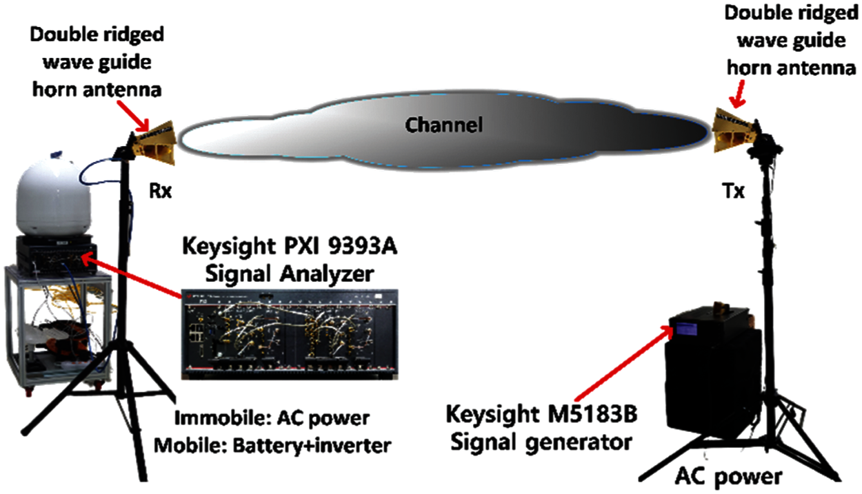
Figure 1: Channel sounder architecture

2.2 Experiment Description

The measurement experiment site is Mangyang Tunnel 2, located in Mangyang-ri, Giseong-myeon, Uljin-gun, Gyeongsangbuk-do, South Korea. The newly built tunnel, Mangyang Tunnel 2, is used for transportation by trains. The experiments were conducted in the tunnel before its opening, and consequently, safety issues were easily ensured. Some of the measurement attempts are presented in Figs. 2a–2b. All the equipment and technical support during the measurement experiment was provided by TA Engineering Inc., South Korea. The organization deployed a physical transmitter and receiver, a mobile trolley, and other experimental facilities. Mechanical adjustments allow the transmitter's antenna to be physically modified. The tunnel geometry at the entrance (of the experiment starting point) and some of the irregularities in the tunnel structure are shown in Figs. 2c–2d. The receiver unit was installed on a trolley, which was specially designed for experimental purposes. The transmitter's horn antenna was directed toward the central receiver unit, while the receiver trolley was moved inside the tunnel at regular intervals of 10 m up to 1500 m and then at regular intervals of 20 m for the rest of the path, and the received signal strength was measured. Thus, the received signal was measured at a total of 160 places.

2.3 Data Pre-Processing

Path loss is crucial in radio channel models to design the link budget and coverage of wireless networks. The path loss of a radio link can be calculated as:

PL=PTx−PRx+GTx+GRx−CTx−CRx(1)

where PTx is the transmitted signal power, PRx is the received signal power, GTx and GRx are the gains of the used antennas, and CTx, CRx are the cable losses at the Tx and Rx ends, respectively. We measured the received power, and the other gain-related parameters were calculated from the system specifications and datasheets.

3  Path Loss Prediction Models

Absorption and scattering are two primary processes in large-scale signal attenuation. Typically, path loss and shadowing are used to describe the large-scale signal attenuation. The relationship between path loss and channel distance is typically characterized by two models: single-frequency model and multi-frequency model, based on empirical data acquired from channel measurements. The large-scale CI, FI, CIF, and ABG models have a fixed mathematical structure, and certain parameters whose values change according to operational frequency, terrain setting, and environmental factors. This section determines the propagation parameters using the CI, FI, CIF, and ABG models, which are discussed in detail in the following subsections.

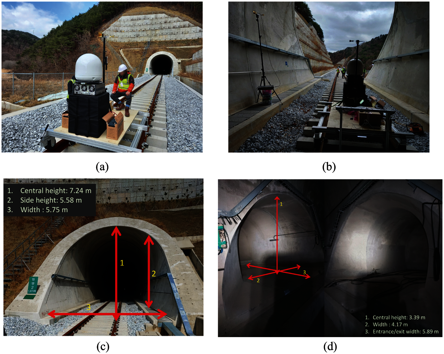
Figure 2: (a) Receiver movement trolley on the train rail, (b) Transmitter and the receiver together at an initial measurement, (c) Tunnel geometry at the entrance on one side, and (d) Structural changes in the tunnel: change in tunnel structure at the points 220, 770, 1000, 1260, 1500 m

3.1 Single Frequency Propagation

3.1.1 Close-In (CI) Model

The Equation for the CI model of wave propagation is:

PLCI(f,d)=L(f,1m)+10nlog10(d)+Sμ,σCI[dB]ford≥1m(2)

where S is a Gaussian random variable, which means that the random variable can be expressed through the mean (μ) and standard deviation σ in dB, where the mean (μ) is zero, but the standard deviation (σ) is a non-zero value. The random variable S shows large-scale channel variations within a limit (defined by the probability density function) as a result of the shadowing effect [30]. The free space path loss L(f,1m) is given by 10log10(4πf/c)2 for a distance of 1 m, and n is the PLE. The PLE (n) path loss pattern is determined by the MMSE method that equals the value determined to the minimum mean square error (by reducing σ) with the original physical anchor point, realized by the free space power transmitted by the transmitting antenna [31]. To determine the optimum PLE where the path loss is minimum, Eq. (2) can be rearranged using the MMSE method as

Sμ,σCI=PLCI(f,d)[dB]−L(f,1m)−10nlog10(d)ford≥1m(3)

Assuming F=PLCI(f,d)[dB]−L(f,1m), and Z=10log10(d), then the Eq. (2) can written as:

Sμ,σCI=F−nZ(4)

The standard deviation of the shadow factor can be determined as:

σCI=Σ(Sμ,σCI)2/Σ(Sμ,σCI)2NN=∑(F−nZ)2/∑(F−nZ)2NN(5)

where N is the number of Tx-Rx separation distances. Minimizing the shadow factor with standard deviation σCI is commensurate to reducing the term ∑(F−nZ)2. If ∑(F−nZ)2 is reduced, the derivative of n should be zero:

d∑(F−nZ)2/d∑(F−nZ)2dndn=∑2Z(nZ−F)=2∑Z(nZ−F)=2(n∑Z2−∑ZF)=0(6)

Therefore, from Eq. (6):

n=∑FZ/∑FZ∑Z2∑Z2(7)

Consequently, the lowest standard deviation for the CI model is

σminCI=∑(F−nZ)2/∑(F−nZ)2NN(8)

The calculated values of n for the CI model are listed in Tab. 2.

3.1.2 Floating-Intercept (FI) Model

The FI path loss model is expressed by:

PLFI(d)[dB]=α+10⋅βlog10(d)+Sμ,σFI(9)

where α is the floating-intercept in dB, which is equivalent to the free space path loss, and β is the slope of the path loss vs. frequency line, which is comparable to the PLE as calculated in the CI model. The term S is a Gaussian random variable with zero mean and standard deviation σCI, defining large-scale signal variations. This method is also utilized in WINNER II [32] and 3GPP standards [33]. Remarkably, Eq. (9) requires two parameters, whereas the CI method requires only a single parameter, PLE (n). Assuming, F=PLFI(d)[dB], and Z=10log10(d) the minimum shadow factor can be determined using Eq. (10).

Sμ,σFI=F−α−βZ(10)

and the SF standard deviation is:

σFI=∑(Sμ,σFI)2/N=∑(G−α−βZ)2/N(11)

The minimum standard deviation σFI was determined based on the minimum value of the term ∑(G−α−βZ)2/N. As the term N is a constant number, it needs to minimize ∑(F−α−βZ)2 and, the same can be achieved by finding the derivative with respect to α and β as follows:

∂∑(F−α−βZ)2/∂∑(F−α−βZ)2∂α∂α=∑2(α+βZ−F)=2(Nα+β∑Z−∑F)=0(12)

∂∑(F−α−βZ)2/∂∑(F−α−βZ)2∂β∂β=∑2Z(α+βZ−F)=2(α∑Z+β∑Z2−∑ZF)=0(13)

Eqs. (12) and (13) yield:

Nα+β∑Z−∑F=0(14)

α∑Z+β∑Z2−∑ZF=0(15)

Combining (14) and (15), we get:

α=(∑Z∑ZF−∑Z2∑F)/(∑Z∑ZF−∑Z2∑F)[(∑Z)2−N∑Z2][(∑Z)2−N∑Z2](16)

β=(∑Z∑F−N∑ZF)/(∑Z∑F−N∑ZF)[(∑Z)2−N∑Z2][(∑Z)2−N∑Z2](17)

The optimum standard deviation of SF can be achieved by replacing α and β in Eq. (11) with Eqs. (16) and (17), respectively. The mean values of all vector elements were determined directly in the dB scale. The calculated values of the term n for the FI model are listed in Tab. 2.

3.2 Multi-Frequency Propagation

3.2.1 CIF Model

In [3], a multi-frequency method was considered adequate in a closed indoor environment, as frequency-dependent loss occurs after a distance of 1 m from the transmitter owing to the surrounding environment. The CI model can be adapted to implement the frequency-dependent path loss exponent (CIF) that utilizes the same physically driven free space path loss anchor at 1 m as the CI model. The path loss of the CIF method is calculated by:

PLCIF(f,d)[dB]=L(f,1m)+(n(1−n)+nbf/nbff0f0)10⋅log⁡(d/d1m1m)+Sμ,σCIF(18)

where d(m) is the distance between Tx and Rx greater than 1 m, n is the path loss exponent (PLE) that describes the dependence of propagation loss in the path (in dB) to the logarithm of the distance starting at 1 m, and S is the Gaussian random variable with zero mean and standard deviation σ(dB). This random variable characterizes the large-scale channel fluctuations due to shadowing, and b is an optimization parameter that presents the path loss slope of the linear frequency dependence. The term L(f,1m) is the free-space loss at a distance of 1 m, with fc being the center frequency L(dB)=32.4+20log⁡fc(GHz). The symbol f(GHz) is the operating carrier frequency and f0, as the minimum investigated, is the frequency of operating frequencies [34]. The frequency f0 is computed as follows:

f0=∑k=1KfkNk/∑k=1KfkNk∑k=1KNk∑k=1KNk(19)

where f0 is the weighted frequency average of all measurements for each particular scene, that is determined by considering the product of the sum of all the frequencies, the total number of recorded data Nk at a specific frequency and antenna scenario, and the corresponding frequency fk, and dividing that by the total number of measurements (that is, the summation of Nk from k=1 to K) taken over all frequencies for that specific scenario and the used transmitter and receiver system.

CIF method: MMSE-based parameters

After changing the side of Eq. (18), if we assume that F=PLCIF(f,d)[dB]−L(f,d0), Z=10log⁡(d/d1m1m), p=n(1−b), and q=nb/nbf0f0, we obtain

Sμ,σCIF=F−Z(p+qf)(20)

The shadow factors’ standard deviation is:

σCIF=∑(Sμ,σCIF)2/N=∑[F−Z(p+qf)]2/N(21)

Minimizing σCIF is equivalent to minimizing ∑[F−Z(p+qf)]2. When ∑[F−Z(p+qf)]2 is minimized, its derivatives with respect to p and q should be zero, i.e.,

∂∑[F−Z(p+qf)]2/∂∑[F−Z(p+qf)]2∂p∂p=∑2Z(pZ+qZf−F)=2(p∑Z2+q∑Z2f−∑ZF)=0(22)

∂∑[F−Z(p+qf)]2/∂∑[F−Z(p+qf)]2∂q∂q=∑2Zf(pZ+qZf−F)=2(p∑Z2f+q∑Z2f2−∑ZFf)=0(23)

After simplification and combining, we obtain:

p=(∑Z2f∑ZFf−∑Z2f2∑ZF)/(∑Z2f∑ZFf−∑Z2f2∑ZF)[(∑Z2f)2−∑Z2∑Z2f2][(∑Z2f)2−∑Z2∑Z2f2](24)

q=(∑Z2f∑ZF−∑Z2∑ZFf)/(∑Z2f∑ZF−∑Z2∑ZFf)[(∑Z2f)2−∑Z2∑Z2f2][(∑Z2f)2−∑Z2∑Z2f2](25)

In Eqs. (24) and (25), the closed-loop solution of the assumed terms p and q was derived. The standard derivation of the shadow factor can be derived by inserting p and q into Eq. (21). Moreover, by using the initial definition, p=n(1−b) and q=nb/nbf0f0 the values of n and b can be calculated. The calculated values of the CIF model are listed in Tab. 2.

3.2.2 Alpha-Beta-Gamma (ABG) Model

A multi-frequency three-component model called the ABG model contains conditions for describing the propagated loss at different frequencies depending on the frequency and distance [31,34]. The path loss of the ABG model is given by Eq. (26):

PLABG(f,d)[dB]=10αlog10(d/d1m1m)+β+10γlog10(f/f1GHz1GHz)+Sμ,σABG(26)

where α and γ are associated with the path length and frequency element of path loss of the link, f is the frequency in GHz, and β is a parameter utilized as an offset mechanism that does not have any physical meaning. The parameter S is a Gaussian random variable representing large-scale signal variations in the mean path loss over distance. The ABG model can be recognized as the annex of the FI model for multiple frequencies. The MMSE technique can be used to determine the optimum values of the α, β, and γ coefficients. It can be shown that if γ= 0 or 2 and the ABG model is used for a single frequency, it transforms into an FI model. As a result, the ABG model is a multi-frequency generalization of the FI, and the FI can also be constructed using a single frequency [35]. In addition, the ABG model may be simplified to the CI, if α equals 20log(4pi/c), β equals PLE, and γ equals 2. Given that the ABG model requires three parameters whereas the CI model requires just one parameter, the CI model is more economical in computing complexity. Moreover, others argue that the additional two variables in the ABG model provide only a marginal improvement in accuracy [36,37]. The MMSE-based minimum parameter values can be determined by assuming F=PLABG(f,d)[dB], Z=10log10(d) and P=10log10(f) in Eq. (26), then SF is calculated by

Sμ,σABG=F−αZ−β−γP(27)

and the SF standard deviation is:

σABG=∑(Sμ,σABG)2/N=∑(F−αZ−β−γP)2/N(28)

To obtain the minimum values of the standard deviation from Eq. (28), ∑(F−αZ−β−γP)2/N needs to be minimized. Given that N is a constant, to minimize the ∑(F−αZ−β−γP)2, its partial derivative with respect to α, β, and γ should be zero.

∂∑(F−αZ−β−γP)2/∂∑(F−αZ−β−γP)2∂α∂α=∑2Z(αZ+β+γP−F)=2(α∑Z2+β∑Z+γ∑ZP−∑ZF)=0(29)

∂∑(F−αZ−β−γP)2/∂∑(F−αZ−β−γP)2∂β∂β=∑2(αZ+β+γP−F)=2(α∑Z+Nβ+γ∑P−∑F)=0(30)

∂∑(F−αZ−β−γP)2/∂∑(F−αZ−β−γP)2∂γ∂γ=∑2P(αZ+β+γP−F)=2(α∑ZP+β∑P+γ∑P2−∑PF)=0(31)

From Eqs. (29)–(31), it is clear that

α∑Z2+β∑Z+γ∑ZP−∑ZF=0(32)

α∑Z+Nβ+γ∑P−∑F=0(33)

α∑ZP+β∑P+γ∑P2−∑P=0(34)

The numeric values of α, β, and γ for the ABG model can be calculated by solving Eq. (35), and the calculated coefficients of the ABG model are given in Tab. 2.

(αβγ)=(∑Z2∑Z∑ZP∑ZN∑P∑ZP∑P∑P2)−1(∑ZF∑F∑PF)(35)

4  Results and Discussions

4.1 Analysis of the Large-Scale Path Loss Models

Measurement experiments at 3.7 and 28 GHz were conducted to examine the parameters of long-term path loss models in a train tunnel. The transmitting antenna was directed inwards, and the receiver, located in the middle of the mobile van, was directed toward the receiving antenna. As mentioned earlier, three different channels were created at two frequencies (3.7 and 28 GHz) using horn and TAS antennas. We processed our measured data and produced the visible figures with MATLAB R2021a. Fig. 3 depicts the coefficients of the models with diverse FSPL and PLE values.

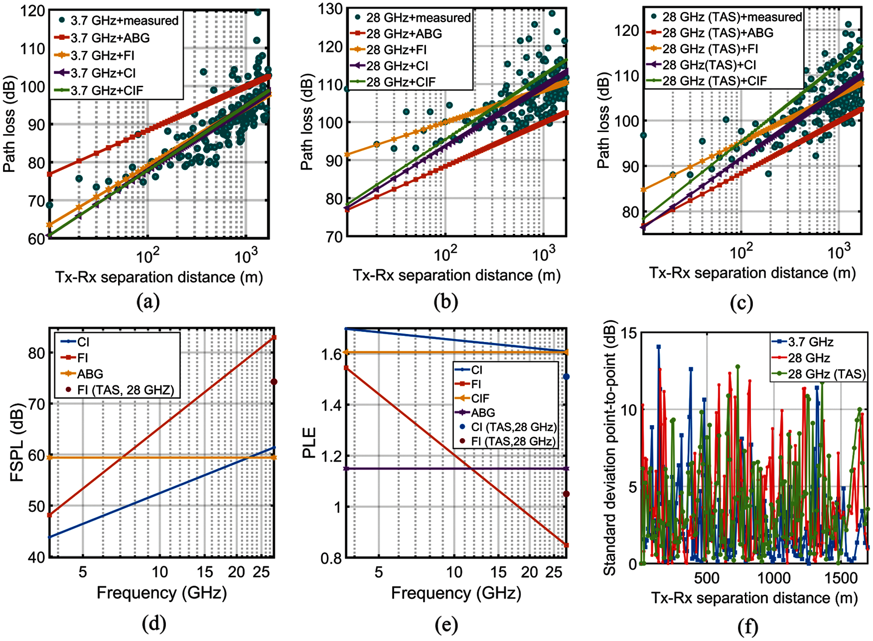
Figure 3: CI, CIF, FI, ABG model, and measured path loss in the tunnel at (a) 3.7 GHz, (b) 28 GHz, (c) 28 GHz (TAS); (d) FSPL variations at different frequencies developed by CI, FI, CIF, and ABG models, (e) PLE variations at different frequencies developed by CI, FI, CIF, and ABG models, (f) Standard deviation of point-to-point variations of received power

Fig. 3a shows the changes in path loss in the 1674 m long straight train tunnel on a semi-log scale. A scatter plot was used to depict the measured path losses at various points. The recorded path loss was fitted using the CI, FI, CIF, and ABG models, all plotted as straight lines. As shown in Fig. 3a, the ABG model did not fit well with the measured datasets. Except for the ABG model, the other models, CI, FI, and CIF, are competitive when considering the prediction performance. Additionally, CI, FI, and CIF models show almost identical path loss predictions at the far end, but a variation appears at the near end for FI models when compared to the CI and CIF models. At the near end, the FI model fitted the measured data in contrast to the CI and CIF models. Consequently, at 3.7 GHz frequency, the FI model fitted the measured dataset with greater efficiency than the other models.

Fig. 3b shows the changes in path loss in the 1674 m long straight train tunnel on a semi-log scale at a frequency of 28 GHz. While both the CI and CIF models showed good performance at the far end of the tunnel, they did not perform well at the near end. At a frequency of 28 GHz, the ABG model did not fit well with the measured dataset, where the ABG model parameters were calculated using the MMSE-based optimization technique. Of the remaining models, the FI model fitted the measured dataset with greater efficiency than the CI and CIF models at 28 GHz.

Fig. 3c shows the changes in path loss in the 1674 m long straight train tunnel on a semi-log scale at a frequency of 28 GHz. The figure shows that the FI model performs well at the 28 GHz TAS receiver when compared to the CI, CIF, and ABG models. At 28 GHz frequency with the TAS receiver, the ABG model did not fit well with the measured dataset. The path loss predicted by the FI model fits well with the measured datasets, and shows higher accuracy at both the near and far ends.

4.2 FSPL Variations in Different Propagation Techniques

Fig. 3d shows the variations in FSPL exhibited by the CI, FI, CIF, and ABG models. As the FSPL of the CI and CIF models is the same, for brevity the CIF model is not depicted in the figure. The FSPL developed by the ABG model is a constant quantity, as depicted by the straight yellow line marked by a hexagonal-shaped marker. While the FSPL of the CI model is much lower than that of the other models, it is evident in Figs. 3a–3c that the CI model did not outperform the FI model at the frequencies of 3.7, 28, and 28 (TAS) GHz. The FSPL at 28 GHz with the TAS receiver is a different value, as depicted in the figure by a single red scatter point. Consequently, it is clear that the FI model has a positive slope of FSPL (even if the single red scatter dot is taken into consideration). Accordingly, the FSPL obtained using the FI model is consistent with the path loss, as shown in Figs. 3a–3c.

4.3 PLE Variations at Different Frequencies and Models

Fig. 3e shows the variations in PLE with respect to the frequency of the FI, CI, CIF, and ABG models. The path loss exponent of the CIF and ABG model is constant at 1.6 and 1.1 over frequencies of 3.7 to 28 GHz, respectively. The remaining two models, CI and FI, exhibit a negative slope. The PLE points show different CI and FI model trends for the TAS antenna system at the receiver end. Evidently, owing to the use of the TAS receiver, the PLE developed through MMSE optimization is significantly reduced in the CI model, and in the case of the FI model, the PLE for the TAS receiver increases.

4.4 Point to Point Standard Deviation Variations of Received Power

The point-to-point standard deviation is a valuable tool for investigating the variations in the received power in different propagation measurement experiments, as reported in [26,38]. Fig. 3f depicts the variations in the received power measured at different distances in the tunnel at frequencies of 3.7, 28, and 28 (TAS) GHz. As described earlier, we measured at 160 points inside the tunnel, and at each point two different frequencies in the S (3.7 GHz) and Ka (28 GHz) bands were used where the receiver antenna was a horn and TAS.

4.5 Shadow Factor and Multi-Path Components

The shadow factor is calculated as the difference (in dB) between the data points and the trajectory loss anticipated at a particular distance using the adapted model:

SF(matching)(d,f)[dB]=PLmeas.(d,f)−PL(matching)(d,f)(36)

The shadow factor histograms for CI fitting are shown in Figs. 4a–4c at 3.7, 28, and 28 GHz, respectively, for the horn, horn, and TAS antenna receiver. Similarly, the shadow factors of the FI fittings are shown in Figs. 4d–4f, CIF are shown in Figs. 5a–5c, and ABG are shown in Figs. 5d–5f, at 3.7, 28, and 28 GHz for the horn, horn, and TAS antenna receiver, respectively. The shadow factor follows a Gaussian distribution with zero mean and standard deviation σ, whereby the probability distribution function (PDF) of the shadow factor is represented by

fX(x)=(1/1σ2πσ2π)exp⁡(−x2/x22σ22σ2)(37)

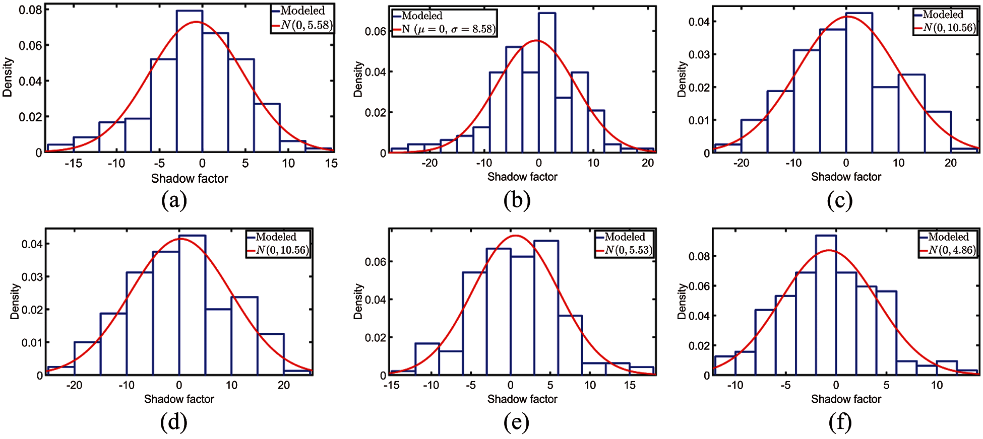
Figure 4: Shadow factor of the different propagation models. (a) CI 3 GHz, (b) CI 28 GHz, (c) CI 28 GHz (TAS); (d) FI 3 GHz, (e) FI 28 GHz, (f) FI 28 GHz (TAS)

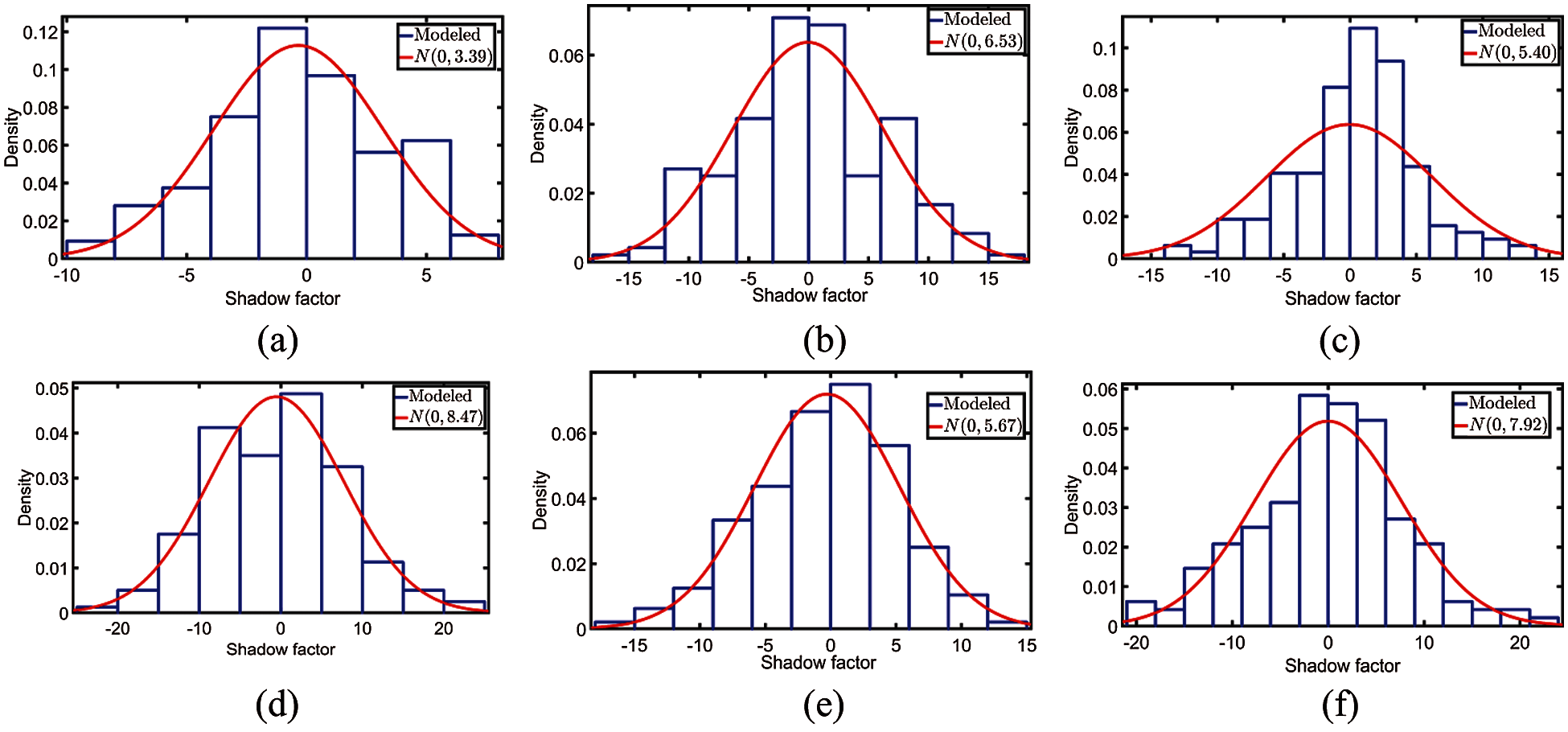
Figure 5: Shadow factor of the different propagation models. (a) CIF 3 GHz, (b) CIF 28 GHz, (c) CIF 28 GHz (TAS); (d) ABG 3 GHz, (e) ABG 28 GHz, (f) ABG, 28 GHz (TAS)

As expected, the histograms generally corresponded to a Gaussian distribution. The experimental mean and standard shadow deviation factors are shown for each Gaussian distribution as a solid red line. The standard deviation values are listed in Tab. 3.

5  Conclusion

This study focused on developing large-scale channel models that characterize wireless path loss in train tunnels. As mentioned earlier, there exists some structural changes in the investigated train tunnel at points 220, 770, 1000, 1260, and 1500 m from the initial measurement position, but no abrupt changes in the received signal strength was noticed at the receiver end (Figs. 3a–3c). Consequently, the effects of such smaller structural shape variations on large-scale wave propagation modelling can be negligible. At every frequency band, the ABG model did not fit well with the measured datasets. While the CI, CIF, and ABG models showed almost similar performance at a frequency of 28 GHz, at 3.7 GHz frequency the FI model suits the measured data more accurately. The FI model showed consistent matching results with the measured datasets at a frequency of 28 GHz for both antenna type horn and the TAS type antenna system. Therefore, the FI model showed better matching performance to the measured datasets than the other models in all measuring scenarios. Given that a lower standard deviation of the shadow factor in the wave propagation model was expected in this case, the FI model yielded shadow factors of 5.49, 5.53, 4.86 at frequencies of 3.7, 28, and 28 GHz (TAS) receivers, respectively. The shadow factors yielded by the FI model are almost the lowest (except for CIF at 3.7 GHz) among all models, as shown in Tab. 3. A minimum shadow factor indicates that the probable error introduced in the model will also be minimal. Additionally, we checked that the point-to-point standard deviation of the received power by the FI model is also minimum among all models, which has not been shown here for brevity. Hence, it can be concluded that the FI model produced more acceptable propagation losses in the tunnel. Based on this investigation, it is assumed that the FI model can predict wave propagation loss in similarly structured train tunnels.

Acknowledgement: The authors would like to thank TA Engineering Inc., South Korea, for assisting with the wave propagation measurement experiments.

Funding Statement: The authors received no specific funding for this study.

Conflicts of Interest: The authors declare that they have no conflicts of interest to report regarding this study.

References

 1.  Z. Hu, W. Ji, H. Zhao, X. Zhai, A. Saleem et al., “Channel measurement for multiple frequency bands in subway tunnel scenario,” International Journal of Antennas and Propagation, vol. 2021, pp. 1–13, 2021. [Google Scholar]

 2.  K. Haneda, L. Tian, H. Asplund, J. Li, Y. Wang et al., “Indoor 5G 3GPP-like channel models for office and shopping mall environments,” in Proc. 2016 IEEE Int. Conf. on Communications Workshops, Kuala Lumpur, Malaysia, pp. 694–699, 2016. [Google Scholar]

 3.  T. S. Rappaport, Y. Xing, G. R. MacCartney, A. F. Molisch, E. Mellios et al., “Overview of millimeter wave communications for fifth-generation (5G) wireless networks—with a focus on propagation models,” IEEE Transactions on Antennas and Propagation, vol. 65, no. 12, pp. 6213–6230, 2017. [Google Scholar]

 4.  A. Hrovat, G. Kandus and T. Javornik, “A survey of radio propagation modeling for tunnels,” IEEE Communications Surveys & Tutorials, vol. 16, no. 2, pp. 658–669, 2014. [Google Scholar]

 5.  A. Seretis, X. Zhang, K. Zeng and C. D. Sarris, “Artificial neural network models for radiowave propagation in tunnels,” IET Microw. Antennas Propag., vol. 14, no. 11, pp. 1198–1208, 2020. [Google Scholar]

 6.  J. Li, Y. Zhao, J. Zhang, R. Jiang, C. Tao et al., “Radio channel measurements and analysis at 2.4/5 GHz in subway tunnels,” China Communications, vol. 12, no. 1, pp. 36–45, 2015. [Google Scholar]

 7.  X. Zhang and C. D. Sarris, “Statistical modeling of electromagnetic wave propagation in tunnels with rough walls using the vector parabolic equation method,” IEEE Transactions on Antennas and Propagation, vol. 67, no. 4, pp. 2645–2654, 2019. [Google Scholar]

 8.  L. Rapaport, G. A. Pinhasi and Y. Pinhasi, “Millimeter wave propagation in long corridors and tunnels—theoretical model and experimental verification,” Electronics, vol. 9, no. 5, pp. 707, 2020. [Google Scholar]

 9.  J. Boksiner, C. Chrysanthos, J. Lee, M. Billah, T. Bocskor et al., “Modeling of radiowave propagation in tunnels,” in Proc. MILCOM 2012–2012 IEEE Military Communications Conf., Orlando, FL, USA, pp. 1–6, 2012. [Google Scholar]

10. M. Liénard and P. Degauque, “Wideband analysis of propagation along radiating cables in tunnels,” Radio Science, vol. 34, no. 1, pp. 113–122, 1999. [Google Scholar]

11. X. Zhang, N. Sood, and C. D. Sarris, “Fast radio-wave propagation modeling in tunnels with a hybrid vector parabolic equation/waveguide mode theory method,” IEEE Transactions on Antennas and Propagation, vol. 66, no. 12, pp. 6540–6551, 2018. [Google Scholar]

12. S. F. Mahmoud, “Wireless transmission in tunnels with non-circular cross section,” IEEE Transactions on Antennas and Propagation, vol. 58, no. 2, pp. 613–616, 2010. [Google Scholar]

13. C. Zhou, “Ray tracing and modal methods for modeling radio propagation in tunnels with rough walls,” IEEE Transactions on Antennas and Propagation, vol. 65, no. 5, pp. 2624–2634, 2017. [Google Scholar]

14. M. M. Rana and A. S. Mohan, “Segmented-locally-one-dimensional-FDTD method for EM propagation inside large complex tunnel environments,” IEEE Transactions on Magnetics, vol. 48, no. 2, pp. 223–226, 2012. [Google Scholar]

15. M. Levy, “Parabolic equation framework,” in Parabolic Equation Methods for Electromagnetic Wave Propagation, Michael Faraday House, Six Hills Way, Stevenage, SG1 2AY, UK: The Institution of Engineering and Technology, pp. 4–19, 2000. [Google Scholar]

16. R. Martelly and R. Janaswamy, “An ADI-PE approach for modeling radio transmission loss in tunnels,” IEEE Transactions on Antennas and Propagation, vol. 57, no. 6, pp. 1759–1770, 2009. [Google Scholar]

17. A. V. Popov and N. Y. Zhu, “Modeling radio wave propagation in tunnels with a vectorial parabolic equation,” IEEE Transactions on Antennas and Propagation, vol. 48, no. 9, pp. 1403–1412, 2000. [Google Scholar]

18. Y. Hwang, Y. P. Zhang and R. G. Kouyoumjian, “Ray-optical prediction of radio-wave propagation characteristics in tunnel environments. 1. Theory,” IEEE Transactions on Antennas and Propagation, vol. 46, no. 9, pp. 1328–1336, 1998. [Google Scholar]

19. Y. P. Zhang and Y. Hwang, “Theory of the radio-wave propagation in railway tunnels,” IEEE Transactions on Vehicular Technology, vol. 47, no. 3, pp. 1027–1036, 1998. [Google Scholar]

20. C. Zhou, R. Jacksha and M. Reyes, “Measurement and modeling of radio propagation from a primary tunnel to cross junctions,” in Proc. 2016 IEEE Radio and Wireless Symposium (RWSAustin, TX, USA, pp. 70–72, 2016. [Google Scholar]

21. H. Qiu, J. M. Garcia-Loygorri, K. Guan, D. He, Z. Xu et al., “Emulation of radio technologies for railways: A tapped-delay-dine channel model for tunnels,” IEEE Access, vol. 9, pp. 1512–1523, 2021. [Google Scholar]

22. F. Hossain, T. K. Geok, T. A. Rahman, M. N. Hindia, K. Dimyati et al., “An efficient 3-D ray tracing method: Prediction of indoor radio propagation at 28 GHz in 5G network,” Electronics, vol. 8, no. 3, pp. 286, 2019. [Google Scholar]

23. S.-H. Chen and S.-K. Jeng, “SBR image approach for radio wave propagation in tunnels with and without traffic,” IEEE Transactions on Vehicular Technology, vol. 45, no. 3, pp. 570–578, 1996. [Google Scholar]

24. C.-H. Teh, B.-K. Chung and E.-H. Lim, “An accurate and efficient 3-d shooting-and- bouncing-polygon ray tracer for radio propagation modeling,” IEEE Transactions on Antennas and Propagation, vol. 66, no. 12, pp. 7244–7254, 2018. [Google Scholar]

25. S. Li, Y. Liu, L. Lin, Z. Sheng, X. Sun et al., “Channel measurements and modeling at 6 GHz in the tunnel environments for 5G wireless systems,” International Journal of Antennas and Propagation, vol. 2017, pp. 1513038, pp. 1–15, 2017. [Google Scholar]

26. I. D. S. Batalha, A. V. R. Lopes, J. P. L. Araujo, B. L. S. Castro, F. J. B. Barros et al., “Indoor corridor and office propagation measurements and channel models at 8, 9, 10 and 11 GHz,” IEEE Access, vol. 7, pp. 55005–55021, 2019. [Google Scholar]

27. N. O. Oyie and T. J. O. Afullo, “Measurements and analysis of large-scale path loss model at 14 and 22 GHz in indoor corridor,” IEEE Access, vol. 6, pp. 17205–17214, 2018. [Google Scholar]

28. Y. Shen, Y. Shao, L. Xi, H. Zhang and J. Zhang, “Millimeter-wave propagation measurement and modeling in indoor corridor and stairwell at 26 and 38 GHz,” IEEE Access, vol. 9, pp. 87792–87805, 2021. [Google Scholar]

29. Keysight Technologies Inc., Technical Overview: Selecting a Signal Generator. [Online]. Available: https://www.keysight.com/kr/ko/assets/7018-03356/technical-overviews/5990-9956.pdf (Accessed on August 23, 2021). [Google Scholar]

30. T. S. Rappaport, “The cellular concept–system design fundamentals,” in Wireless Communications: Principles and Practice, vol. 2. Upper Saddle River, NJ, USA: Prentice-Hall, 1996. [Google Scholar]

31. G. R. MacCartney, J. Zhang, S. Nie and T. S. Rappaport, “Path loss models for 5G millimeter wave propagation channels in urban microcells,” in Proc. 2013 IEEE Global Communications Conf., Atlanta, GA, USA, pp. 3948–3953, 2013. [Google Scholar]

32. J. Meinilä, P. Kyösti, T. Jämsä and L. Hentilä, “WINNER II channel models,” in Radio Technologies and Concepts for IMT-Advanced, 1st ed., 1 Fusionopolis Walk, Solaris South Tower, Singapore, Wiley, pp. 39–92, 2010. [Google Scholar]

33. J. M. Meredith,“Spatial channel model for multiple input multiple output (MIMO) simulations,” Tech-invite, Tech Rep. TR, vol. 25, pp. 1–42, 2012. [Online]. Available: https://www.etsi.org/deliver/etsi_tr/125900_125999/125996/11.00.00_60/tr_125996v110000p.pdf. [Google Scholar]

34. S. Piersanti, L. A. Annoni and D. Cassioli, “Millimeter waves channel measurements and path loss models,” in Proc. 2012 IEEE Int. Conf. on Communications, Ottawa, ON, Canada, pp. 4552–4556, 2012. [Google Scholar]

35. G. R. Maccartney, T. S. Rappaport, S. Sun and S. Deng, “Indoor office wideband millimeter-wave propagation measurements and channel models at 28 and 73 GHz for ultra-dense 5G wireless networks,” IEEE Access, vol. 3, pp. 2388–2424, 2015. [Google Scholar]

36. T. S. Rappaport, G. R. MacCartney, M. K. Samimi and S. Sun, “Wideband millimeter-wave propagation measurements and channel models for future wireless communication system design,” IEEE Transactions on Communications, vol. 63, no. 9, pp. 3029–3056, 2015. [Google Scholar]

37. S. Sun, T. A. Thomas, T. S. Rappaport, H. Nguyen, I. Z. Kovacs et al., “Path loss, shadow fading, and line-of-sight probability models for 5G urban macro-cellular scenarios,” in Proc. 2015 IEEE Globecom Workshops, San Diego, CA, USA, pp. 1–7, 2015. [Google Scholar]

38. A. V. R. Lopes, I. S. Batalha and C. R. Gomes, “Large-scale analysis and modeling for indoor propagation at 10 GHz,” Journal of Microwaves, Optoelectronics and Electromagnetic Applications, vol. 19, no. 2, pp. 276–293, 2020. [Google Scholar]

This work is licensed under a Creative Commons Attribution 4.0 International License, which permits unrestricted use, distribution, and reproduction in any medium, provided the original work is properly cited.