Computers, Materials & Continua DOI:10.32604/cmc.2022.023119
Article

Estimating Weibull Parameters Using Least Squares and Multilayer Perceptron vs. Bayes Estimation

Walid Aydi1,3,* and Fuad S. Alduais2,4

1Department of Computer Science, College of Humanities and Science in Al Aflaj, Prince Sattam Bin Abdulaziz University, Al-Aflaj, Saudi Arabia
2Department of Mathematics, College of Humanities and Science in Al Aflaj, Prince Sattam Bin Abdulaziz University, Al-Aflaj, Saudi Arabia
3Laboratory of Electronics & Information Technologies, Sfax University, Sfax, Tunisia
4Department of Administration, Administrative Science College, Thamar University, Yemen
*Corresponding Author: Walid Aydi. Email: w.aydi@psau.edu.sa
Received: 28 August 2021; Accepted: 25 October 2021

Abstract: The Weibull distribution is regarded as among the finest in the family of failure distributions. One of the most commonly used parameters of the Weibull distribution (WD) is the ordinary least squares (OLS) technique, which is useful in reliability and lifetime modeling. In this study, we propose an approach based on the ordinary least squares and the multilayer perceptron (MLP) neural network called the OLSMLP that is based on the resilience of the OLS method. The MLP solves the problem of heteroscedasticity that distorts the estimation of the parameters of the WD due to the presence of outliers, and eases the difficulty of determining weights in case of the weighted least square (WLS). Another method is proposed by incorporating a weight into the general entropy (GE) loss function to estimate the parameters of the WD to obtain a modified loss function (WGE). Furthermore, a Monte Carlo simulation is performed to examine the performance of the proposed OLSMLP method in comparison with approximate Bayesian estimation (BLWGE) by using a weighted GE loss function. The results of the simulation showed that the two proposed methods produced good estimates even for small sample sizes. In addition, the techniques proposed here are typically the preferred options when estimating parameters compared with other available methods, in terms of the mean squared error and requirements related to time.

Keywords: Weibull distribution; maximum likelihood; ordinary least squares; MLP neural network; weighted general entropy loss function

1  Introduction

The parameters of the Weibull distribution are widely used in reliability studies and many engineering applications, such as the lifetime analysis of material strength [1], estimation of rainfall [2], hydrology [3], predictions of material and structural failure [4], renewable and alternative energies [5–8], power electronic systems [9], and many other fields [10–12].

The form of the probability density function (PDF) of two parameters of WD is given by:

f(x;ϑ,λ)=λϑ(xϑ)(λ−1)exp⁡[−(xϑ)λ],x>0ϑ,λ>0(1)

The cumulative distribution function (CDF) and the survival function S of the WD can be expressed as

F(x;ϑ,λ)=1−exp⁡[−(xϑ)λ],x>0ϑ,λ>0(2)

S(t;ϑ,λ)=exp⁡[−(tϑ)λ],t>0ϑ,λ>0(3)

where the parameters ϑ and λ represent the scale and the shape of the distribution, respectively.

Several approaches to estimating the parameters of the WD have been proposed [13]. They can generally be classified as manual or numerical [14].

Manual approaches include the ordinary least squares [15,16], unbiased good linear estimators [17], and weighted least squares [18]. Computational methods include maximum likelihood estimation [19], the moments estimation method [20], Bayesian approach [21], and least-squares estimation with particle swarm optimization [22].

In addition to computational methods, many studies in the literature have attempted to use the neural network (NN) to anticipate the parameters of the WD in many areas, such as the method developed by Jesus that applies the Weibull and ANN analysis to anticipate the shelf life and acidity of vacuum-packed fresh cheese [23]. In survival analysis, Achraf constructed a deep neural network model called DeepWeiSurv. It was assumed that the distribution of survival times follows a finite mixture of a two-parameter WD [24]. In another work in the field of electric power generation, an artificial NN (ANN) and q-Weibull were applied to the survival function of brushes in hydroelectric generators [25].

Recently, a few methods have been attempted to combine the robustness of the ANN and some of the above statistical methods. Maria modeled the distribution of tree diameters using the OLS and the ANN [26]. In the same way and based on the ability of the OLS, in its simplest form, which assumes a linear relationship between the predictor and the unreliability function on one hand and the robustness and rapidness of the single-hidden-layer networks to handle the linear functions compared with multiple-hidden-layer [27] on the other hand, we will propose to combine OLS and a neural network to predict the two-parameter WD.

In the proposed method, we solve the problem whereby the reliability of the OLS method is compromised by outliers through the introduction of a pre-trained neural network after the linearization of the CDF. The remaining sections of this paper are organized as follows: Section 2 provides a review of different numerical and graphical methods for estimating the parameters of the WD, such as the MLE, OLS, WLS, and BLGE. In Section 3 we present the proposed methods. To evaluate their appropriateness in comparison with competing methods, the relevant performance metrics are covered in Section 4. The results are discussed in Section 5. Finally, the conclusions of this study are provided in Section 6.

2  Review of Numerical and Graphical Methods for Estimating Parameters of WD

The most commonly used approaches to estimate the parameters λ and ϑ of the WD are described below.

2.1 Maximum Likelihood Estimator (MLE)

Let the set (x1,x2,x3,…xn) of n random lifetimes from the WD be defined by Eq. (1). Then, the likelihood function Lf and its corresponding logarithm ℓ for the given sample observations are shown in Eqs. (4) and (5), respectively [28]:

Lf(x_;ϑ,λ)=∏i=1n⁡λϑ(xiϑ)λ−1exp⁡[−(xϑ)λ],(4)

ℓ=nlnλ−nλlnϑ+(λ−1)∑i=1n⁡lnxi−∑i=1n⁡(xiϑ)λ(5)

The partial derivatives of the equation for ℓ with respect to the variables ϑ and λ are given by:

∂ℓ∂ϑ=−n(λϑ^)+λϑ^∑i=1n⁡(xiϑ^)=0,(6)

∂ℓ∂λ=nλ^+∑i=1n⁡(xiϑ)−∑i=1n⁡(xiϑ)λln(xiϑ)=0(7)

The MLE estimator ϑ^MLE of ϑ is:

ϑ^MLE=[1n∑i=1n⁡(xi)λ^]1λ^(8)

The parameter λ can be obtained by using any numerical method, such as the Newton–Raphson.

2.2 Ordinary Least Squares Method (OLS)

To estimate the parameters of the WD, the OLS method is extensively used in mathematics and engineering problems [16]. We can obtain a linear relationship between parameters by taking the logarithm of Eq. (2) as follows:

ln[−ln(1−F(x;ϑ,λ)]=−λlnϑ+λlnx(9)

Let Yi=ln[−ln(1−F(xi;ϑ,λ))],Xi=lnx(i),α0=−λlnϑ,andβ=λ. Then, Eq. (9) can be written as Yi=α0+βXi+ϵi

Let X(1),X(2),X(3),…X(n) be order statistics of X1,X2,X3,…Xn, and let x(1)<  x(2) <x(3)<…<x(n) be the ordered observations in a random sample of size n. To estimate the values of the cumulative distribution function F(x(i)ϑ,λ), we use the mean rank method as follows:

F^(xi)=(i−0.3)/(n+0.4),i=1,2,3,…,n(10)

The estimates α^0 and β^ of the regression parameters α0 and β minimize the function

Q(a,b)=∑i=1n⁡(Yi−α0−βlnx(i))2(11)

Therefore, the estimates α^0 and β^ of the parameters α0 and β are given by

β^OLS=n∑i=1n⁡lnx(i)ln[−ln(1−F^(xi)))]−∑i=1n⁡lnxi∑i=1n⁡ln[−ln(1−F^(xi)))]n∑i=1n⁡ln2(xi)−(∑i=1n⁡lnx(i))2(12)

α^0OLS=1n∑i=1nln[−ln(1−F^(xi)))]−β^OLS1n∑i=1nlnx(i)(13)

The estimates λ^OLS and ϑ^OLS of the parameters λ and ϑ are given by

λ^OLS=n∑i=1n⁡lnxiln[−ln(1−F^i)]−∑i=1n⁡lnxi∑i=1n⁡ln[−ln(1−F^i))]n∑i=1n⁡ln2(xi)−(∑i=1n⁡lnx(i))2(14)

ϑ^OLS=exp[−∑i=1n⁡ln[−ln(1−F^i))]−β^OLS∑i=1n⁡lnx(i)nβ^OLS](15)

2.3 Weighted Least Squares Method (WLS)

In the WLS estimate, the parameters λ  and ϑ are the values of the parameters that minimize the function:

Q∗W(λ,ϑ)=∑i=1n⁡Wi(ln[−ln(1−F^(xi))]+lnϑ−λlnx(i))2(16)

The biggest challenge in the application of the WLS is in finding the weights {\cal W}i in Eq. (15). We use the delta method [29] to find them:

Var(ln[−ln(1−F^(xi))])∝1[(1−F^(xi))ln(1−F^(xi))]2(17)

Hence, the weights can be written as follows:

Wi=[(1−F^(xi))ln(1−F^(xi))]2∑i=1n⁡[(1−F^(xi))ln(1−F^(xi))]2,i=1,2,3,…,n.(18)

Minimizing Q∗W(λ,ϑ) we obtain the WLS estimates of λ and ϑ as

λ^WOLS=∑i=1n⁡WiDiAi−(∑i=1n⁡WiDi)(∑i=1n⁡WiAi)∑i=1n⁡WiDi2−(∑i=1n⁡WiDi)2(19)

ϑ^WOLS=exp⁡[ψ^Wλ^WOLS],(20)

where

 ψ^{\cal W}=λ^WOLS∑i=1n⁡{\cal W}i{\cal D}i−∑i=1n⁡{\cal W}i{\cal A}i, with {\cal D}i=lnx(i) and {\cal A}i=ln[−ln(1−F^(xi))]

2.4 Approximate Bayes Estimator

In this section, the approximate Bayesian estimator under a GE loss function of the parameters λ and ϑ of the WD is discussed. We assume a non-informative (vague) prior according to [30] as

π(λ,φ)∝1λϑ(21)

The parameters λ and φ are estimated using Lindley's approximation technique. The posterior expectation E is given by Eq. (22) [31]:

E[u(ϕ)|x]=∫Ω⁡u(ϕ)π(ϕ)L(ϕ|x)dϕ∫Ω⁡π(ϕ)L(ϕ|x)dϕ(22)

Moreover, it can be asymptotically estimated by:

E[u(ϕ)|x]=u+12∑i⁡∑j⁡(uij+2uiρj)σij+12∑i⁡∑j⁡∑k⁡∑l⁡Lijkσijσklui(23)

where i,j,k,l=1,2,…m,ϕ=(ϕ1,ϕ1,…ϕm), π(ϕ) represents the prior distribution of ϕ,u=u(ϕ), L=L(ϕ) is the likelihood function, ρ≡ρ(ϕ)=ln⁡(π(ϕ)),ρi=∂ρ∂ϕi, ui=∂u∂ϕi, uij=∂2u∂ϕi∂ϕj,Lijk=∂3L∂ϕi∂ϕj∂ϕk, and σij=element(i,j) of the covariance matrix of the parameter estimators.

For the two-parameter case ϕ=(λ,φ), Eq. (22) reduces to:

E[(ϕ|x)]=u+12[u11σ11+u22σ22]+u1ρ1σ11+u2ρ2σ22+12[L30u1σ112+L03u2σ222](24)

The functions in Eq. (24) are computed using MLEs with respect to λ and φ.

To apply the Lindley model of Eq. (24) to estimate the parameters of the WD, the following are obtained from Eq. (23):

The elements σij of the covariance matrix are expressed by

2.4.1 Estimates Based on General Entropy Loss Function

The general entropy loss function L for ϕ, shown in Eq. (24), is expressed by the following form [32]:

L(ϕ^,ϕ)∝(ϕ^ϕ)q−qln(ϕ^ϕ)−1,q≠0,(25)

where ϕ^  is an estimate of ϕ. The Bayes estimator of ϕ, denoted by ϕ^GE, is the value ϕ^ that minimizes Eq. (26):

ϕ^GE=[Eϑ(ϕ−q)]−1q(26)

The BLGE of λ^BLGE for λ from Eq. (24) is found by the following expressions:

In the same way, the BLGE of ϑ^BLGE for ϑ is found by the following expressions:

3  Proposed Methods

In the following sections, we describe the proposed BLWGE and OLSMLP methods.

3.1 Weighted General Entropy Loss Function

The WGE loss function was proposed as dependent on the weighted loss GE function as follows:

Lw(ϕ^,ϕ)∝w(ϕ)[(ϕ^ϕ)q−qln(ϕ^ϕ)−1],q≠0(27)

where ϕ represents the estimated parameters that minimize the expectation of the loss function (Eq. (27)), and w(ϕ) represents the proposed weighted function as expressed by Eq. (28):

w(ϕ)=1ϕz(28)

Based on the posterior distribution of the parameter ϕ, and by using the WGE function given in Eq. (28), we obtain the estimated BLWGE of the parameter ϑ as follows:

Thus, we can find that

Consequently, the BLWGE of parameter ϕ, obtained by using the WGE loss function, is ϕ^BLWGE as presented in Eq. (29):

ϕ^WGE=E(ϕ−(z+q)|x_)E(ϕ−z)|x_)where,z+q≠0(29)

provided that Eϕ(ϕ−z) and Eϕ(ϕ−(z+q)) exist and are finite, where Eϕ represents the expected value.

We note that the GE is a special case of the WGE when z=0 in Eq. (29).

3.1.1 Estimates of Parameters of WD Based on Weighted General Entropy Loss Function

Based on the WGE and by using Eq. (29), the approximate Bayes estimator λ^BLWGE for λ is shown as:

λ^BLWGE=[E(λ−(z+q)|x_)E(λ−z)|x_)]−1q=[I1I2]−1q(30)

where

I1=u∗+12[u11∗σ11+u22∗σ22]+u1∗ρ1σ11+u2∗ρ2σ22+12[L30u1∗σ112+L03u2∗σ222](31)

and

I2=u∗∗+12[u11∗∗σ11+u22∗∗σ22]+u1∗∗ρ1σ11+u2∗∗ρ2σ22+12[L30u1∗∗σ112+L03u2∗∗σ222](32)

Thus, the BLWGE λ^BLWGE for the shape parameter λ is

λ^WGE[I1I2]−1q=[u∗+12[u11∗σ11+u22∗σ22]+u1∗ρ1σ11+u2∗ρ2σ22+12[L30u1∗σ112+L03u2∗σ222]u∗∗+12[u11∗∗σ11+u22∗∗σ22]+u1∗∗ρ1σ11+u2∗∗ρ2σ22+12[L30u1∗∗σ112+L03u2∗∗σ222]]−1q(33)

Similarly, the BLWGE ϑ^BLWGE for ϑ, is given by Eq. (34):

ϑ^WGE=[E(ϑ−(z+q)|x_)E(ϑ−z)|x_)]−1q=[I3I4]−1q(34)

where

I3=ν+12[ν11σ11+ν22σ22]+ν1ρ1σ11+ν2ρ2σ22+12[L30ν1σ112+L03ν2σ222](35)

and

I4=ν∗+12[ν11∗σ11+ν22∗σ22]+ν1∗ρ1σ11+ν2∗ρ2σ11+12[L30ν1∗σ112+L03ν2∗σ222](36)

Thus, the weighted Bayes estimator for the shape parameter ϑ is

ϑ^BLWGE[I3I4]−1q=[ν+12[ν11σ11+ν22σ22]+ν1ρ1σ11+ν2ρ2σ22+12[L30ν1σ112+L03ν2σ222]ν∗+12[ν11∗σ11+ν22∗σ22]+ν1∗ρ1σ11+ν2∗ρ2σ11+12[L30ν1∗σ112+L03ν2∗σ222]]−1q(37)

3.2 Ordinary Least Squares and the Multilayer Perceptron Neural Network (OLSMLP)

As previous studies have shown [14,33], manual calculations yield the smallest standard deviation (STD) in the parameter λ, and are consequently more accurate than computational methods. Moreover, methods of manual estimation are more accurate for small sample sizes [14]. However, these computational methods, especially the OLS, are sensitive to outliers and specific residual behavior [34]. To solve these problems, many studies have proposed different methods, such as the iterative weighting method based on the modified OLS [34], the WLS, and many other methods based on the WLS [35]. A major challenge in these methods is determining the weights.

3.2.1 Proposed Method to Estimate Parameters of WD

We now describe the proposed method, which is divided into two main parts: the linearization of the CDF, and the application of a feedforward network with backpropagation to estimate the values of λ and ϑ of the WD.

The OLS method takes the CDF defined in Eq. (2) and linearizes it as described in Eq. (10). It then determines the coefficients α0 and β via linear regression by using the slope and the intercept. The principle of the method used by the OLS to compute α0 and β can be violated even with a few outliers.

Therefore, instead of using the slope and the intercept, we propose applying Algorithm 1 as described below.

•   Application of Proposed Model to Estimate Parameters of WD

The steps used to evaluate the parameters of the WD from the input csv file are described by Algorithm 1.

•   Data Normalization

Normalization is an essential preprocessing tool for a neural network [36,37]. Before training a neural network model, the input data are scaled using the RobustScaler norm in a preliminary phase, where each sample with at least one non-zero component is rescaled using the median and quartile range as described by Eq. (38). The RobustScaler norm is used to remove the influence of outliers. Following this, the MinMaxScaler, defined by Eq. (39), is applied to the output of the RobustScaler. The MinMaxScaler scales all the data features to the range [0, 1]:

Xism=Xi−Q1(X)Q3(X)−Q1(X)(38)

where X is a feature vector, Xi is an element of feature X, Xism is the rescaled element obtained by using MinMaxScaler, and Xisr is the rescaled element obtained by using RobustScaler.

Xisr=Xisr−min(Xsr)max(Xsr)−min(Xsr)(39)

•   Structure of the Proposed Neural Network

To estimate the parameters of the WD, we propose using a multilayer perceptron (MLP), which is a feedforward network with backpropagation [38]. According to the structure of the MLP, the proposed network, as shown in Fig. 1, consists of an input layer (with n neurons), a hidden layer (with k neurons), and an output layer (with m neurons that yield the Weibull parameters as the output of the network).

Figure 1: Topology of the proposed MLP

Various criteria have been proposed in the literature to fix the number of hidden neurons [39]. In our architecture, we use the rule whereby “the number of hidden neurons k should be 2/3 times the size of the input layer, plus the size of the output layer” [38–40].

The hyperbolic tangent activation function (tanh) is proposed here in the input layer, and the sigmoid function in the output layer. They are used frequently in feedforward nets, and are suitable for shallow networks as well as applications of prediction and mapping [38,41].

The objective of our neural network is a model that performs well on the data used in both the training and the test datasets. For this reason, we add a well-known regularization layer as described in the next section.

•   Regularization

Regularization is a technique that can prevent overfitting [37,38]. A number of regularization techniques have been develop in the literature, such as L1 and L2 regularizations, bagging, and dropout. In the proposed structure, we use dropout, a well-known technique that randomly “drops out” or omits hidden neurons of the neural network to make them unavailable during part of the training [38,42]. This reduces the co-adaption between neurons, which results in less overfitting [38].

•   Optimization Algorithm

The optimization of deep networks is an active area of research [43]. The most popular gradient-based optimization algorithms are Adagrad, Momentum, RMSProp, Adam, AdaDelta, AdaMax, Nadam, and AMSGrad [38,43,44]. We chose Nadam due to its superiority in supervised machine learning over the other techniques, especially for a deep network [43]. Moreover, it combines the strengths of the Nesterov acceleration gradient (NAG) and the adaptive estimation (Adam) algorithms as described in [44]:

wt+1=wt−αnadvt^+ε(β1m^t+1−β11−β1t∗∂L∂wt)(40)

where

t: time step

αnad : learning rate

vt: the exponential average square of gradients

mt: momentum vector

wt: the weight that we want to update

ε: smoothing term

∂L∂wt: gradient of L; the loss function to minimize.

β1,β2: momentum decay and scaling decay, respectively

4  Performance Metrics

To evaluate the proposed methods with respect to other methods, we used two statistical tools, the mean squared error (MSE) and the mean absolute percentage error (MAPE) [5], in addition to the computation time.

5  Results and Discussion

5.1 Dataset Description

We generated 250,000 random data points from the WD for different parameters and different values of ϑ ranging from 1 to 299, and those of λ ranging from 0.5 to 100. For each shape/scale pair, we generated 10,000 samples of different sizes n=10,20,30,40,and50.

We used the same dataset for the neural network in the training phase, but applied one sample to each shape/scale pair. This was unlike in the other methods (MLE, OLS, WLS, BLGE, and BLWGE), which used 10,000 samples to estimate the parameters of the WD. This dataset was divided into two subsets. The first subset was used to fit the model, and is referred to as the training dataset; it was characterized by known inputs and outputs. The second subset is referred to as the test dataset, and was used to evaluate the fitted machine learning model and make predictions on the new subset, for which we did not have the expected output. We chose the train–test procedure for our experiments because we guessed that we had a sufficiently large dataset available.

5.2 Experimental Setting

5.2.1 Parameter Selection for OLSMLP

In all experiments, we trained the model with Google Collaboratory (GPU) for 25 epochs. We used the Nadam optimizer with learning rate of αnad=0.001; terms representing the momentum decay, scaling decay, and smoothing were kept at their default values: β1=0.9, β2=0.999, and ε=10−7. A dropout with a ratio of 0.6 was applied to the hidden layer. As described in Section 3, the hidden and output layers used the tanh and sigmoid activation functions, respectively. The error function or loss function was the mean squared error, and was used to estimate the loss of the model.

5.2.2 Parameter Selection of BLGE and BLWGE

In all experiments, the parameters of the BLWGE and BLGE were empirically determined. The values of the weights q and z of the BLWGE were −3 and 6, respectively. For the BLGE, the parameter q=1.5.

5.3 Estimating Parameters of Weibull Distribution

5.3.1 Effect of Sample Size on Estimation of WD Parameters Using Prevalent Methods

Fig. 2 shows the evolution of the average MSE as a function of the sample size n. The MSE decreased quasi-linearly from n=10 to n=40 for all methods. Fig. 2 shows that the BLWGE, WLS, BLGE, and MLE had the lower MSE values for the different sample sizes compared with the OLS. We can deduce also that the WLS, GE, and MLE gave similar results with a slightly better start for the MLE at n=10.

Figure 2: The evolution of the MSE using the parameters ϑ=2.5 and λ = 1.685 as a function of n=[10−40] for the MLE, OLS, WLS, BLGE, and BLGWGE

5.3.2 Effect of Sample Size on Estimation of WD Parameters Using Proposed Method

To illustrate how the sample size affects the calculation of the MSE, Fig. 3 shows the evolution of the latter as a function of the sample size n from 10 to 50.

Figure 3: The evolution of the MSE using the parameters ϑ=0.75 and λ = 1.75 as a function of n=[10−50]

From Fig. 3, we can deduce that as the sample size increased, the estimate of the MSE by the proposed method decreased and fluctuated. This fluctuation was due to the random nature of the information used and the limited number of samples (one sample) for each pair of shapes/scales.

Tabs. 1 and 2 show the results of the simulation of the proposed method and the other methods considered above. The results show the following:

1. The MLE and WLS behaved similarly as shown in Tab. 1: Their MSE values decreased gradually when their shape values increased at a fixed scale. Conversely, when the scale value increased with a fixed shape, the MSE increased.

2. The behavior of the OLS and GE was the opposite of that of the MLE and WLS. As depicted in Tab. 1, the MSE increased when the shape increased (at a fixed scale), and decreases when the scale increased (with a fixed shape).

3. The BLWGE and the OLSMLP behaved similarly in terms of scale estimation, as shown in Tab. 1.

4. All methods had the same global variation function, as shown in Fig. 4 and Tab. 2.

5. The MLE was slightly superior globally in terms of scale estimation to the other methods, but had the worst estimation of shape, as shown in Tab. 2.

6. The proposed MLP neural network acceptably estimated the scale, better than some methods. By contrast, it outperformed all other methods in terms of shape estimations most of the time.

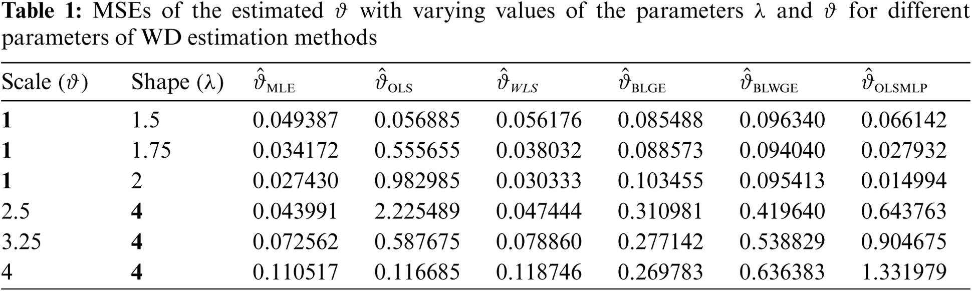
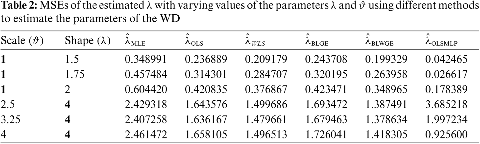
Figure 4: MSEs of λ^ with varying values of the parameters ϑ=[1112.53.254] and λ=[1.51.752444] for the MLE, OLS, BLGE, WLS, and the proposed methods

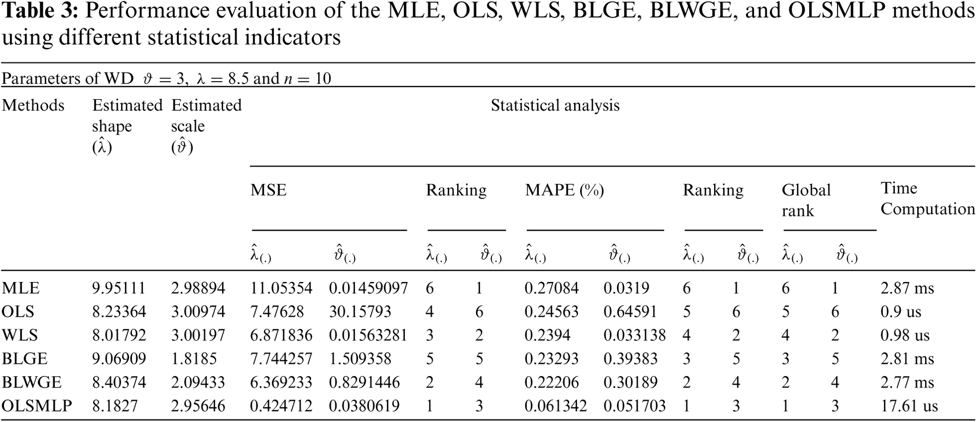
From Tab. 3, we see that both statistical indicators, MSE and MAPE, yielded different values. The global rank was calculated to evaluate the best method. The results in the table indicate that the proposed method offered the best compromise between shape and scale estimation, as indicated by the global rank. Moreover, it retained the speed of the OLS and enhanced the accuracy of estimation of the parameters of the WD compared with the MLE, BLGE, and BLWGE.

6  Conclusion

This study proposed a method to estimate the parameters of the WD. This method is based on the OLS graphical method and the MLP neural network. The MLP solves the problems caused by the presence of outliers and eases the difficulty of determining the weights in the WLS method. It yielded acceptable results in simulations, especially in terms of shape estimation. It is also faster than the MLE, BLGE, and BLWGE.

We also proposed a second method (BLWGE), in which we introduced weight to the GE loss function. The results of simulations showed that BLWGE yields good results, especially in terms of shape estimation, compared with the other methods.

Acknowledgement: This project was supported by the Deanship of Scientific Research at Prince Sattam bin Abdulaziz University under Research Project No. 2020/01/16725.

Funding Statement: The authors are grateful to the Deanship of Scientific Research at Prince Sattam bin Abdulaziz University Supporting Project Number (2020/01/16725), Prince Sattam bin Abdulaziz University, Saudi Arabia.

Conflicts of Interest: The authors declare that they have no conflicts of interest to report regarding this study.

References

 1.  M. R. Piña-Monarrez, “Weibull stress distribution for static mechanical stress and its stress/strength analysis,” Quality and Reliability Engineering International, vol. 34, no. 2, pp. 229–244, 2018. [Google Scholar]

 2.  A. Alonge and T. Afullo, “Rainfall drop-size estimators for Weibull probability distribution using method of moments technique,” SAIEE Africa Research Journal, vol. 103, no. 2, pp. 83–93, 2012. [Google Scholar]

 3.  F. Ashkar, I. Ba and B. B. Dieng, “Hydrological frequency analysis: Some results on discriminating between the Gumbel or Weibull probability distributions and other competing models,” in World Environmental and Water Resources Congress: Watershed Management, Irrigation and Drainage, and Water Resources Planning and Management, Reston, VA: American Society of Civil Engineers, pp. 374–387, 2019. [Google Scholar]

 4.  C. W. Yang and S. J. Jiang, “Weibull statistical analysis of strength fluctuation for failure prediction and structural durability of friction stir welded Al–Cu dissimilar joints correlated to metallurgical bonded characteristics,” Materials, vol. 12, no. 2, pp. 205, 2019. [Google Scholar]

 5.  P. K. Chaurasiya, S. Ahmed and V. Warudkar, “Study of different parameters estimation methods of Weibull distribution to determine wind power density using ground based Doppler SODAR instrument,” Alexandria Engineering Journal, vol. 57, no. 4, pp. 2299–2311, 2018. [Google Scholar]

 6.  H. H. Surendra, D. Seshachalam and K. R. Sudhindra, “Reliability analysis of solar energy resources using Weibull distribution for a standalone system in Indian context,” International Journal of Scientific Research in Mathematical and Statistical Sciences, vol. 7, pp. 64–68, 2020. [Google Scholar]

 7.  M. Bassyouni, S. A. Gutub, U. Javaid, M. Awais, S. Rehman et al., “Assessment and analysis of wind power resource using Weibull parameters,” Energy Exploration & Exploitation, vol. 33, no. 1, pp. 105–122, 2015. [Google Scholar]

 8.  M. Sumair, T. Aized, S. A. R. Gardezi, S. U. Ur Rehman and S. M. S. Rehman, “Wind potential estimation and proposed energy production in Southern Punjab using Weibull probability density function and surface measured data,” Energy Exploration & Exploitation, vol. 39, pp. 2150–2168, 2020. [Google Scholar]

 9.  B. Rackauskas, M. J. Uren, T. Kachi and M. Kuball, “Reliability and lifetime estimations of GaN-on-GaN vertical pn diodes,” Microelectronics Reliability, vol. 95, pp. 48–51, 2019. [Google Scholar]

10. B. B. Sagar, R. K. Saket and C. G. Singh, “Exponentiated Weibull distribution approach-based inflection S-shaped software reliability growth model,” Ain Shams Engineering Journal, vol. 7, no. 3, pp. 973–991, 2016. [Google Scholar]

11. E. J. Tuegel, R. P. Bell, A. P. Berens, T. Brussat, J. W. Cardinal et al., “Aircraft structural reliability and risk analysis handbook.” Air Force Research Lab. Wright-Patterson Air Force Base, 2013. [Google Scholar]

12. Q. Fu, H. Wang and X. Yan, “Evaluation of the aeroengine performance reliability based on generative adversarial networks and Weibull distribution,” Proceedings of the Institution of Mechanical Engineers, Part G: Journal of Aerospace Engineering, vol. 233, no. 15, pp. 5717–5728, 2019. [Google Scholar]

13. M. Sumair, T. Aized, S. A. R. Gardezi and M. Waqas Aslam, “Efficiency comparison of historical and newly developed Weibull parameters estimation methods,” Energy Exploration & Exploitation, vol. 39, pp. 1–22, 2020. [Google Scholar]

14. K. C. Datsiou and M. Overend, “Weibull parameter estimation and goodness-of-fit for glass strength data,” Structural Safety, vol. 73, pp. 29–41, 2018. [Google Scholar]

15. J. Maroco, “Consistency and efficiency of ordinary least squares, maximum likelihood, and three type II linear regression models: A monte carlo simulation study,” Methodology: European Journal of Research Methods for the Behavioral and Social Sciences, vol. 3, no. 2, pp. 81, 2007. [Google Scholar]

16. J. Cohen, P. Cohen, S. G. West and L. S. Aiken, in Applied Multiple Regression/Correlation Analysis for the Behavioral Sciences, Mahwah, N.J: Lawrence Erlbaum Associates, Routledge, New York, 2002. [Google Scholar]

17. M. Engelhardt and L. J. Bain, “Simplified statistical procedures for the Weibull or extreme-value distribution,” Technometrics, vol. 19, no. 3, pp. 323–331, 1977. [Google Scholar]

18. K. Jabłońska, “Dealing with heteroskedasticity giving the example of modelling quality of life of older people,” Statistics in Transition, New Series, vol. 19, no. 3, pp. 433–452, 2018. [Google Scholar]

19. H. Saleh, A. E. A. Aly and S. Abdel-Hady, “Assessment of different methods used to estimate Weibull distribution parameters for wind speed in Zafarana wind farm, Suez Gulf, Egypt,” Energy, vol. 44, no. 1, pp. 710–719, 2012. [Google Scholar]

20. R. B. Abernethy, in the New Weibull Handbook: Reliability and Statistical Analysis for Predicting Life, Safety, Supportability, Risk, Cost and Warranty Claims, 5th edition, Hickory: Barringer & Associates, 2006. [Google Scholar]

21. K. Ullah, M. Aslam and T. N. Sindhu, “Bayesian analysis of the Weibull paired comparison model using informative prior,” Alexandria Engineering Journal, vol. 59, no. 4, pp. 2371–2378, 2020. [Google Scholar]

22. N. Qiu, Q. Liu and Z. Zeng, “Particle swarm optimization and least squares method for geophysical parameter inversion from magnetic anomalies data,” in 2010 IEEE Int. Conf. on Intelligent Computing and Intelligent Systems, Xiamen, China, pp. 879–881, 2010. [Google Scholar]

23. J. A. Sánchez-González and J. F. Oblitas-Cruz, “Application of Weibull analysis and artificial neural networks to predict the useful life of the vacuum-packed soft cheese,” Revista Facultad de Ingeniería Universidad de Antioquia, vol. 82, pp. 53–59, 2017. [Google Scholar]

24. A. Bennis, S. Mouysset and M. Serrurier, “Estimation of conditional mixture Weibull distribution with right censored data using neural network for time-to-event analysis,” in 2020 Pacific-Asia Conf. on Knowledge Discovery and Data Mining, Singapore, pp. 687–698, 2020. [Google Scholar]

25. E. M. De Assis, C. L. S. Figueirôa Filho, G. A. D. C. Lima, L. A. N. Costa and G. M. D. O. Salles, “Machine learning and q-Weibull applied to reliability analysis in hydropower sector,” IEEE Access, vol. 8, pp. 203331–203346, 2020. [Google Scholar]

26. M. J. Diamantopoulou, R. Özçelik, F. Crecente-Campo and Ü. Eler, “Estimation of Weibull function parameters for modelling tree diameter distribution using least squares and artificial neural networks methods,” Biosystems Engineering, vol. 133, pp. 33–45, 2015. [Google Scholar]

27. T. Nakama, “Comparisons of single-and multiple-hidden-layer neural networks,” in 2011 Conf. Advances in Neural Networks, Guilin, China, vol. 6675, pp. 270–279, 2011. [Google Scholar]

28. S. Abdulah, H. Ltaief, Y. Sun, M. G. Genton and D. E. Keyes, “Parallel approximation of the maximum likelihood estimation for the prediction of large-scale geostatistics simulations,” in 2018 IEEE Conf. on Cluster Computing (CLUSTERBelfast, UK, pp. 98–108, 2018. [Google Scholar]

29. W. L. Hung and Y. C. Liu, “Estimation of Weibull parameters using a fuzzy least-squares method,” International Journal of Uncertainty, Fuzziness and Knowledge-Based Systems, vol. 12, no. 5, pp. 701–711, 2004. [Google Scholar]

30. S. K. Sinha and J. A. Sloan, “Bayes estimation of the parameters and reliability function of the 3-parameter Weibull distribution,” IEEE Transactions on Reliability, vol. 37, pp. 364–369, 1988. [Google Scholar]

31. L. M. Lye, K. P. Hapuarachchi and S. Ryan, “Bayes estimation of the extreme-value reliability function,” IEEE Transactions on Reliability, vol. 42, no. 4, pp. 641–644, 1993. [Google Scholar]

32. R. Calabria and G. Pulcini, “Point estimation under asymmetric loss functions for left-truncated exponential samples,” Communications in Statistics-Theory and Methods, vol. 25, no. 3, pp. 585–600, 1996. [Google Scholar]

33. F. N. Nwobi and C. A. Ugomma, “A comparison of methods for the estimation of Weibull distribution parameters,” Metodoloski Zvezki, vol. 11, no. 1, pp. 65, 2014. [Google Scholar]

34. M. Bashiri and A. Moslemi, “The analysis of residuals variation and outliers to obtain robust response surface,” Journal of Industrial Engineering International, vol. 9, no. 1, pp. 1–10, 2013. [Google Scholar]

35. L. F. Zhang, M. Xie and L. C. Tang, “On weighted least squares estimation for the parameters of Weibull distribution,” in Recent Advances in Reliability and Quality in Design, London, UK: Springer, pp. 57–84, 2008. [Google Scholar]

36. E. Hoffer, R. Banner, I. Golan and D. Soudry, “Norm matters: Efficient and accurate normalization schemes in deep networks,” in 2018 32nd Conf. on Neural Information Processing Systems, Montréal, Canada, 2018. [Google Scholar]

37. G. Abosamara and H. Oqaibi, “An optimized deep residual network with a depth concatenated block for handwritten characters classification,” Computers Materials & Continua, vol. 68, no. 1, pp. 1–28, 2021. [Google Scholar]

38. J. Heaton, in Artificial Intelligence for Humans, 3rd edition, vol. 1, St. Louis: Charleston Createspace, 2015. [Google Scholar]

39. K. G. Sheela and S. N. Deepa, “Review on methods to fix number of hidden neurons in neural networks,” Mathematical Problems in Engineering, vol. 2013, pp. 1–11, 2013. [Google Scholar]

40. J. Heaton, “The number of hidden layers,” 2021, [online]. Available: https://www.heatonresearch.com/2017/06/01/hidden-layers.html [Accessed 19 April 2021]. [Google Scholar]

41. T. Szandała, “Review and comparison of commonly used activation functions for deep neural networks,” in Bio-inspired Neurocomputing, Singapore: Springer, pp. 203–224, 2021. [Google Scholar]

42. N. Srivastava, G. Hinton, A. Krizhevsky, L. Sutskever and R. Salakhutdinov, “Dropout: A simple way to prevent neural networks from overfitting,” Journal of Machine Learning Research, vol. 15, no. 1, pp. 1929–1958, 2014. [Google Scholar]

43. D. Soydaner, “A comparison of optimization algorithms for deep learning,” International Journal of Pattern Recognition and Artificial Intelligence, vol. 34, no. 13, pp. 2052013, 2020. [Google Scholar]

44. E. M. Dogo, O. J. Afolabi, N. I. Nwulu, B. Twala and C. O. Aigbavboa, “A comparative analysis of gradient descent-based optimization algorithms on convolutional neural networks,” in 2018 Conf. on Computational Techniques, Electronics and Mechanical Systems, Belgaum, India, pp. 92–99, 2018. [Google Scholar]

This work is licensed under a Creative Commons Attribution 4.0 International License, which permits unrestricted use, distribution, and reproduction in any medium, provided the original work is properly cited.