Computers, Materials & Continua DOI:10.32604/cmc.2022.023126
Article

Gaining-Sharing Knowledge Based Algorithm for Solving Stochastic Programming Problems

Prachi Agrawal1, Khalid Alnowibet2 and Ali Wagdy Mohamed3,4,*

1Yogananda School of Artificial Intelligence, Computers & Data Science, Shoolini University, Solan, 173229, India
2Statistics and Operations Research Department, College of Science, King Saud University, Riyadh, 11451, Kingdom of Saudi Arabia
3Operations Research Department, Faculty of Graduate Studies for Statistical Research, Cairo University, Giza, 12613, Egypt
4Department of Mathematics and Actuarial Science, School of Science and Engineering, The American University in Cairo, Egypt
*Corresponding Author: Ali Wagdy Mohamed. Email: aliwagdy@gmail.com
Received: 29 August 2021; Accepted: 30 September 2021

Abstract: This paper presents a novel application of metaheuristic algorithms for solving stochastic programming problems using a recently developed gaining sharing knowledge based optimization (GSK) algorithm. The algorithm is based on human behavior in which people gain and share their knowledge with others. Different types of stochastic fractional programming problems are considered in this study. The augmented Lagrangian method (ALM) is used to handle these constrained optimization problems by converting them into unconstrained optimization problems. Three examples from the literature are considered and transformed into their deterministic form using the chance-constrained technique. The transformed problems are solved using GSK algorithm and the results are compared with eight other state-of-the-art metaheuristic algorithms. The obtained results are also compared with the optimal global solution and the results quoted in the literature. To investigate the performance of the GSK algorithm on a real-world problem, a solid stochastic fixed charge transportation problem is examined, in which the parameters of the problem are considered as random variables. The obtained results show that the GSK algorithm outperforms other algorithms in terms of convergence, robustness, computational time, and quality of obtained solutions.

Keywords: Gaining-sharing knowledge based algorithm; metaheuristic algorithms; stochastic programming; stochastic transportation problem

1  Introduction

Optimization techniques include finding the best suitable values of decision variables that optimize the objective function. They are used in various fields of engineering to solve real-world problems. It has several applications in mechanics, economics, finance, machine learning, computer network engineering, etc. In real-world problems, the exact or deterministic information of the problems is difficult to find; therefore, randomness or uncertainty takes place [1]. These problems come under stochastic programming, where the parameters of the problems are characterized by random variables which follow any probabilistic distribution [2]. Stochastic programming has several applications in different areas such as transportation [3,4], portfolio optimization [5], supply chain management [6], electrical engineering [7], lot sizing and scheduling [8,9], water resources allocation [10], production planning [11], medical drug inventory [12] etc. The basic idea of solving a stochastic programming problem is to convert probabilistic constraints into their equivalent deterministic constraints and then are solved using analytical or numerical methods.

Stochastic programming is applied to a large number of problems of which fractional programming problems are considered in this study. The stochastic fractional programming problems (SFPP) optimize the ratio of two functions with some additional constraints, which include at least one parameter that is probabilistic rather than deterministic. Additionally, some of the constraints may be indeterministic. Charles et al. [13–16] considered the sum of the probabilistic fractional objective function and solved by classical approaches. By using classical methods, several difficulties such as finding optimal solution, handling constraints, high-dimensional problems etc. arise. To handle these situations, metaheuristic algorithms have been developed over the last three decades. The algorithms need not to calculate the derivative of the problem and are classified into four categories which are shown in Fig. 1 [17,18]. These algorithms are nature inspired algorithms such as evolutionary algorithms are inspired by natural evolution, swarm-based algorithms are based on the behaviour of insects or animals, physics-based algorithms are inspired from the physical rule and human based algorithms are based on the philosophy of human activity.

Figure 1: Classification of metaheuristic algorithms

Numerous evolutionary, swarm-based, and physics-based algorithms have been developed and applied to solve different real-world problems [19]. Claro and Sousa [20] proposed multi-objective metaheuristic algorithms for solving stochastic knapsack problems. Hoff et al. [21] considered a time-dependent service network design problem in which the demand is in stochastic nature and the problem is solved using metaheuristic algorithms. Differential Evolution (DE) algorithm with a triangular mutation operator is proposed to solve the optimization problem [22] and applied to the stochastic programming problems [23]. Many researchers presented the applications of metaheuristic algorithms in different types of problems such as unconstrained function optimization [24], vehicle routing problems [25–27], machine scheduling [28,29], mine production schedules [30], project selection [31], soil science [32], feature selection problem [33,34], risk identification in supply chain [35] etc. For constrained optimization problems, Particle Swarm Optimization (PSO) with Genetic Algorithm (GA) was presented and compared to other metaheuristic algorithms [36].

Agrawal et al. [17] presented an extensive review of the scientific literature, from which it can be observed that there are only a few algorithms in the human-based category. Recently, Mohamed et al. [18] developed a gaining sharing knowledge (GSK) based optimization algorithm that typically depends on the ideology of gaining and sharing knowledge during the human life span. The GSK algorithm comes under the human-based algorithm category and has been evaluated over test problems from the CEC 2017 benchmark functions for different dimensions. They observed that GSK algorithm gives significantly better results as compared to other metaheuristic algorithms in terms of accuracy, convergence, and can find the optimal solutions. Moreover, Agrawal et al. [37–40] proposed binary versions of the GSK algorithm and applied it to the real-world problems such as feature selection problem, knapsack problem.

The SFPP problems are solved using classical approaches and obtained the solution by Charles et al. [16]. While, Mohamed [22] solved the problems using modified version of DE algorithm and found that the DE algorithm presented better results in comparison to the classical approaches. This implies that the use of metaheuristic algorithm in solving stochastic programming problems will be more efficient and effective approach.

Therefore, this paper presents SFPP and their deterministic models that are solved using the GSK algorithm. To the best of our knowledge, it is the first study on applying GSK to stochastic programming problems and an application of real-world problems. The obtained solutions are compared with eight other state-of-the-art metaheuristic algorithms, quoted results in the literature [16] and optimal global solution. The state-of-the-art metaheuristic algorithms include two evolutionary algorithms i.e., Genetic Algorithm (GA) [41], Differential Evolution (DE) [42]; three swarm-based algorithms i.e., Particle Swarm Optimization (PSO) [43], Whale Optimization Algorithm (WOA) [44], Ant Lion Optimizer (ALO) [45]; two physics-based algorithms i.e., Water Cycle Algorithm (WCA) [46], Multi-Verse Optimizer (MVO) [47] and one human-based algorithm i.e., Teaching Learning Based Optimization (TLBO) [48].

As an application of stochastic programming to real-world problems, a transportation problem is examined under a stochastic environment. Mahapatra et al. [49] considered a stochastic transportation problem in which the parameters of the problem follow extreme value distribution. Yang et al. [3] considered fixed charge transportation problem and used a tabu search algorithm to find the solution. Agrawal et al. [50] solved multi-choice fractional stochastic transportation problems involving Newton's Divided Difference interpolating polynomial.

In this study, the transportation problem is considered with multi-objective functions and probabilistic constraints. The main aim of the problem is to minimize the transportation cost and the total transportation time while fulfilling the demand requirements. The problem is solved by the GSK algorithm, other metaheuristic algorithms and the solutions are compared to evaluate the relative performance of the algorithms.

The organization of the paper is as follows: Section 2 describes the problem definition of SFPP, Section 3 presents the methodology used in solving SFPP. The numerical examples SFPP are shown in Section 4 and Section 5 represents the numerical results of the problems. A case study is given in Section 6 and the analysis of the results is discussed in Section 7 which is followed by the conclusions in Section 8.

2  Problem Description

Stochastic programming problems deal with the situations when uncertainty or randomness takes place. This section gives a detailed description of the stochastic fractional programming problems (SFPP) dealing with the optimization of the ratio of functions, in which randomness occurs in at least one of the parameters of the problem. The uncertain parameters are estimated as random variables that follow probability distribution.

The sum of SFPP is considered from the literature [16], and their mathematical model is demonstrated as:

maxz∈S⁡∑t=1k⁡Nt(Z)+αtDt(Z)+βt;t=1,2,…,k(1)

subject to

P(∑j=1n⁡dijzj≤bi(1))≥1−pi(1);i=1,2,…,m(2)

∑j=1n⁡eijzj≤bi(2);i=m+1,…,q(3)

where zj∈Z=(z1,z2,,zn)⊂{\cal R}n are deterministic decision variables and Nt(Z)=∑j=1n⁡htjzj, Dt(Z)=∑j=1n⁡ptjzj, where, htj, ptj are the coefficients of decision variables in the objectives functions and αt, βt are constants. Out of Nt(Z), Dt(Z), dij and bi(1) at least one parameter is a random variable therefore, the problem is called as sum of SFPP. S={Z:Eqs. (2),(23) and Z≥0} is non-empty, convex, and compact set in {\mathfrak{R}}n (Feasible Set). There is total q number of constraints in which the number of probabilistic constraints is m and rest are deterministic constraints. dij, eij are the coefficients of decision variables in the constraints, bi(1), bi(2) are the right-hand side of the constraints and pi(1) is a probability for the ith stochastic constraints of SFPP.

3  Methodology

This section is divided into two subsections: the first subsection describes the detailed description of the GSK algorithm, and the second presents the constraint handling technique.

3.1 Gaining Sharing Knowledge-Based Algorithm (GSK)

Gaining sharing knowledge-based algorithm (GSK) is one of the metaheuristic optimization algorithms [18]. GSK depends on the concept of gaining and sharing knowledge in the human life span. The algorithm comprises two stages:

1.    Junior (beginners) gaining and sharing stage

2.    Senior (experts) gaining and sharing stage

In the human life span, all persons gain and share knowledge or views with others. The persons from early middle age gain knowledge through their small connections such as from family members, relatives and want to share their views or opinions with others who may or may not belong to their group. Similarly, people from middle later age gain knowledge by interacting with their colleagues, friends, etc. They have the experience to judge people and categorize them as good or bad. Also, they share their views or opinions with experienced or suitable persons so that their knowledge may be enhanced.

The process, as mentioned above, can be mathematically formulated in the following steps:

Step 1: In the first step, the number of persons are assumed (Number of population size Npop). Let zi (i=1,2,,Npop) be an individual of a population zij=(zi1,zi2,,ziN), where N is branch of knowledge assigned to an individual. and Fi (i=1,2,,Npop) are the corresponding objective function values.

Step 2: At the beginning of the search, the number of dimensions for the junior and senior stage should be computed. The number of dimensions that should be changed or updated during both the stages must set on, and it is calculated by a non-linear decreasing and increasing equation:

Njunior=N×(Gen−GGen)k(4)

Nsenior=N−Njunior(5)

Step 3: Junior gaining sharing knowledge stage: In this stage, early-middle aged people gain knowledge from their small networks. Due to the curiosity of exploring others, they share their views or skills with other people who may or may not belong to their group. Thus, individuals are updated as follows:

1. According to objective function values, the individuals are arranged in ascending order as zbest,…,zi−1,zi,zi+1,…,zworst

2. For every zi (i=1,2,,Npop), select the nearest best (zi−1) and worst zi+1 to gain the knowledge, also select randomly (zr) to share the knowledge. Therefore, the updated new individual is as

zijnew={zi+kf[(zi−1−zi+1)+(zr−zi)],ifF(zr)<F(zi)zi+kf[(zi−1−zi+1)+(zi−zr)],otherwise(6)

where, kf>0 is the knowledge factor.

Step 4: Senior gaining sharing knowledge stage: This stage comprises the impact and effect of other people (good or bad) on an individual. The updation of the individual can be computed as follows:

1.    The individuals are classified into three categories (best, middle and worst) after sorting individuals in ascending order (based on the objective function values). best individual =100p\%\; (zp−best), middle individual =N−2 100p\%\; (zmiddle), worst individual =100p\%\; (zp−worst).

2.    For every individual zi, choose two random vectors of the top and bottom 100p\% individual for gaining part and the third one (middle individual) is chosen for the sharing part. Therefore, the new individual is as

zijnew={zi+kf[(zp−best−zp−worst)+(zmiddle−zi)],ifF(zmiddle)<F(zi)zi+kf[(zp−best−zp−worst)+(zi−zmiddle)],otherwise(7)

where, p∈[0,1] is the percentage of best and worst classes.

The flow chart of GSK is shown in Fig 2.

Figure 2: The flow chart of GSK algorithm

3.2 Constraint Handling Technique

To solve constrained optimization problems, different types of constraint handling techniques are used [51,52]. Deb [53] introduced an efficient constraint handling technique which is based on the feasibility rules. The most commonly used approach to handle the constraints is the penalty function method, in which the infeasible solutions are punished with some penalty for violating the constraints. The mathematical formulation of a constrained optimization problem is given as

maxf(Z)whereZ=(z1,z2,,zN)∈RN(8)

subject to

gi(Z)≤0i=1,2,…,m(9)

wk(Z)=0k=1,2,…,n(10)

Eq. (8) represents the objective function, Eq. (9) describes the inequality constraints and Eq. (10) describes the equality constraints. In this study, the augmented Lagrange method (ALM) is used to solve the constrained problem by converting it into an unconstrained optimization problem with some penalty to the original objective function. Bahreininejad [54] introduced ALM for the water cycle algorithm and solved real-time problems. The original optimization problem is transformed into the following unconstrained optimization problem:

max=f(Z)+δ∑i=1N⁡{gi(z)}2−λ∑i=1N⁡{gi(z)}(11)

where, f(Z) is the objective function given in the problem, δ is the quadratic penalty parameter, ∑i=1N⁡{gi(z)}2 is quadratic penalty term and λ is the Lagrange multiplier.

The ALM is similar to the penalty approach method in which the penalty parameter is chosen as large as possible. In ALM, δ and λ are chosen in such a way that λ can remain small to maintain the strategic distance from ill conditions. The advantage of ALM is that it reduces the possibility of ill-conditioning happening in the penalty approach method.

4  Numerical Examples

The three test examples of the sum of SFPP were taken from Charles et al. [16]. The detailed description of each example can be found in [16].

4.1 Example 1

subject to

The aforementioned problem is converted into deterministic one and the model is given as [16]:

subject to

4.2 Example 2

subject to

The deterministic model of the example is given as:

subject to

4.3 Example 3

subject to

The deterministic model of the example is given as:

subject to

5  Numerical Results

This section describes the parameters settings of the algorithms and the obtained results of the numerical examples.

5.1 Parameter Settings

The user defined parameters of the GSK algorithm are number of population (Npop), knowledge factor (kf), knowledge ratio (kr) and knowledge rate (k) and the considered values of each parameter are Npop=50, kf=0.5, kr=0.9, k=10 (taken from [18]). The percentage of best and worst classes in senior gaining sharing knowledge stage is p=0.1. The parameters used in the ALM are δ=102 and λ=−104. Also, the values of parameters of all compared algorithms are given in Tab. 1.

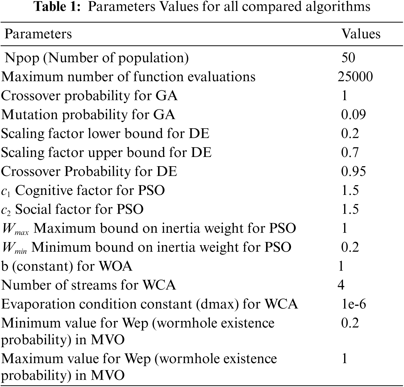
The following conditions are assumed:

1.    To terminate the algorithms, the maximum number of function evaluations is assumed [55].

2.    To handle the constraints, the parameter used in the ALM depends on each example.

3.    A total of 25 independent runs are conducted, and the best results are recorded throughout the process.

4.    The results are compared among the algorithms (GSK, GA, DE, PSO, ALO, WOA, WCA, MOV, and TLBO) and a previous study [16].

5.    The numerical results are shown in terms of maximum (best) objective value, minimum (worst) objective value, average objective value, standard deviation, and coefficient of variation (C.V.).

6.    The results are obtained for the deterministic objective function F(Z).

5.2 Simulation Results

The considered numerical examples are solved by the GSK and other metaheuristic algorithms using MATLAB R2015a on a personal computer having Inter CoreTM i5@2.50GHz processor with 4 GB RAM. To fair comparisons and obtain the optimal global solutions, the examples are solved by LINGO 11.0 and the obtained results of each example are presented in Tabs. 2–4.

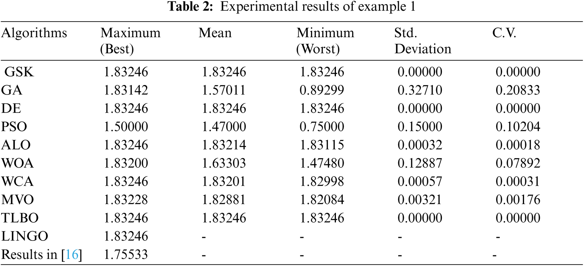
The results of example 1 depict that all the algorithms can find a feasible solution to the problem. GSK, DE, and TLBO obtained the solutions equal to the optimal global solution (F(z)=1.83246) with a minimum standard deviation. The convergence graph of the GSK algorithm with other metaheuristic algorithms is presented in Fig. 3 in which the comparison is shown among the GSK and other algorithms. The convergence graph shows that GSK has the best convergence as compared to the other algorithms. Also, the average elapsed time taken by the GSK algorithm is less than others, which is presented in Fig 6. Moreover, the results obtained by metaheuristic algorithms are much better than the results in the literature (Charles et al. [16]) except for the PSO algorithm. Therefore, the values of decision variables obtained by GSK algorithm are γ1=1.83246, γ2=0, z1=0.202324, z2=0.165433 and the values of the constraints are [−0.5901, −5.9157e−07, −0.4956, −0.5974], that describes the feasibility of the solutions.

Figure 3: The convergence graph for the solution of Example 1

For the solution of example 2, the results are presented in Tab. 3. It indicates that the solutions obtained by GSK, DE, and TLBO are equal to optimal solution with zero standard deviation, which implies that these are efficient algorithms to solve the problem. The obtained results are better than the results in (Charles et al. [16]). Moreover, the computational time is also noted throughout the process. The average elapsed time taken by all algorithms is shown in Fig. 6, which establishes that the GSK algorithm takes less computational time as compared to others. Also, Fig. 4 shows the convergence graph of the GSK algorithm with other algorithms. To show the feasibility of the solutions, the values of the constraints are [0, −2.7569e−06, −1.9445, −0.0536, −3.9992] and the values of the decision variables are γ1=15.22559, γ2=0, γ3=0, z1=0, z2=1.424836, z3=1.681578 that are obtained by GSK algorithm.

Similarly, example 3 is also solved by the GSK algorithm and the other algorithms. The results are shown in Tab. 4 in terms of maximum (best), minimum (worst) and average objective value with their standard deviations and coefficient of variation. All algorithms GSK, GA, DE, PSO, WOA, ALO, WCA, MVO, and TLBO can find the solution, but GSK and ALO algorithm find the optimal solution, which has a 0\% difference from the optimal global solution. The objective function value in (Charles et al. [16]) is 3.6584 which is 53.5\% of the global optimal solution (7.8808). The convergence graph of example 3 by GSK and other algorithms is shown in Fig. 5. The average computational time is presented in Fig. 6, which indicates that the GSK algorithm takes very less computational time. The results obtained by GSK algorithm are: Objective function value=7.8808, value of the decision variables γ1=0, γ2=7.88078, z1=2.4, z2=0, z3=0 and the value of the constraints are [6.7823e−05, −14.2167,0].

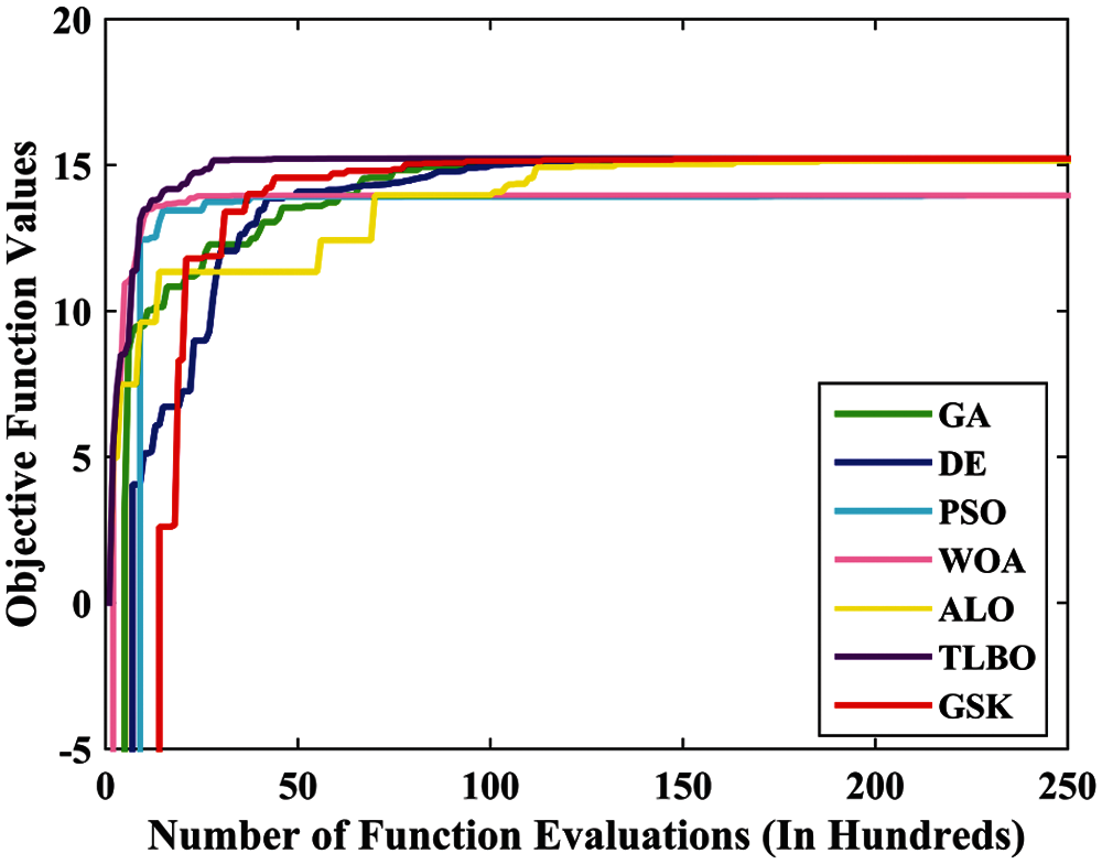
Figure 4: The convergence graph for the solution of Example 2

5.3 Statistical Analysis

To validate the results obtained from the GSK and other algorithms, two non-parametric statistical tests i.e., Friedman test and Wilcoxon signed rank test are performed using IBM SPSS 20.

5.3.1 Friedman Test

To compare the performance of algorithms simultaneously, the Friedman test is conducted by calculating their mean ranks. The null hypothesis is “There is no significant difference among the performance of the algorithms” whereas the alternative hypothesis is “There is significant difference among the performance of the algorithms”. Using the Friedman test, the mean rank is obtained for each example and the acquired results are shown in Tab. 5. According to obtained mean ranks, the ranks are assigned to the algorithms. The high ranks are assigned to the larger value of mean rank and higher ranks indicate the better performance of the algorithm. The same is shown in Fig. 7 for each example. From Tab. 5, it can be observed that the GSK algorithm obtains first rank among others for each example. Moreover, it is noted that all the algorithms have significant differences at the 5\% level (p-value = 0.00 < 0.05) therefore, to check the pairwise comparison, the Wilcoxon signed rank test is also performed.

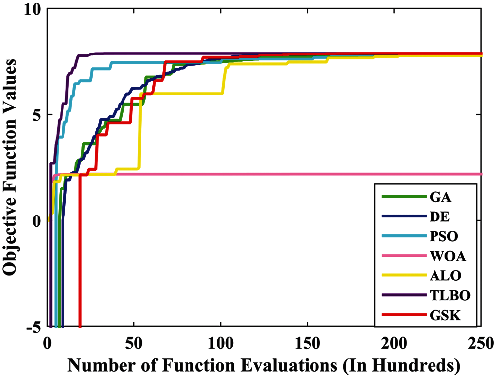
Figure 5: The convergence graph for the solution of Example 3

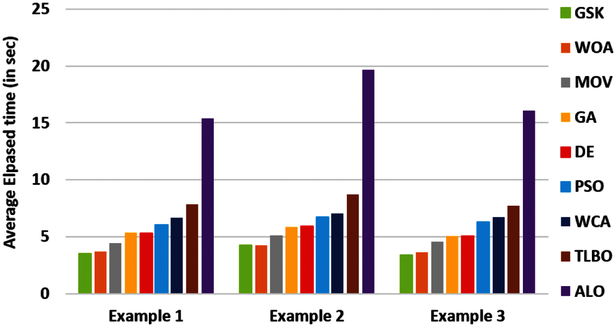
Figure 6: Average Elapsed time of example 1, 2 and 3 for all algorithms

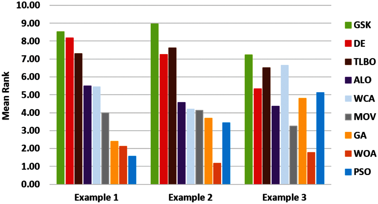
Figure 7: The mean ranks of the algorithms obtained by Friedman test

5.3.2 Wilcoxon Signed Rank Test

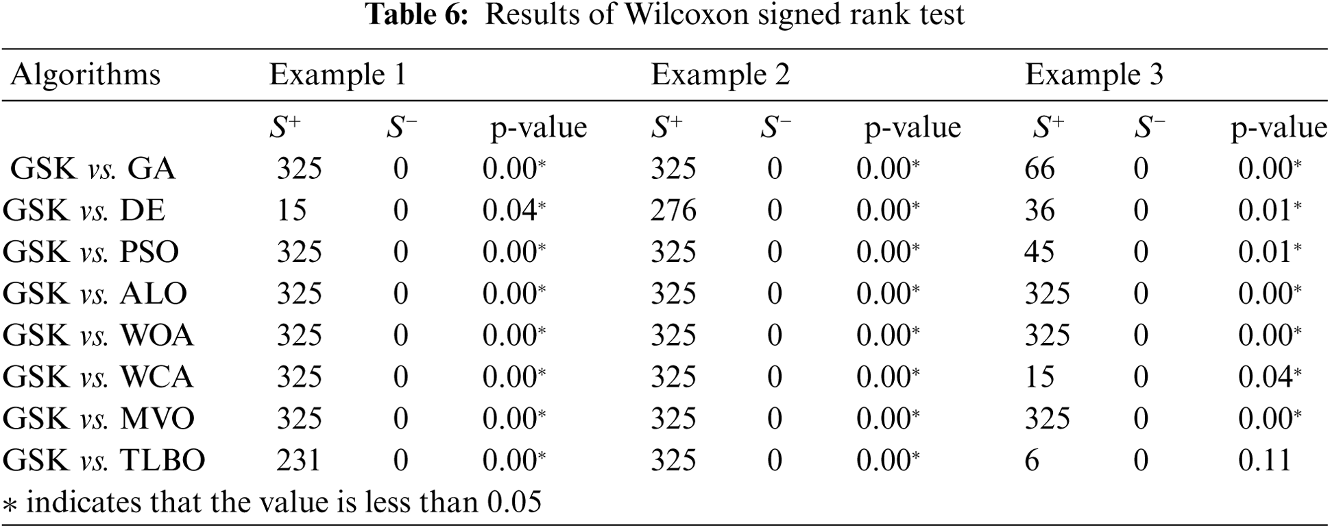
To check the pairwise comparison between the algorithms (GSK vs. GA, GSK vs. DE, GSK vs. PSO, GSK vs. ALO, GSK vs. WOA, GSK vs. WCA, GSK vs. MVO and GSK vs. TLBO), Wilcoxon signed-rank test is performed at the 5\% level of significance. The obtained results are presented in Tab. 6, in which S+, S− denote the sum of positive ranks and negative ranks, respectively. From Tab. 6, it can be observed that the GSK algorithm obtains a higher S+ value than S− for every pairwise comparison. As obtained p−value <0.05, it can be observed that the GSK algorithm performs better when compared to all other algorithms.6.

6  A Case Study

This section contains a case study based on a stochastic transportation problem. The transportation problem is considered with cost objective function in which the main aim is to minimize the total transportation cost and find the total transportation time in Tab. 7.

A cement company transports cement from its 4 distributors (source locations) to 5 retailers (destination locations) with 2 conveyances. In this problem, two categories of transportation cost are asummed: direct costs and fixed costs. The direct cost is paid according to per unit of the transport product and the fixed cost will be charged if the transportation facility occurs between source locations to destination locations. Mathematically, the fixed cost can be formulated by introducing the variables as:

Thus, the total transportation cost can be calculated as

Cost=fcost=∑i=14⁡∑t=15⁡∑k=12⁡(αitkzitk+βitky(zitk))(28)

Also, the total transportation time will be minimized when the transportation activity holds between ith source locations to tth destination locations. Thus, the objective function for the total transportation time can be formulated as

Time=ftime=∑i=14⁡∑t=15⁡∑k=12⁡(ξitky(zitk))(29)

In the classical transportation problem, the data is already known to the decision maker but in real-world problem, the data cannot be obtained in advance. It can be obtained by statistical experience or observed from a previous activity. Hence, the parameters of the problem; ai, bt, qk, αitk, βitk, ξitk are treated as random variables. Therefore, the problem becomes a solid stochastic fixed charge transportation problem (SSFCTP). The mathematical model of the SSFCTP can be formulated as:

minfcost=∑i=14⁡∑t=15⁡∑k=12⁡(αitkzitk+βitky(zitk))(30)

subject to

P(∑t=15⁡∑k=12⁡zitk≤ai)≥γi;i=1,2,3,4(31)

P(∑i=14⁡∑k=12⁡zitk≥bt)≥ηt;t=1,2,3,4,5(32)

P(∑i=14⁡∑t=15⁡zitk≤qk)≥ζk;t=1,2(33)

zitk≥0;y(zitk)=0or1;foreveryi,t,k(34)

where, γi, ηt, ζk are probability confidence levels.

In order to obtain the solution of the problem, the usual procedure cannot be applied. Since the parameters in the objective functions are random variables, the expected minimization model is used to obtain the optimal solution and the chance constrained technique is applied to the probabilistic constraints. The data used for the said problem is taken from Yang et al. [3].

The problem is solved by the GSK and the other algorithms (TLBO, DE, WCA, GA, MVO, WOA). The independent runs for every algorithm are taken to be 15 and, the results are noted throughout the process. The obtained solutions are shown in Tab. 8. It can be observed that the GSK algorithm gives the lowest transportation cost (fcost=1360.4) as compared to the other algorithms. In the case of average cost, the GSK algorithm has the minimum average cost relative to the other algorithms. The minimum and average transportation costs are also presented in Fig. 8 which describes that the GSK algorithm is more efficient in comparison with others. The corresponding total transportation time taken by all transportation activities is ftime=42 hours and the optimal transportation plan is: z112=0.03, z121=0.02, z141=0.06, z212=27.57, z221=27.67, z222=18.36,z241=0.02, z442=34.45 and all other decision variables are zero.

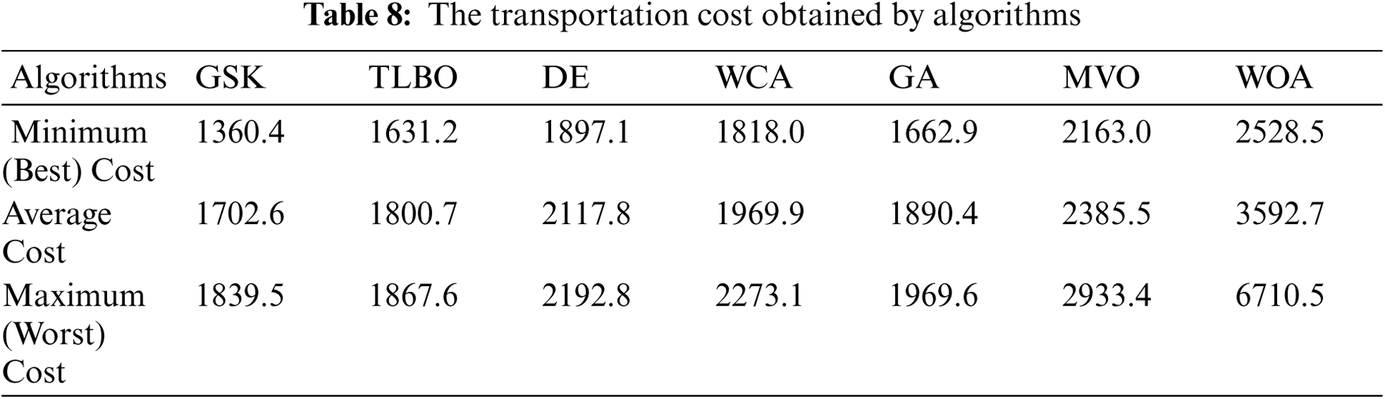
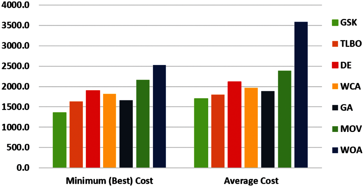
Figure 8: The average and minimum transportation cost

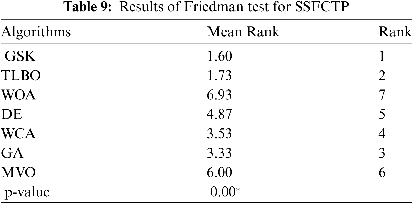
To validate the efficiency and robustness of the GSK algorithm, Friedman Test and Wilcoxon signed-rank test are performed. The obtained results from the tests are shown in Tabs. 9 and 10 respectively. To check the difference among all the algorithms, the Friedman test is applied and it is observed that they are significantly different at (5\%) level. To know the pairwise comparison between the GSK algorithm and all other considered algorithms, Wilcoxon signed-rank test is performed. It can be observed that the GSK algorithm is significantly different when compared to other algorithms at the (5\%) level except for the TLBO algorithm.

7  Results Analysis

From the experimental results, it can be observed that the GSK algorithm performs better in all SFPP examples in terms of convergence, robustness and ability to find the optimal solutions.

In example 1, ALO, PSO, WOA algorithms have premature convergence and do not find the optimal solution of the problem. While GSK algorithm has a fast convergence speed and does not trap into local optima due to its good exploration and exploitation quality. It explores the search space efficiently and effectively and converges to the optimal solution. Moreover, the GSK algorithm proves its robustness quality by obtaining zero standard deviation in all the test examples of SFPP. In case of other algorithms, the techniques do not converge to the optimal solution in every simulation. Also, due to two main pillars of the GSK algorithm i.e., junior and senior gaining sharing stage, the algorithm can find the optimal solution with great convergence. Hence, it can be concluded that the GSK algorithm is a very effective approach to solve the SFPP.

In addition, the GSK algorithm shows promising results in comparison with other metaheuristic algorithms. While other algorithms are not even able to find the optimal solution to the SFPP problem, GSK algorithm convergences to the optimal solution at an early stage of the optimization process. It makes a proper balance between its exploration and exploitation characteristics and finds the solution. Moreover, it consumes very less computational time which is an important characteristic to find the optimal solution. Statistically, it is also shown that the GSK algorithm presents significantly better results as compared to other algorithms by applying statistical tests.

Moreover, based on the results of the stochastic transportation problem, all algorithms other than the GSK did not perform well and also did not obtain the minimum transportation cost of the problem. However, the GSK algorithm obtained the minimum transportation cost and transportation time of the problem, this proves its efficiency to solve real-world problems. Thus, it can be used to solve all optimization problems (unconstrained, constrained and multi-objective) with both discrete and continuous spaces. It is considered a general-purpose algorithm and easy to understand and implement.

8  Concluding Remarks

This paper describes an application of a recently developed gaining sharing knowledge-based algorithm (GSK) to stochastic programming. GSK algorithm is a metaheuristic algorithm which is based on the human activity of gaining and sharing knowledge. To check the performance of the algorithm in terms of convergence and finding the optimal solution, GSK is applied to stochastic fractional programming problems with three different types of numerical examples. For comparative assessment, metaheuristic algorithms from each category, such as GA and DE from evolutionary algorithms; PSO, ALO, and WOA from swarm-based algorithms; WCA and MVO from physics-based algorithm; and TLBO from human-based algorithms are considered.

From the comparative results, it can be concluded that the GSK algorithm performs better than other algorithms. It converges to the optimal solution rapidly and takes less computational time. The obtained results are also compared with the global optimal solution and results from a previous study. For a fair comparison, non-parametric statistical tests (Friedman test and Wilcoxon signed-rank test) are conducted at 5\% level of significance and the GSK algorithm proves that it is significantly different from other algorithms and outperforms them.

Besides, a solid stochastic fixed charge transportation problem, a real-world application of stochastic programming, is studied under a stochastic environment, in which all parameters of the problem are treated as random variables. The main objective of the problem is to find the optimal transportation plan which has minimum transportation cost and minimum transportation time, satisfying all the constraints. Metaheuristic algorithms are applied to the problem and solutions are obtained. From the obtained results, it is observed that the GSK algorithm gives the minimum transportation cost (fcost=1360.4) and minimum transportation time (ftime=42) as compared to other algorithms in less computational time.

From these results, it can be concluded that the GSK algorithm performs significantly better than other metaheuristic algorithms. It is highly noted that the empirical analysis of this study may differ on another benchmark set or real-world problems according to the no-free-lunch theorem.

Acknowledgement: The authors would like to thank the Editor and the reviewers for their valuable suggestions, that helped us to improve the quality of the paper.

The authors present their appreciation to King Saud University for funding this work through Researchers Supporting Project Number (RSP-2021/305), King Saud University, Riyadh, Saudi Arabia.

Funding Statement: The research is funded by Researchers Supporting Program at King Saud University, (Project# RSP-2021/305).

Conflicts of Interest: The authors declare that they have no conflicts of interest to report regarding the present study.

References

 1.  Z. Qin, “Uncertain random goal programming,” Fuzzy Optimization and Decision Making, vol. 17, no. 4, pp. 375–386, 2018. [Google Scholar]

 2.  S. S. Rao, Engineering Optimization: Theory and Practice, John Wiley & Sons, Hoboken, New Jersey, USA, 2019. [Google Scholar]

 3.  L. Yang and Y. Feng, “A bicriteria solid transportation problem with fixed charge under stochastic environment,” Applied Mathematical Modelling, vol. 31, no. 12, pp. 2668–2683, 2007. [Google Scholar]

 4.  M. Alizadeh, J. Ma, N. Mahdavi-Amiri, M. Marufuzzaman and R. Jaradat, “A stochastic programming model for a capacitated location-allocation problem with heterogeneous demands,” Computers & Industrial Engineering, vol. 137, pp. 106055, 2019. [Google Scholar]

 5.  Y. Zhang, X. Li and S. Guo, “Portfolio selection problems with markowitz's mean–variance framework: A review of literature,” Fuzzy Optimization and Decision Making, vol. 17, no. 2, pp. 125–158, 2018. [Google Scholar]

 6.  X. Zhang, S. Huang and Z. Wan, “Stochastic programming approach to global supply chain management under random additive demand,” Operational Research, vol. 18, no. 2, pp. 389–420, 2018. [Google Scholar]

 7.  F. Murphy, S. Sen and A. Soyster, “Electric utility capacity expansion planning with uncertain load forecasts,” IIE Transactions, vol. 14, no. 1, pp. 52–59, 1982. [Google Scholar]

 8.  Z. Hu and G. Hu, “A multi-stage stochastic programming for lot-sizing and scheduling under demand uncertainty,” Computers & Industrial Engineering, vol. 119, pp. 157–166, 2018. [Google Scholar]

 9.  H. Ke, W. Ma and J. Ma, “Solving project scheduling problem with the philosophy of fuzzy random programming,” Fuzzy Optimization and Decision Making, vol. 11, no. 3, pp. 269–284, 2012. [Google Scholar]

10. B. A. Foued and M. Sameh, “Application of goal programming in a multi-objective reservoir operation model in Tunisia,” European Journal of Operational Research, vol. 133, no. 2, pp. 352–361, 2001. [Google Scholar]

11. A. Baykasoglu and T. Gocken, “Multi-objective aggregate production planning with fuzzy parameters,” Advances in Engineering Software, vol. 41, no. 9, pp. 1124–1131, 2010. [Google Scholar]

12. E. Nikzad, M. Bashiri and F. Oliveira, “Two-stage stochastic programming approach for the medical drug inventory routing problem under uncertainty,” Computers & Industrial Engineering, vol. 128, pp. 358–370, 2019. [Google Scholar]

13. V. Charles and D. Dutta, “Linear stochastic fractional programming with branch-and-bound technique,” in Proc. of the National Conf. on Mathematical and Computational Models, Coimbatore, India, Allied Publishers, pp. 131, 2001. [Google Scholar]

14. V. Charles, D. Dutta, and K. A. Raju, “Linear stochastic fractional programming problem,” in Proc. of the Int. Conf. on Mathematical Modelling, University of Roorkee, India, Tata McGraw–Hill, pp. 211–217, 2001. [Google Scholar]

15. V. Charles and D. Dutta, “A method for solving linear stochastic fractional programming problem with mixed constraints,” Acta Ciencia Indica, vol. 30, no. 3, pp. 497–506, 2004. [Google Scholar]

16. V. Charles and D. Dutta, “Linear stochastic fractional programming with sum-of-probabilistic-fractional objective,” Optimization Online, 2005. http://www.optimizationonline.org. [Google Scholar]

17. P. Agrawal, H. F. Abutarboush, T. Ganesh and A. W. Mohamed, “Metaheuristic algorithms on feature selection: A survey of one decade of research (2009–2019),” IEEE Access, vol. 9, pp. 26766–26791, 2021. [Google Scholar]

18. A. W. Mohamed, A. A. Hadi and A. K. Mohamed, “Gaining-sharing knowledge based algorithm for solving optimization problems: A novel nature-inspired algorithm,” International Journal of Machine Learning and Cybernetics, vol. 11, pp. 1501–1529, 2020. [Google Scholar]

19. O. B. Haddad, M. Moravej and H. A. Loáiciga, “Application of the water cycle algorithm to the optimal operation of reservoir systems,” Journal of Irrigation and Drainage Engineering, vol. 141, no. 5, pp. 04014064, 2014. [Google Scholar]

20. J. Claro and J. P. de Sousa, “A multi-objective metaheuristic for a mean-risk static stochastic knapsack problem,” Computational Optimization and Applications, vol. 46, no. 3, pp. 427–450, 2010. [Google Scholar]

21. A. Hoff, A. G. Lium, A. Løkketangen, and T. G. Crainic, “A metaheuristic for stochastic service network design,” Journal of Heuristics, vol. 16, no. 5, pp. 653–679, 2010. [Google Scholar]

22. A. W. Mohamed, “An improved differential evolution algorithm with triangular mutation for global numerical optimization,” Computers & Industrial Engineering, vol. 85, pp. 359–375, 2015. [Google Scholar]

23. A. W. Mohamed, “Solving stochastic programming problems using new approach to differential evolution algorithm,” Egyptian Informatics Journal, vol. 18, no. 2, pp. 75–86, 2017. [Google Scholar]

24. A. Ibrahim, H. A. Ali, M. M. Eid and E. S. M. El-kenawy, “Chaotic harris hawks optimization for unconstrained function optimization,” in 2020 16th Int. Computer Engineering Conf. (ICENCOCairo, Egypt, IEEE, pp. 153–158, 2020. [Google Scholar]

25. F. Hernandez, M. Gendreau, O. Jabali and W. Rei, “A local branching metaheuristic for the multi-vehicle routing problem with stochastic demands,” Journal of Heuristics, vol. 25, no. 2, pp. 215–245, 2019. [Google Scholar]

26. I. Sbai, S. Krichen and O. Limam, “Two meta-heuristics for solving the capacitated vehicle routing problem: The case of the Tunisian post office,” Operational Research, pp. 1–43, 2020. [Google Scholar]

27. H. Yahyaoui, I. Kaabachi, S. Krichen and A. Dekdouk, A., “Two metaheuristic approaches for solving the multi-compartment vehicle routing problem,” Operational Research, pp. 1–24, 2018. [Google Scholar]

28. M. A. Abdeljaoued, N. E. H. Saadani and Z. Bahroun, “Heuristic and metaheuristic approaches for parallel machine scheduling under resource constraints,” Operational Research, vol. 20, no. 4, pp. 2109–2132, 2020. [Google Scholar]

29. El-Sayed M. El-kenawy, Hattan F. Abutarboush, Ali Wagdy Mohamed and Abdelhameed Ibrahim, “Advance artificial intelligence technique for designing double T-shaped monopole antenna,” Computers, Materials & Continua, vol. 69, no. 3, pp. 2983–2995, 2021. [Google Scholar]

30. L. Montiel and R. Dimitrakopoulos, “A heuristic approach for the stochastic optimization of mine production schedules,” Journal of Heuristics, vol. 23, no. 5, pp. 397–415, 2017. [Google Scholar]

31. J. Panadero, J. Doering, R. Kizys, A. A. Juan and A. Fito, “A variable neighborhood search sim heuristic for project portfolio selection under uncertainty,” Journal of Heuristics, vol. 26, no. 3, pp. 353–375, 2018. [Google Scholar]

32. N. Kumar, A. Poddar, A. Dobhal and V. Shankar, “Performance assessment of pso and ga in estimating soil hydraulic properties using near-surface soil moisture observations,” Compusoft, vol. 8, no. 8, pp. 3294–3301, 2019. [Google Scholar]

33. El-Sayed M. El-kenawy and Marwa Eid, “Hybrid gray wolf and particle swarm optimization for feature selection,” International Journal of Innovative Computing Information and Control, vol. 16, no. 3, pp. 831–844, 2020. [Google Scholar]

34. E. S. M. El-Kenawy, S. Mirjalili, A. Ibrahim, M. Alrahmawy, M. El-Said et al., “Advanced meta-heuristics, convolutional neural networks, and feature selectors for efficient COVID-19 X-ray chest image classification,” IEEE Access, vol. 9, pp. 36019–36037, 2021. [Google Scholar]

35. M. K. Dhadwal, S. N. Jung and C. J. Kim, “Advanced particle swarm assisted genetic algorithm for constrained optimization problems,” Computational Optimization and Applications, vol. 58, no. 3, pp. 781–806, 2014. [Google Scholar]

36. A. A. Salamai, E. M. El-kenawy and I. Abdelhameed, “Dynamic voting classifier for risk identification in supply chain 4.0,” Computers, Materials & Continua, vol. 69, no. 3, pp. 3749–3766, 2021. [Google Scholar]

37. P. Agrawal, T. Ganesh and A. W. Mohamed, “A novel binary gaining–sharing knowledge-based optimization algorithm for feature selection,” Neural Computing and Applications, vol. 33, no. 11, pp. 5989–6008, 2020. [Google Scholar]

38. P. Agrawal, T. Ganesh and A. W. Mohamed, “Chaotic gaining sharing knowledge-based optimization algorithm: An improved metaheuristic algorithm for feature selection,” Soft Computing, vol. 25, pp. 1–24, 2021. [Google Scholar]

39. P. Agrawal, T. Ganesh and A. W. Mohamed, “Solving knapsack problems using a binary gaining sharing knowledge-based optimization algorithm,” Complex & Intelligent Systems, vol. 2021, pp. 1–21, 2021. [Google Scholar]

40. P. Agrawal, T. Ganesh, D. Oliva and A. W. Mohamed, “S-shaped and V-shaped gaining-sharing knowledge-based algorithm for feature selection,” Applied Intelligence, vol. 2021, pp. 1–32, 2021. [Google Scholar]

41. J. H. Holland, “Genetic algorithms,” Scientific American, vol. 267, no. 1, pp. 66–73, 1992. [Google Scholar]

42. R. Storn and K. Price, “Differential evolution–a simple and efficient heuristic for global optimization over continuous spaces,” Journal of Global Optimization, vol. 11, no. 4, pp. 341–359, 1997. [Google Scholar]

43. R. Eberhart and J. Kennedy, “Particle swarm optimization,” in Proc. of the IEEE Int. Conf. on Nueral Networks, Citeseer, vol. 4, pp. 1942–1948,. 1995. [Google Scholar]

44. S. Mirjalili, and A. Lewis, “The whale optimization algorithm,” Advances in Engineering Software, vol. 95, pp. 51–67, 2016. [Google Scholar]

45. S. Mirjalili, “The ant lion optimizer,” Advances in Engineering Software, vol. 83, pp. 80–98, 2015. [Google Scholar]

46. H. Eskandar, A. Sadollah, A. Bahreininejad and M. Hamdi, “Water cycle algorithm–a novel metaheuristic optimization method for solving constrained engineering optimization problems,” Computers & Structures, vol. 110, pp. 151–166, 2012. [Google Scholar]

47. S. Mirjalili, S. M. Mirjalili and A. Hatamlou, “Multi-verse optimizer: A nature-inspired algorithm for global optimization,” Neural Computing and Applications, vol. 27, no. 2, pp. 495–513, 2016. [Google Scholar]

48. R. V. Rao, Teaching-Learning-Based Optimization Algorithm, Springer, pp. 9–39, 2016. [Google Scholar]

49. D. R. Mahapatra, S. K. Roy and M. P. Biswal, “Multi-choice stochastic transportation problem involving extreme value distribution,” Applied Mathematical Modelling, vol. 37, no. 4, pp. 2230–2240, 2013. [Google Scholar]

50. P. Agrawal and T. Ganesh, “Solving transportation problem with stochastic demand and non-linear multi-choice cost,” in AIP Conf. Proc., vol. 2134, pp. 060002, 2019. [Google Scholar]

51. C. A. C. Coello, “Theoretical and numerical constraint-handling techniques used with evolutionary algorithms: A survey of the state of the art,” Computer Methods in Applied Mechanics and Engineering, vol. 191, no. 11–12, pp. 1245–1287, 2002. [Google Scholar]

52. E. Mezura-Montes, Constraint-Handling in Evolutionary Optimization, Springer, Switzerland, vol. 198, 2009. [Google Scholar]

53. K. Deb, “An efficient constraint handling method for genetic algorithms,” Computer Methods in Applied Mechanics and Engineering, vol. 186, no. 2–4, pp. 311–338, 2000. [Google Scholar]

54. A. Bahreininejad, “Improving the performance of water cycle algorithm using augmented lagrangian method,” Advances in Engineering Software, vol. 132, pp. 55–64, 2019. [Google Scholar]

55. M. Črepinšek, S. H. Liu and M. Mernik, “Replication and comparison of computational experiments in applied evolutionary computing: Common pitfalls and guidelines to avoid them,” Applied Soft Computing, vol. 19, pp. 161–170, 2014. [Google Scholar]

This work is licensed under a Creative Commons Attribution 4.0 International License, which permits unrestricted use, distribution, and reproduction in any medium, provided the original work is properly cited.