Computers, Materials & Continua DOI:10.32604/cmc.2022.023286
Article

Computational Algorithms for the Analysis of Cancer Virotherapy Model

Ali Raza1,2,*, Dumitru Baleanu3,4, Muhammad Rafiq5, Syed Zaheer Abbas6, Abubakar Siddique6, Umer Javed8, Mehvish Naz7, Arooj Fatima6, Tayyba Munawar6, Hira Batool6 and Zaighum Nazir6

1Department of Mathematics, Govt. Maulana Zafar Ali Khan Graduate College Wazirabad, 52000, Punjab Higher Education Department (PHED), Lahore, 54000, Pakistan
2Department of Mathematics, University of Sialkot, Sialkot, 51310, Pakistan
3Department of Mathematics, Cankaya University, Balgat, Ankara, 06530, Turkey
4Department of Medical Research, China Medical University, Taichung, 40402, Taiwan
5Department of Mathematics, Faculty of Sciences, University of Central Punjab, Lahore, 54500, Pakistan
6Department of Mathematics, National College of Business Administration and Economics, Lahore, 54660, Pakistan
7Department of Mathematics, COMSATS University Islamabad, Wah Campus, Quaid Avenue, Wah Cantonment, 47040, Pakistan
8Department of Electrical and Computer Engineering, COMSATS University Islamabad, Wah Campus, Quaid Avenue, Wah Cantonment, 47040, Pakistan
*Corresponding Author: Ali Raza. Email: alimustasamcheema@gmail.com
Received: 02 September 2021; Accepted: 09 October 2021

Abstract: Cancer is a common term for many diseases that can affect any part of the body. In 2020, ten million people will die due to cancer. A worldwide leading cause of death is cancer by the World Health Organization (WHO) report. Interaction of cancer cells, viral therapy, and immune response are identified in this model. Mathematical and computational modeling is an effective tool to predict the dynamics of cancer virotherapy. The cell population is categorized into three parts like uninfected cells (x), infected cells (y), virus-free cells (v), and immune cells (z). The modeling of cancer-like diseases is based on the law of mass action (the rate of change of reacting substances is directly proportional to the product of interacting substances). Positivity, boundedness, equilibria, threshold analysis, are part of deterministic modeling. Later on, a numerical analysis is designed by using the standard and non-standard finite difference methods. The non-standard finite difference method is developed to study the long-term behavior of the cancer model. For its efficiency, a comparison of the methods is investigated.

Keywords: Cancer disease; epidemic model; algorithms; stability analysis

1  Literature Survey

Cancer is a disease of abnormal cell growth, and these cells attach to other cells of the body and harm them. It can start in any part of the body. Typically human cells grow and divide to replace old or damaged cells. Still, this process breaks down in a cancer patient, resulting in the formation of irregular or deteriorated cells and new abnormal cells. It includes tumors that may or may not be cancerous. In immunotherapy, we enhance our immune system (defensive system against diseases) by using different substances (body cells or proteins). These substances may destroy cancerous cells or stop the growth of uncontrolled dividing cells. In this technique, medicines are more effective in malignancies than in other cancers. It can be a lifesaver for some victims. This technique is not suitable for everyone. In general, fifteen to twenty out of a hundred people respond. Virotherapy is a biotechnology-based treatment that transforms viruses into therapeutic agents by reprogramming them to cure diseases. As a result, oncolytic virotherapy is now considered to be generally safe. Possible safety concerns that have yet to be identified or demonstrated cannot be ruled out. It is one of the most prominent therapies in growing research for mesothelioma because of its capacity to select and kill malignant cells natively. Selmi et al. [1] in 2020, proposed an analysis to numerically feature radio heat therapy’s efficacy in curing liver tumors. Zheng [2], in 2020, suggested a model for cancer cells and their spread in the body. In 2020, Yousef et al. [3] proposed an NTIE model to analyze chest cancer by regulating nourishment, body protection, and medication. Koziol et al. [4] in 2020 have proposed an ordinary differential equation model for dynamics of cancer growth. Lestari et al. [5] in 2019, developed an ETM model to study the improvement in cancer cells undergoing chemotherapy. Weerasinghe et al. [6] in 2019, presented a dynamical model for the explanation of plasticity behavior of cancer cells. In 2019, Hillen et al. suggested a stochastic model for the spreading of disease in the body. They also calculate the reproduction number and use mice for their experiments [7]. In 2019, Unni et al. [8] presented the TNDLMI model to study the change in behavior of tumors due to intake of medicine by the patient. Malini et al. [9] in 2019 proposed a dynamic model to check the effectiveness of the drug on cancer cells. Ray et al. [10] in 2019, developed guided machine learning techniques for classifying benign and malignant breast cancers. Oyelami [11], in 2018, proposed a mathematical model for cancer cells and the immunization response of the body. In 2018, Alameddine [12] presented a simplified and latest study tool to model cancer systems. In 2016, Baar et al. [13] presented modeling of the malignant tumor by randomizing effect. Pang et al. [14] in 2016, showed a dynamic model for target cancer cells by using different techniques of treatment. Xu et al. [15] in 2016, proposed a delay model for cancer cells and their treatment with therapy. In 2016, Lorenzo [16] presented Prostate tumor development forming and simulation at the tissue level. Watanabe et al. [17] in 2016, suggested a mathematical model study the cancer lump progress with ray’s effect. In 2014, Rihan et al. [18] developed a TCET model to study cancer-protected response DDM model through chemotherapy and ideal switch. Chaplain et al. [19] in 2013, investigated a mathematical model for the explanation of the attack of cancer cells on normal cells. Allegretto [20], in 2006, proposed a mathematical model of cancer unchanging in time. Some well-known models related to cervical cancer and many more are presented in [21–26]. The mathematical techniques are studied to analyze the transmission of infectious diseases [27–36]. Mathematical modeling is one of the essential branches of science to explore real-world problems. In recent history, coronavirus, influenza, dengue, and many more infectious diseases modeled and predicted possible outcomes to overcome them. In the same, we study the dynamics of the cell population in the human body, which means how a cell can be destroyed or save from the infection or which therapy is suitable to control the condition of cells. So, we decided to model the cancer disease analytically and by using computational algorithms. The rest of the paper is organized as follows. In Sections 2 to 4, we investigate thme dynamic analysis of the model. Section 5 explains the well-known numerical methods used in this model. The last two sections present the results, discussion, and conclusion.

2  Formulation of Cancer Model

For any instant t, the cancer model’s parameters and variables listed are as follows: x(t): shows the cancer cells that haven’t been infected, y(t): symbolizes infected cancer cells, v(t): represents free viral cells, z(t): represents immune cells, λ: represents the virus’s growth rate, c: exemplifies the carrying capacity Virus, d: represents the mortality rate, β: represents the rate of oncolytic viral infection in cancer cells, δ: represents the number of infected cells, b: represents particles fired at a burst size, γ: represents the pace at which free virus cells disintegrate, a: shows the fraction of cells that are not infected, it also indicates immunity, μ: reflects immunity in the number of infected cells, k: shows the rate at which a free virus with impunity is eliminated, h2: shows the pace at which an exemption, m1: represents immunity’s rate of stimulation of infected cells, and ρ: represents the rate of immune cell destruction. The governing equations of the model are as follows:

x′(t)=r1−ax(t)v(t)−d1x(t),t≥0.(1)

y′(t)=ax(t)v(t)−cy(t)z(t)−d1y(t)−by(t),t≥0.(2)

v′(t)=by(t)−h2y(t)z(t)−d1v(t)−m1v(t),t≥0.(3)

z′(t)=cy(t)z(t)+h2y(t)z(t)−d1z(t)+m1v(t),t≥0.(4)

2.1 Properties

The feasible region of the model is defined as Υ={(x,y,z,v)ϵR+4:N(t)≤r1d1, x(t) ≥ 0, y(t) ≥ 0, v(t) ≥ 0, z(t) ≥ 0}, N = x + y + v + z.

Lemma 1: The initial values {x(0),y(0),z(0),v(0)}∈Υ, then the solution set {x(t),y(t),z(t),v(t)} is positive of all t≥0.

Proof: From Eq. (1), we have

So, x≥0. All other state variables preserve a positive solution, as desired.

Lemma 2: The solution of the model equation in (1)–(4) are bounded in Υ for all t≥0.

Proof: Firstly, adding the Eqs. (1)–(4) as follows:

where N0 is the initial condition of N,

So, limt→∞SupN(t)≤r1d1. This show that 0≤N≤r1d1 and N = x+y+v+z, then all variable is bounded in Υ.

2.2 Equilibria

There are two steady states of Eqs. (1)–(4), as follows: cancer-free equilibrium (CFE)=(x1,y1,v1,z1)=(r1d1,0,0,0), and cancer existing equilibrium (CEE)=(x∗,y∗,v∗,z∗),

where x∗=r1av∗+d1,y∗=ar1v∗(av∗+d1),v∗=h2βz∗−bβd1+m1,z∗=m1γcβ+h2β−d1.

3  Reproduction Number (R0)

The next-generation matrix method is presented for the system (1–4). We calculate two types of matrices like transmission and transition after assuming the cancer-free equilibrium as follows:

The eigenvalues of the system is as follows:

The spectral radius of the model is denoted by R0=abr1d1(d1+b)(d1+m1).

4  Local Stability

Theorem 1: The disease-free equilibrium of model (1) to (4) is locally asymptotically stable if the reproduction number is less than one and unstable if greater than one.

Proof: To prove the local asymptotically stable cancer-free equilibrium, we take the Jacobian matrix of the cancer model at cancer-free equilibrium.

where, λ1=−d1<0,λ2=−d1<0.

where a0=2d1+b, a1=(d1+b)(d1+m1)−ba(r1d1).

It is clear that both are a0,a1>0, if R0<1, thus we have

So, all eigenvalues are negative. Thus, cancer-free equilibrium is locally stable by using the Routh Hurwitz criteria of 2nd order.

Theorem 2: If the reproduction number is more significant than one, then the cancer existing equilibrium of the model Eqs. (1)–(4) is locally asymptotically stable in Υ.

Proof: The Jacobian matrix at cancer existing equilibrium is as follows:

And, m0=1,m1=A+d1+F−I−B, m2=AF−AB−AI−d1F−DF+BI−FI−CF−DH,m3=ABI−ABF−AFI−ACE−ADH+d1BI−d1BF−d1F1−d1I−d1CE−d1DH+BFI+m1G+CEI−CGH−CEm1−DHF+ACE, m4=ABFI+AGm1+ACEI−ACGH−ADEm1−ADHF+BFTd1+Gd1m1+d1CEI−CGHd1−DEm1d1−DHFd1−ACEI+ACHG.

Here, A=av, B=−d1−b−cy, C=ax, D=−cy, E=b−h2z∗, F=d1+m1

G=−h2y, H=cz+h2z, I=cy−d1+h2y.

By using Routh Hurwitz’s criteria of order 4th,

m0,m1>0, m1m2−m0m3>0, (m1m2−m0m3)(m3)−m12m4>0, m4>0 if RO>1.

Hence, cancer existing equilibrium (CEE) of the given system (1–4) is locally asymptotically stable.

5  Algorithms

In this section, we present the well-known algorithms like Euler, Runge Kutta, and non-standard finite difference for the system (1)–(4) as follows:

5.1 Euler Algorithm

The pseudo-code for the Euler algorithm for the system (1)–(4) is as follows:

Begin:

Declare all constants

Set the step size ‘h.’

Declare arrays for x,y,v,z. The arrays should be able to store 2000 values.

Put initial values for x,y,v,z at index 1 of the corresponding arrays.

Index = 2

For t from 0.1 till t<200

Calculate stage equations

Index = Index + 1

t=t+0.1

End For

Plot required data

end program.

5.2 Runge-Kutta Algorithm

The pseudo-code for the Runge Kutta algorithm for the system (1)–(4) is as follows:

Begin:

Declare all constants

Set the step size ‘h’

Declare arrays for x,y,v,z. The arrays should be able to store 1000 values.

Put initial values for x,y,v,z at index 1 of the corresponding arrays.

Index = 2

For t from 0.1 till t<100

Calculate stage 1 equations

Calculate stage 2 equations

Calculate stage 3 equations

Calculate stage 4 equations

Calculate final stage equations

Index = Index + 1

t=t+0.1

End For

Plot required data

end program.

5.3 Non-Standard Finite Difference Method

The system (1–4) is described under NSFD method is as follows:

xn+1=xn+hy1+ahvn+hd1(5)

yn+1=yn+haxnvn1+ahczn+hd1+hb(6)

Vn+1=vn+hbyn−hh2ynzn1+hd1+hm1(7)

zn+1=zn+hcynzn+hh2ynzn+hm1vn1+hd1(8)

where the time step is represented by h.

5.4 Stability Analysis

Theorem: For any n≥0, the proposed NSFD method is stable if the eigenvalues of the system (5)–(8) lie in the unit circle for R0<1.

Proof: Consider the right-hand sides of the system of Eqs. (5)–(8) as functions A, B, C and D is as follows:

The Jacobian Matrix for the system (5)–(8) is as follows:

The Jacobian matrix at cancer-free equilibrium (CFE) =(r1d1,0,0,0) is as follows:

Lemma 3: For the quadratic equation λ2−P1λ+P2=0, |λi|<1,i=1,2, 3, if and only if the following conditions are satisfied:

(i). 1+P1+P2>0.

(ii). 1−P1+P2>0.

(iii). P2<1.

5.5 Numerical Results

In this section, we investigate the numerical results for the said model with the help of computer software and the scientific literature presented in Tab. 1 as follows:

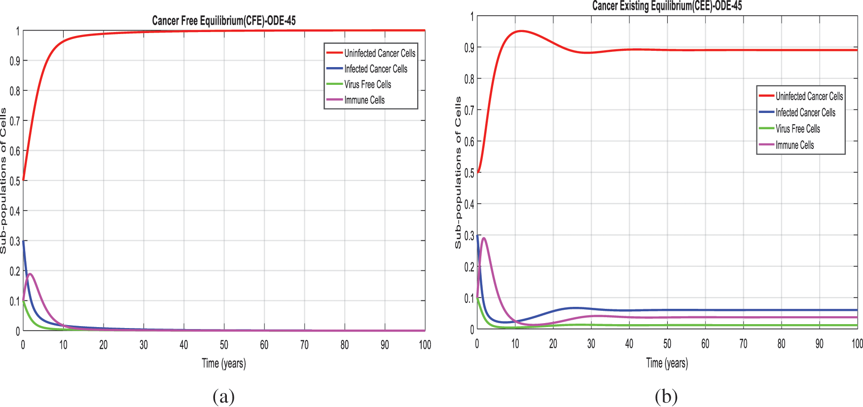
Figure 1: Combined graphical behaviors for CFE and CEE at different subpopulations of the cancer disease (a) Subpopulations for CFE at any time t (b) Subpopulations for CEE at any time t

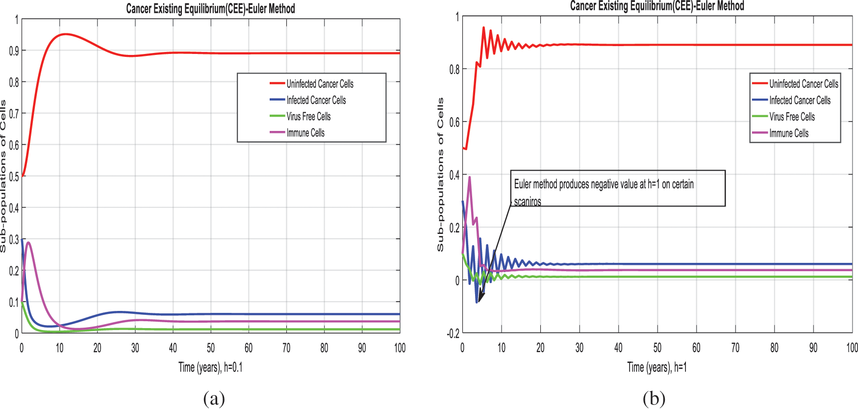
Figure 2: Euler method for the behavior of subpopulations of cells at different time-step sizes (a) Sub-populations of cells at h=0.1 (b) Sub-populations of cells at h=1

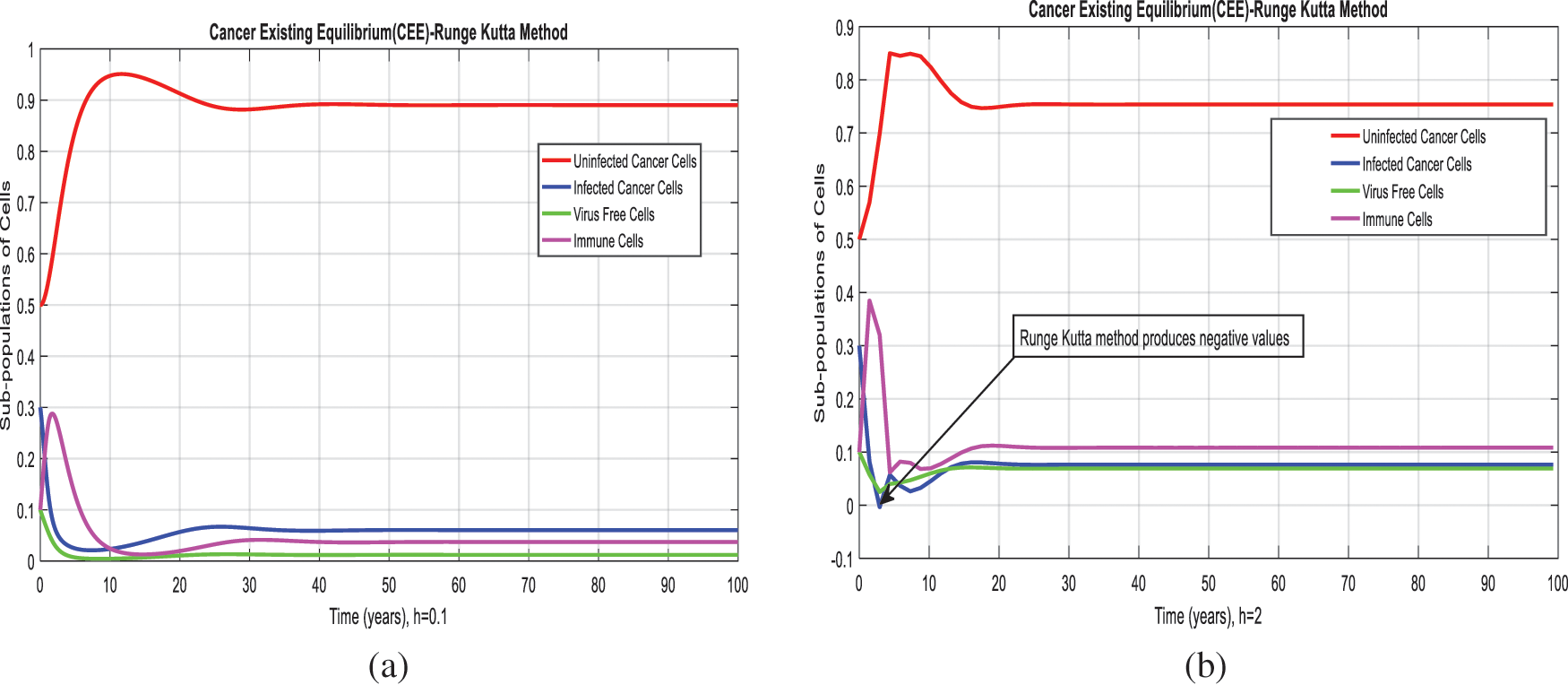
Figure 3: Runge Kutta method for the behavior of subpopulations of cells at different time-step sizes (a) Sub-populations of cells at h=0.1 (b) Sub-populations of cells at h=1

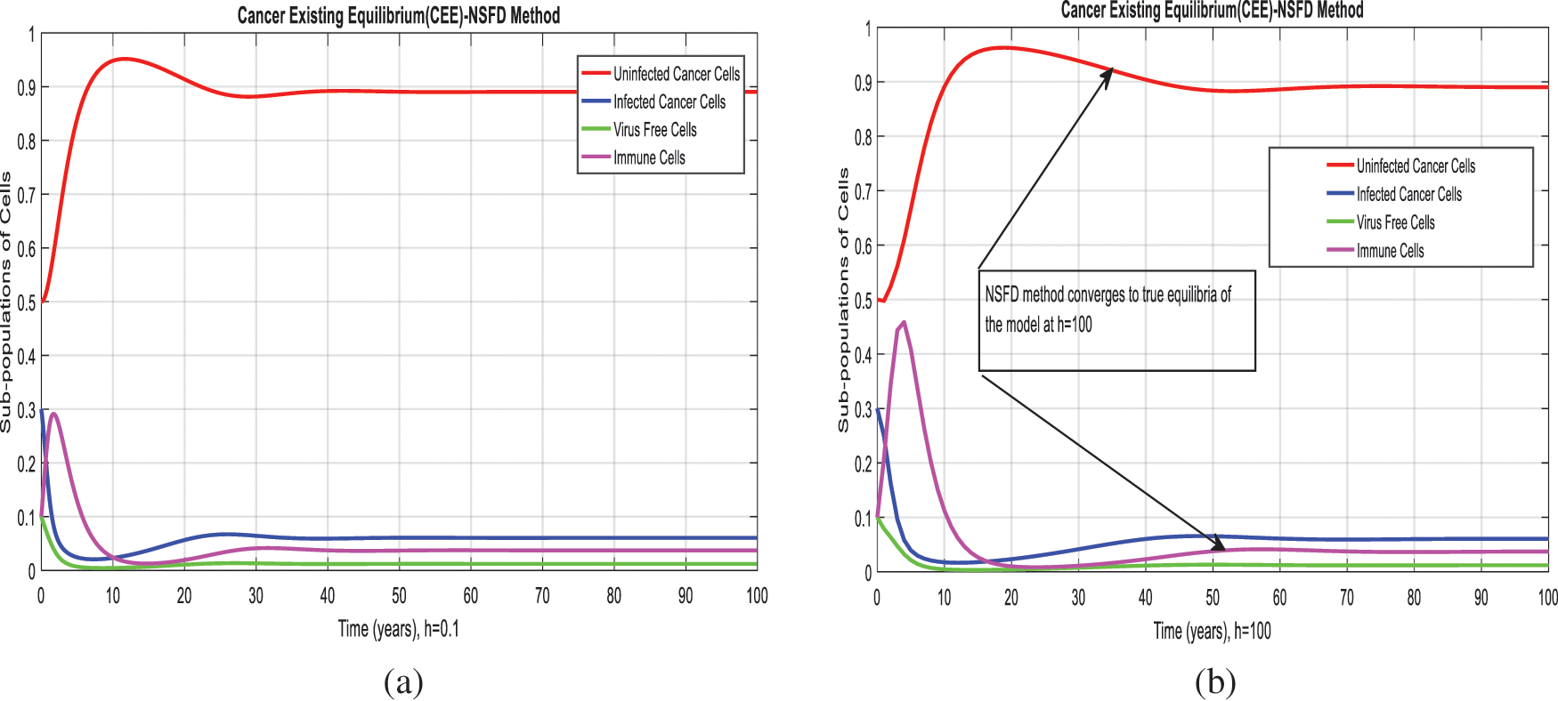
Figure 4: NSFD method for the behavior of subpopulations of cells at different time-step sizes (a) Sub-populations of cells at h=0.01 (b) Sub-populations of cells at h=100

5.6 Comparison Section

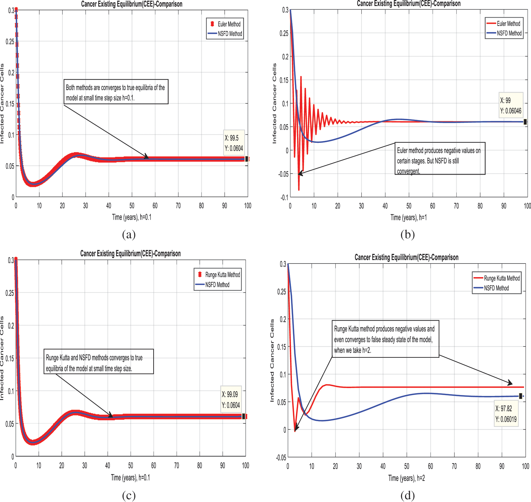
Figure 5: Combined graphical behaviors of NSFD with Euler and Runge Kutta methods at different time-step sizes (a) Infective cancer cells for CEE at h=0.1 (Euler and NSFD) (b) Infective cancer cells for CEE at h=2 (Euler and NSFD) (c) Infective cancer cells for CEE at h=0.1 (Runge Kutta and NSFD) (d) Infective cancer cells for CEE at h=2 (Runge Kutta and NSFD)

6  Results and Discussion

We present the solution to the system (1–4) via Matlab ordinary differential equations-45 at cancer-free and cancer existing equilibria of the model in Figs. 1a, 1b. Also, the solutions of the system via the Euler method at different time step sizes are in Figs. 2a, 2b. The system’s answer via the Runge Kutta method at different time step sizes is in Figs. 3a, 3b. In the same, we plot the solutions of the system (5–8) via the NSFD method in Figs. 4a, 4b. The comparison section in Figs. 5a–5d investigates numerical methods such as Euler and Runge Kutta with NSFD approximations. Here, we observe that Euler and Runge Kutta show negativity and unboundedness and violate the dynamical properties of the model. However, our proposed numerical approximation is reliable, inexpensive, independent of the time step, and an efficient computational method.

7  Conclusion

We here investigated analyses of cancer-like disease via well-known numerical methods. Numerical results of epidemic models are an authentic tool to cross-check the dynamical analysis of the model. For the sake of numerical analysis, Euler, Runge Kutta, and the non-standard finite difference methods (NSFD) are presented. Throughout the study, we observe that Euler and Runge Kutta are time-dependent techniques. Even when we increase the time step duration, these methods violate such dynamic properties as positivity, boundedness, and dynamical consistency. However, NSFD is always concurrent and independent of the size of the time step. Everyone could observe these things from the comparison section. Could extend this idea to different types of disease modeling.

Acknowledgement: We always warmly thanks anonymous referees for their time and valuable comments. Also, thankful to a native speaker who improves the quality of the paper. Thanks, our families and colleagues who supported us morally.

Funding Statement: The authors received no specific funding for this study.

Conflicts of Interest: The authors declare that they have no conflicts of interest to report regarding the present study.

This work is licensed under a Creative Commons Attribution 4.0 International License, which permits unrestricted use, distribution, and reproduction in any medium, provided the original work is properly cited.