Computers, Materials & Continua DOI:10.32604/cmc.2022.023634
Article

Distance Matrix and Markov Chain Based Sensor Localization in WSN

Omaima Bamasaq1, Daniyal Alghazzawi2, Surbhi Bhatia3, Pankaj Dadheech4,*, Farrukh Arslan5, Sudhakar Sengan6 and Syed Hamid Hassan2

1Department of Computer Science, Faculty of Computing and Information Technology, King Abdulaziz University, Jeddah, Saudi Arabia
2Department of Information Systems, Faculty of Computing and Information Technology, King Abdulaziz University, Jeddah, Saudi Arabia
3Department of Information Systems, College of Computer Science and Information Technology, King Faisal University, Saudi Arabia
4Department of Computer Science and Engineering, Swami Keshvanand Institute of Technology, Management & Gramothan, Jaipur, Rajasthan, India
5University of Engineering and Technology, Lahore, Pakistan
6Department of Computer Science and Engineering, PSN College of Engineering and Technology, Tirunelveli, Tamilnadu, India
*Corresponding Author: Pankaj Dadheech. Email: pankajdheech777@gmail.com
Received: 15 September 2021; Accepted: 26 October 2021

Abstract: Applications based on Wireless Sensor Networks (WSN) have shown to be quite useful in monitoring a particular geographic area of interest. Relevant geometries of the surrounding environment are essential to establish a successful WSN topology. But it is literally hard because constructing a localization algorithm that tracks the exact location of Sensor Nodes (SN) in a WSN is always a challenging task. In this research paper, Distance Matrix and Markov Chain (DM-MC) model is presented as node localization technique in which Distance Matrix and Estimation Matrix are used to identify the position of the node. The method further employs a Markov Chain Model (MCM) for energy optimization and interference reduction. Experiments are performed against two well-known models, and the results demonstrate that the proposed algorithm improves performance by using less network resources when compared to the existing models. Transition probability is used in the Markova chain to sustain higher energy nodes. Finally, the proposed Distance Matrix and Markov Chain model decrease energy use by 31% and 25%, respectively, compared to the existing DV-Hop and CSA methods. The experimental results were performed against two proven models, Distance Vector-Hop Algorithm (DV-HopA) and Crow Search Algorithm (CSA), showing that the proposed DM-MC model outperforms both the existing models regarding localization accuracy and Energy Consumption (EC). These results add to the credibility of the proposed DC-MC model as a better model for employing node localization while establishing a WSN framework.

Keywords: Wireless sensor network; resource optimization; routing; distance matrix; Markov chain

1  Introduction

The overwhelming amount of networking components has boosted the use of Wireless Sensor Networks (WSN) in a wide range of disciplines, including medical fields, industrial control, home automation and environmental monitoring [1,2]. The localization technology has gained its importance in WSN since the sensor node's physical location is vital in WSN-based applications. The anchor nodes are special kind of network nodes, which has definite positions and all the other nodes, which don't have a defined location, calculates its location, by interacting with these anchors [3]. The accuracy of localization algorithms is critical since it has a direct impact on the performance of networks. To improve the services available in the network, an efficient localization technique is a crucial factor, and so it attracted many researchers to the field of sensor node localization [4]. Localization can be accomplished in two ways: (i) distributed localization, whereby each node can locate its position by itself, and (ii) centralized localization, where the data from the node are sent to a centralized unit, which processes the data to extract location information.

Further, the localization problems in WSNs are divided into two classes: location estimation and location detection. In local estimation techniques, the un-localized nodes send the signals to the anchor node. Based on the signals received, the anchor nodes calculate the location of the un-localized node. In some applications, for example, consider a fire protection network in a building; within each room, one node is installed, and all anchors are aware of its location, but whether the node is active or not is not known. In this case, every anchor node receives the noise signal if there is no transmission from the node, and each anchor will receive a faded signal along with noise if there is a transmission from the node. Localization of SN falls under the range-based algorithm [5–7] or range free algorithm [8–10]. The location detection algorithm determines whether the node is operational or not based on the signal received from the nodes. Home automation, inventory tracking, patient monitoring and forest fire tracking are just a few areas where WSNs have been employed for localization. WSN with fusion centers [11] has a similar architecture to localization problems where all the necessary processing occurs at a central node. WSNs without a fusion Centre (totally dispersed networks) benefit from being more resilient to node failures since they can operate independently without a single node to manage the whole network. Sensors in highly distributed networks cooperate with their neighbours by exchanging information locally to agree on a global function of initial measurements [12].

This paper proposes the DM-MC approach for performing sensor node localization and resource optimization in WSN to achieve efficient routing. Distance Matrix and Markov Chain model are used to implement the proposed DM-MC method. To decrease the time taken to send sensed data, the locations of SN are first identified using parameter determination. The distance matrix uses multiple iterations to achieve both global and local convergence. After that, the Markov Chain of energy efficiency model is utilized in SN to handle both interference reduction and energy optimization. Multiple user models are used to control the offset of interference reduction and energy usage. In order to offer resource-optimized routing and data acquisition in WSN, the sequence is iterated.

Other sections are arranged as follows: Section 2 deals with authors engaged in a similar framework. The Section 3 gives the readers an understanding of the problem by providing preliminaries. Section 4 presents the proposed methodology followed by the simulation of the results in Section 5, and the conclusion is shown in Section 6 of the article.

2  Literature Review

Nodes estimate their positions in the networks by using the pairwise distance measurements between their neighbours. To tackle localization difficulties because of pairwise distance measurements, several centralized techniques have been developed. Author [13] used convex optimization and semi-definite programming to solve the localization problem. The network's interconnection is represented in the optimization problem by using convex localization constraints. To make the restrictions tight enough for the technique to process, the anchor nodes must be put on the external periphery, particularly at the corners. If every one of the anchors is in the network internally, outer node location estimation can readily converge toward the center resulting in substantial errors. By giving importance to the constraints based on non-convex inequality, Xiang et al. [14] expanded Doherty's technique. Moussa et al. [15] used a gradient search strategy to improve Biswas’ method. A maximum probability estimation is provided by Moses et al. [16]. A nonlinear least-squares method is used to find the solution since the localization estimation problem is an unrestricted optimisation problem. Zhang et al. [17] introduced a Genetic Algorithm based on Localization (GAL).

The optimization problem of localization was stated as a minimum Mean-Squared Error (MSE) problem by Molina et al. 2011 [18]. The precision has improved due to the communication range constraint. However, the inconsistency problem in multilateration has yet to be solved. To rectify the mistake in multilateration, Liu et al. [19] utilized the expansion of Taylor series with a weighting approach. But the computational complexity, on the other hand, is significantly larger. DV-Hop localization has recently incorporated bio-inspired computing with rapid convergence; however, offline computational tools are required to support these approaches. In Bayne et al. 2017 [20] and Minu et al. 2015 [21], a Distance Vector-Hop (DV-Hop) weighting method is presented based on Received Signal Strength Indicator (RSSI). The basic idea is to use weighted data to determine average hop distance based on the received signal power level. Even though the technique increases the measurement of average distance, it is not suited for anisotropic networks with frequent detoured pathways. Wang et al. [22] used a mobile agent to collect data along a predetermined path.

In their study, Xu et al. 2019 [23] suggest a nonlinear optimization problem using the bio-inspired strategy for tackling the localization problem in WSN. Clonal Selection Technique (CST), a population-based optimization algorithm inspired by artificial intelligence, is used to locate nodes in a WSN scenario. Bradai et al. [24] published in 2018 focuses on issues in node WSN. A detection and estimation framework are used to explain WSN localization issues. A cooperative approach is utilized to locate nodes at unknown locations by utilizing sensors with known positions. For WSN, [25] present a 3D localization technique based on RSSI and Time of Arrival (TOA) data. For WSN, the first addition to the proposed 3D localization technique was an anchor node that moves as per a Gauss–Markov 3D mobility model. A novel approach for spatial routing is proposed and implemented by Amri et al. 2019  [26]. A weighted centroid localization methodology is used in the proposed mechanism to determine the locations of un-localized nodes utilizing fuzzy logic. In order to do this, the fuzzy localization technique uses wireless flow measurements to determine the distance between both the anchor and the un-localized nodes.

3  Preliminaries

To make the deployment of the following algorithm easier, we will now quickly outline the underlying idea of distance measuring in WSNs [27,28].

3.1 Non-Anchor Nodes’ Distance Resolving

To begin, the anchor nodes are labelled. The position of the anchor nodes is well defined, whereas nodes with uncertain placements are labelled as un-localized or non-anchor nodes. Un-localized and anchor nodes interact with one another in a WSN to estimate non-anchor node positions. Consider a WSN with N anchor nodes N1, N2, N3,… Nn and the kth node Nk in the N-dimension may be represented using the estimated vector, Eq. (1)

Vi={Vi1,Vi2,Vi3,…,Vin}T,(1)

where Vij indicates the measurement estimation that exists between nodes Ni and Nj, and Viidenotes the measurement estimation that exists between nodes Ni and Ni, and ViiT stands for the linear transformation function. = 0. The embedded N-dimension is thus described by the estimated matrix in the below Eq. (2).

V=[V1,V2,V3,…,Vn](2)

The node distances between the nodes are given as, Eq. (3)

Di={di1,di2,di3,…,din}T(3)

where dij is the distance between the two nodes Ni and Nj, and dii is the distance between the two nodes Ni and Ni, according to Eq. (1), and dii = 0. As a result, the distance matrix is shown as Eq. (4)

D=[D1,D2,D3,…,Dn](4)

Consequently, we can choose the best linear transformation to create a mapped link between the estimate and distance matrices. Respectively, every non-anchor node containing a projected vector has a matching vector distance that may be used to compute its coordinate. A minor variance resolution technique is used to identify each row of the function T, which is set up as a N × N matrix, Eq. (5)

ei=∑k=1n⁡(dik−tivk)2=‖diTtiV‖2(5)

The row of the matrix is given as t till the following condition is satisfied, Eq. (6)

[D1,D2,D3,…,Dn]=[V1,V2,V3,…,Vn]T(6)

the matrix T's row vector can be expressed as in Eq. (7)

t1:ti=diTVT(VVT)−1(7)

Together with the matrix as in Eq. (8)

T=DVT(VVT)−1(8)

3.2 Iterative Approach

After obtaining energy and interference data, an iterative method is used to optimize resources in the WSN. A multi-user model with a MCM of SN considers both energy optimization and interference reduction. The activities of nodes are monitored using an iterative method, where a node is either cooperative or non-cooperative. A network is defined by many nodes that each have a set of tasks and responsibilities that are equivalent. The following describes how the iterative method is used in WSN on the MCM of SN.

Gm⟨Ns,SNs,UF⟩(9)

From Eq. (9), Ns indicates the SN in a MCM, s1,s2,s3…sn,SNsdenotes the SN’ plan of action (i.e., strategy), and UF={u1,u2,…,un} denotes the payoff function. After the channel conditions are fixed, high-power SN is dispersed to obtain a higher node utility value, which is represented asui=(i=1,2,…,n). Iterative nodes provide the adequate condition for a network.

Along with their preference, nodes boost their penalty.

The generated payoff functions are used to choose a strategy Si in which the optimal response is given to a reward function chosen by the other sensor nodei−k. The parameter Siis the tactic selected by node i whereas Si−k denotes the strategy taken by other nodes k in the proposed DM-MC technique. As a result, the approach is as follows:

Strategy(S)={si,si−k}(10)

The strategy function ‘Strategy (S)’ is sometimes referred to as strategy profile given in Eq. (10). A set of strategy profiles is used for selecting a strategy profile S. Assume that the given strategy is persistent across all SN. The power is transmitted by all nodes, with low and high range values. The utility function aids in providing node preferences for a certain node, with a greater number for each possible outcome implying that the outcome is more preferred. As a result, both EC and interference reduction are maximized for the resources. The utility function is written as follows,

ui(si,si−k)=B∗RPsizef(δ)(11)

ui(si,si−k) refers to the utility of a sensor node that sends information to other nodes, for a packet size Psize the number of information bits is represented as B, and R indicates the transmission rate in bps through the strategy function. According to Eq. (11), f(δ) is an efficiency function in this case. The efficiency of the receiving node is enhanced by the probable noise ratio, as shown below.

f(δ)=12(2−PE)F(12)

The bit error rate “PE” depends on the channel interference between other nodes available and the channel condition as shown in Eq. (12). For a greater utility function, nodes are dispersed with maximum power. As a result, the Net utility function is used to assess the effectiveness of data transmission. The ‘ui(net)’ net utility function is given below.

ui(net)={ui(si,si−k)−C(si)iftransmittingonottransmitting(13)

The net utility function ‘ui(net)’ is the cost of the functionC(si), which is raised for each increase in transmit power according to Eq. (13). As a result, the cost of energy is compensated by EC, and noise interference channels are avoided. This approach selects a strategy to modify the transmission channel based on the remaining network nodes with the highest energy savings rate. Finally, any communication channel may give the lowest resource usage for efficient energy use and interference reduction. As a result, interference offset and EC are dealt with in WSN to achieve resource-efficient routing and data gathering.

4  Proposed Methodology

This section covers the sensor node localization algorithm's design principles and the placement procedure in detail. The proposed localization technique is divided into four stages: preprocessing, parameter determination, non-anchor localization, and Markov-chain based resource optimization. The WSN is set up to communicate with both anchor and non-anchor nodes. Measurement distances are used to calculate correlated variables’ linear transformation function, distance and estimate matrix. The parameters acquired before are used to locate the non-anchor node. The following sections go through each stage in further depth.

Convergence-based Node Localization, as seen in Fig. 1, aids in improving routing and data collecting efficiency. The use of an iterative technique makes it easier to integrate EC and interference reduction. As a result, the suggested DM-MC technique achieves considerable resource optimization. The next subsections demonstrate preprocessing, parameter determination and resource optimization.

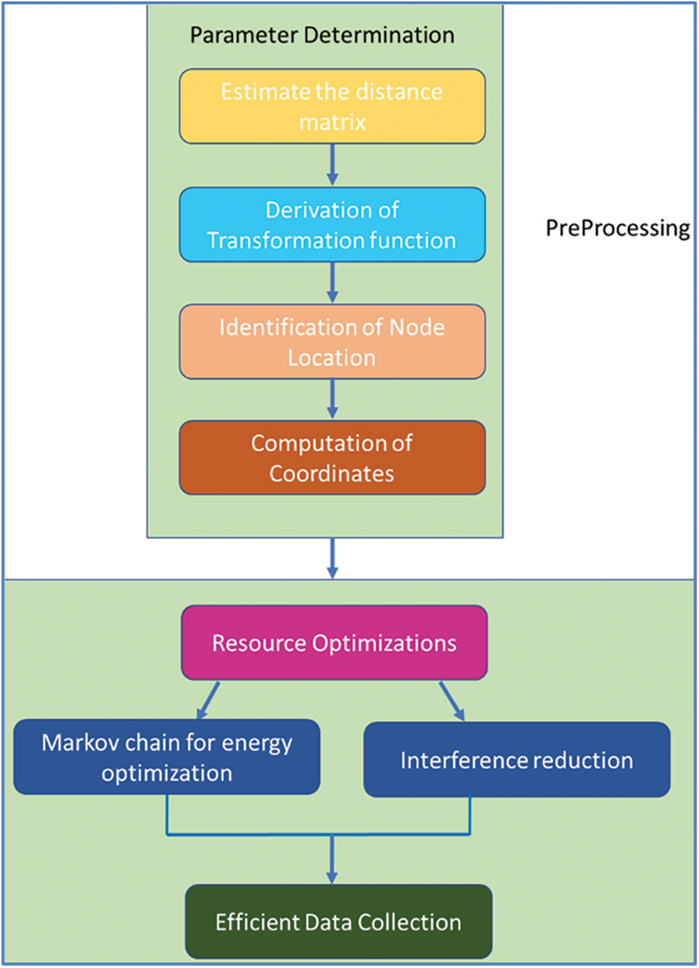
Figure 1: Architecture of proposed DM-MC method

4.1 Preprocessing

One of the essential operations in WSNs is system deployment. Consequently, to start the process, a list of empty nodes is initialized for each node. For a single anchor, the linked list is assigned with the distance of adjacent nodes, anchor ID, hop number and other location information. The distance detection between the nodes is carried out only after the nodes connect. The distance may then be calculated by combining the hop ranges between the nodes. All the nodes are assigned with the weight of 1. In large WSN, to reduce communication costs, a threshold is defined so that the distance cannot exceed the threshold value.

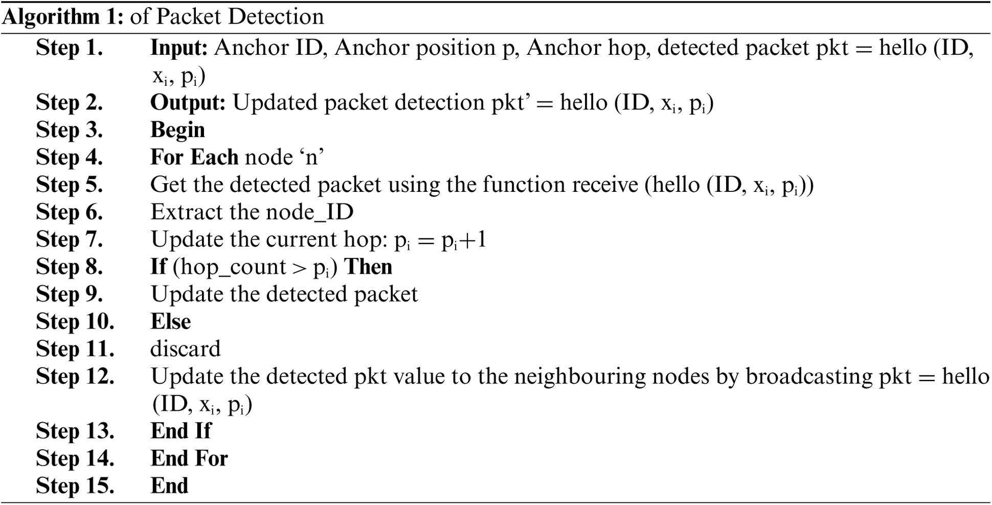
Each anchor node can then send a “Hello” message to its immediate neighbour nodes. The node continues the detection of packet process until the threshold value is reached. With the beginning value set to 0, the packet's content corresponds to the anchor node_ID, coordinate ‘xi’, and hop range ‘pi’. The hop range is incremented by one and is compared with the threshold whenever a non-anchor node receives a detection packet. If the hop range exceeds the threshold value set, then discard the packet. If not, it is advisable to retain the hop for future transmissions to maintain the node-link list up to current. The task is accomplished using the Algorithm 1 below.

4.2 Parameter Determination

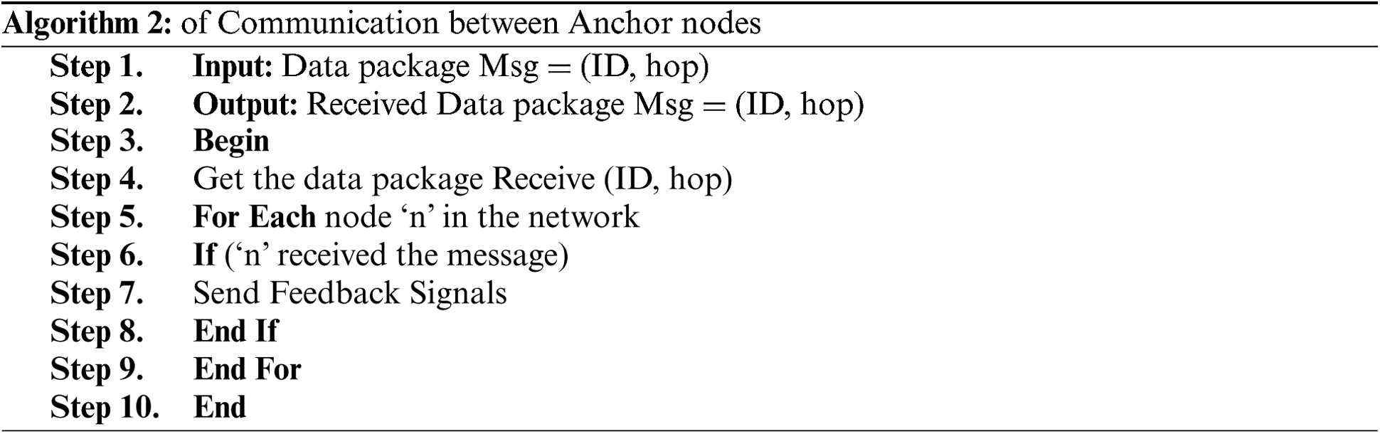
Each anchor node collects the updated information of the data package from another anchor node based on the preprocessing carried out. Algorithm 2 presented below describes the pseudo-code for anchor node communication. Once the above-discussed information is acquired, update the anchor node's connection list, notably the hop count.

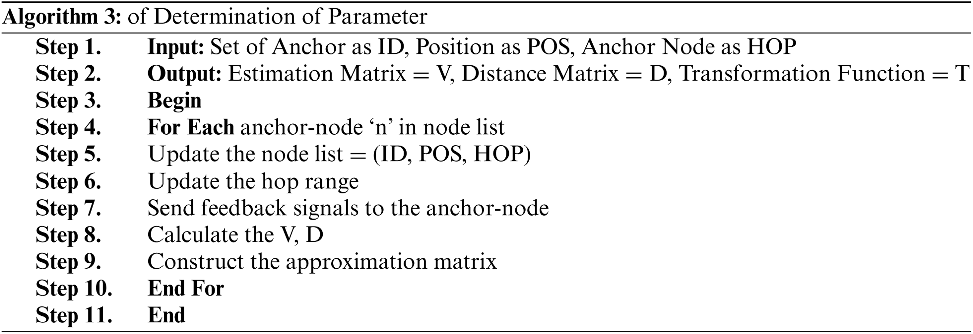
Then, in terms of the WSN, there is a straightforward method for constructing the estimate and distance matrices. If all of the anchor nodes update the key information, the closest nodes in the distance are picked to create a new approximate value matrix. At this period, the node localization variables are set. The method of selecting parameters may be explained using Algorithm 3.

4.3 Resource Optimization

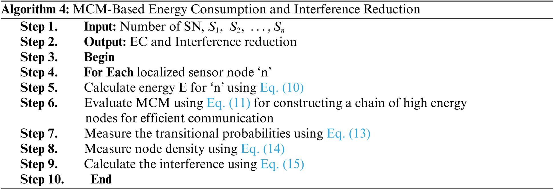
An energy measure is used to increase the data collecting efficiency in WSN, which is obtained via the MCM. Changes in the status of nodes are considered in the MCM. As a result, in order to increase the performance of WSN, a MCM is constructed for selecting higher energy SN.

In the suggested DM-MC technique, Fig. 2 illustrates MCM based resource optimizations to offer lower EC and effective interference reduction to increase data collection. A MCM is built to assess the equilibrium distribution by selecting greater energy and minimal drain rate nodes. The network's SN is processed using the MCM with a transitional model, and the energy of a sensor node is measured as illustrated below.

Energy(E)=Power(P)∗time(T)(14)

Energy (E) is defined as the product of power and time in Eq. (14). Unit of energy is Joule (J), the Watt (W) is the unit of power, and the unit of time is Second (S). A MCM is created with the measured energy, with the current state determining the system's future condition while past states are ignored. As a result, the sensor node's state change process is effectively monitored in the WSN. The following is a formula for constructing a MCM with a higher energy sensor node for efficient routing.

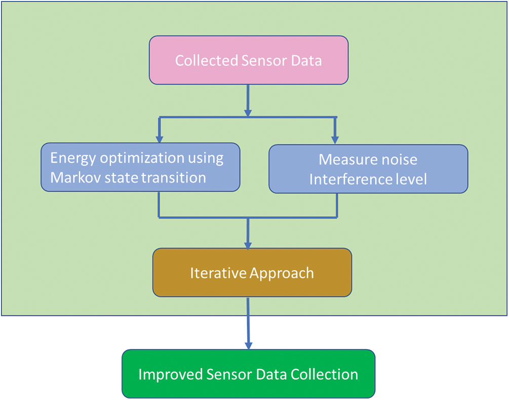
Figure 2: MCM based iterative resource optimizations technique

Markovchain=(Sq+1=s|s1=S1,s2=S2…sn=Sn)(15)

Sq+1 represents the next state of a sensor node in Eq. (15), and (S1,S2,…,Sn) represents the probable chain for varying numbers of SN. As a result, the SN with a high level of energy are clustered together. For effective data transmission, the equilibrium distribution function aids in identifying the high energy level SN in the relevant channel. With the help of nearby nodes, equilibrium distribution considers higher energy SN. Finally, higher energy nodes from dispersed SN form a MCM for efficient transmission. When N states are considered, the transmission probability property is achieved. Then, using the current time ‘x's and the following time ‘y’, the transition probability Pxy is calculated. The suggested DM-MC technique solely considers the current state ‘x's while calculating transition probability. The Markov chain's property is given below in Eq. (16).

∀x,y,Pxy∈[0,1](16)

With the aid of transitional probabilities, SN with lesser energy is removed using the MCM. In a WSN, transitional probability aids the identification of nodes with lower energy, allowing higher energy nodes to be selected to reduce the execution time. In the DM-MC technique, the transitional probability is as follows.

TransitionalProbability=∑nϵS⁡Pxk,Pyn−kk=0,1,2,…,n(17)

S indicates the state space transition in Eq. (17), and n denotes the number of SN in a network. The lowest energy SN is eliminated using the highest order transitional probability. As a result, energy usage is closely monitored in order to improve data transmission in WSN.

4.4 Noise Interference Reduction

After selecting higher energy nodes for data collection in a WSN, minimizing interference on the communication channel is considered. In order to accomplish effective routing in WSN, the proposed DM-MC approach aids in the selection of SN with better data transmission capabilities and low noise disturbance levels. Because of their unpredictable mobility in a network, interference occurs among distributed SN during data gathering, and its surroundings and transmission power cause a sensor node's interference. The Poisson distribution is used to measure the interference of WSNs, and the node density is calculated as shown below Eq. (18).

ρ=NA(18)

Sensor node density (ρ)is defined as the ratio of the total SN-N to the network area A in which the nodes are deployed. In a Poisson distribution, the interference area is denoted asAi. As a result, ρAiis used to calculate the number of SN placed in Ai. ρAiiis the same as Variance ‘σ’ in the distribution. The following mathematical construction produces randomly distributed SN.

NI=ρAi+3(ρAi)1/2(19)

Interference in a sensor node ‘NI’ is quantified using Eq. (19). These interferences are reduced by selecting SN with the highest transmission capabilities and the least noise disruption. As a result, the proposed DM-MC technique significantly enhances sensor node communication. Algorithm 4 shows the stages for MCM-based EC and interference reduction.

Energy optimization is done by constructing a MCM with higher energy localized SN. Furthermore, the node communication channel is supplied with little interference by selecting a greater data transmission capability and a low noise disturbance level. To better data gathering, interference is assessed in terms of node density and network area.

5  Experimental Evaluation

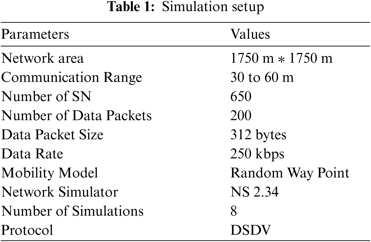
Network Simulator-2 is used to test the proposed DM-MC technique. In the WSN, 650 SN is distributed at random over a 1750 m × 1750 m region. The number of SN in the network where node localization and interference reduction are conducted is called node density. The simulation settings and their values are shown in Tab. 1.

The proposed DM-MC method is analysed with the metrics such as node location identification accuracy, execution time, EC and interference reduction rate.

5.1 Results and Discussion

The proposed DM-MC method is compared to existing methods given by Bianchi et al. 2020 [29,30] and Mubaraka's CSA model presented in Kaur et al. 2019 [31].

5.2 Impact of Node Location Identification Accuracy

The number of SN localised by identifying their positions to the total number of SN in a WSN is known as node location identification accuracy. The following formula is used to calculate the accuracy of sensor node position identification [32–35].

NLIA=localizedsensornodesnumberofsensornodes∗100(20)

The percentage (%) of Node Location Identification Accuracy (NLIA) is calculated using Eq. (20). A method's performance is enhanced by higher sensor node location identification accuracy.

The accuracy of node location identification using the DM-MC technique and other current methods is tabulated in Tab. 2. To measure, 10 simulations with varying number of SN (50 to 650) are run. Tab. 2 shows that increasing the number of SN improves node location recognition accuracy for all techniques. However, compared to current techniques, the suggested DM-MC method achieves the highest node location identification accuracy.

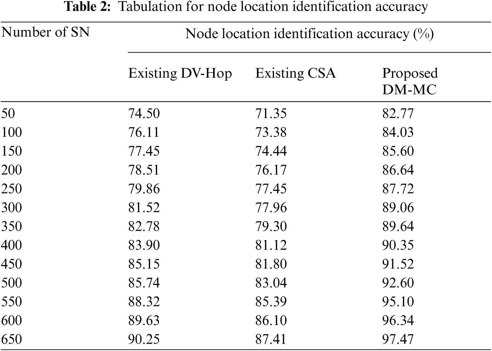
Fig. 3 compares the proposed DM-MC approach to existing DV-Hop and existing CSA in node location identification accuracy Vs the number of SN. Fig. 3 shows how the suggested DM-MC technique uses Distance Matrix and Markov Chain to increase node position recognition accuracy. A target node determines its location based on the positions of its neighbours and coordinates the information from surrounding SN, and sensor Node local and global convergence aid in determining sensor node position. Consequently, the suggested DM-MC approach improves node location identification accuracy by 9% compared to the current DV-Hop method and 13% compared to the existing CSA method [36–39].

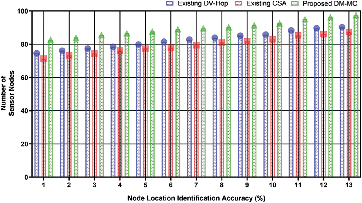
Figure 3: Measure of node location identification accuracy

5.3 Impact of Execution Time

The time taken by SN in a WSN to determine their positions is used to calculate the execution time for node localization. The execution time is calculated as a function of the number of SN (n). The following is the mathematical formula for calculating execution time.

ET=n∗Time(identifysensornodelocation)(21)

The Execution Time ‘ET’ in milliseconds (ms) may be calculated using Eq. (21). If a technique is more efficient, the execution time for node localization is reduced.

Tab. 3 shows the execution time for the recommended DM-MC, existing DV-Hop, and CSA node localization approaches as a function of the number of SN. Between 50 and 650, the SN is expected to be present. Tab. 3 shows that the execution time for node localization rises as the number of SN grows for all approaches. The proposed DM-MC technique effectively decreases the execution time for node localization when compared to prior methodologies.

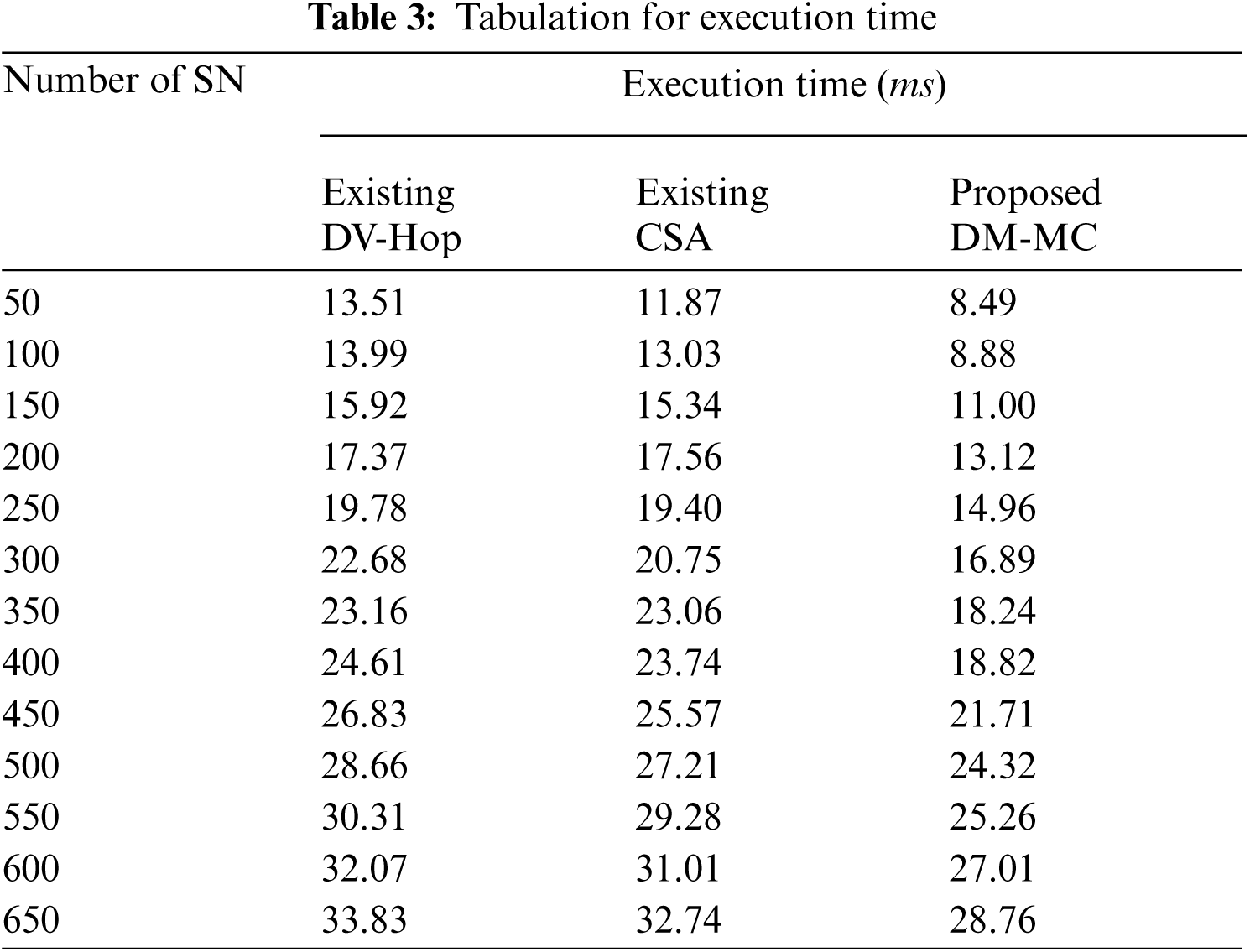
Fig. 4 shows the execution time for node localization in WSN utilizing the proposed DM-MC technique compared to current methods as DV-Hop and CSA. Using a Hyperbolic-based Least Square Estimation model, the suggested DM-MC technique considerably decreases the execution time compared to other methods. With the aid of a linear relationship, a least-square estimate is accomplished based on the acquired local and global convergence of SN. In order to get a specific node ID, the distance between focus points and the source node is measured using a linear equation form. When all SN in a WSN converge, the execution time is reduced by 33% compared to the existing DV-Hop technique and 27% compared to the existing CSA approach, respectively.

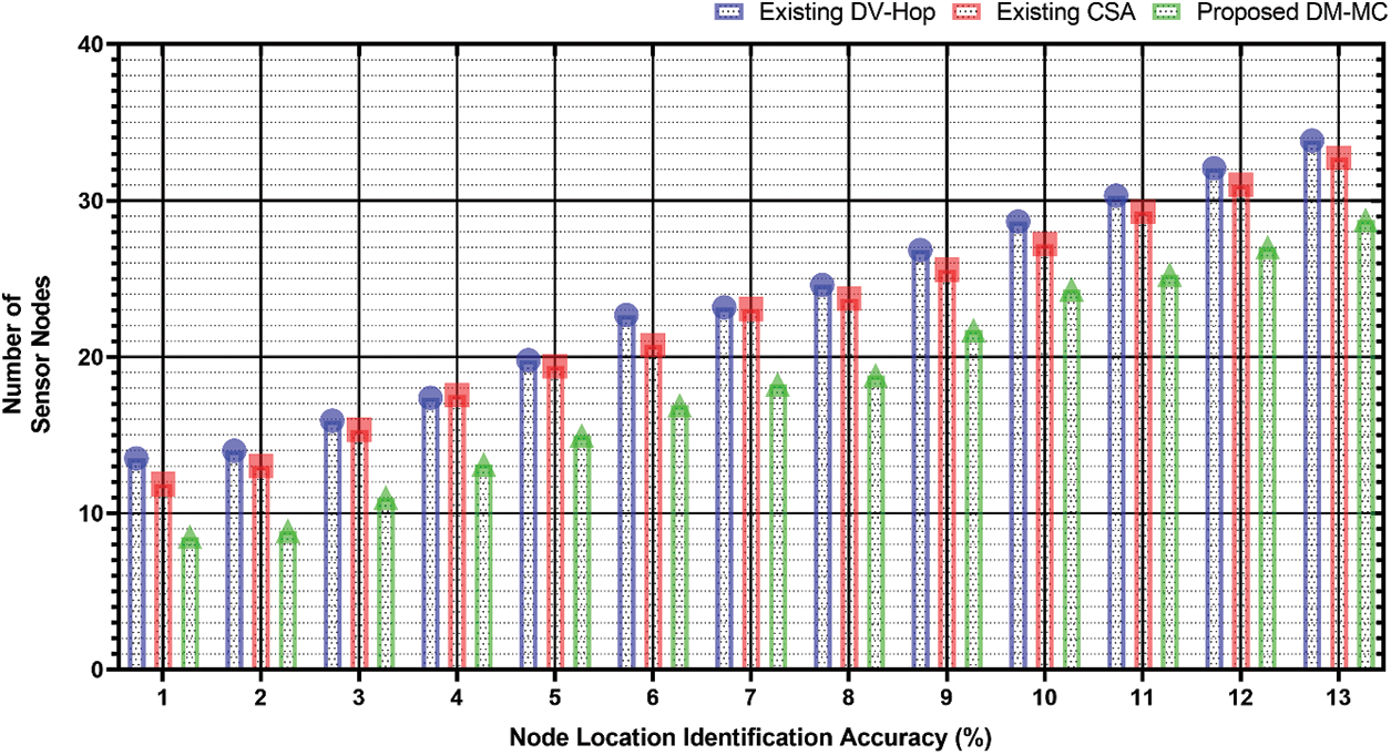
Figure 4: Measure of execution time

5.4 Impact of Energy Consumption

The number of high energy SN and the energy used by a single sensor node to reach the sink node are used to calculate EC among SN in a WSN. Below is a mathematical representation of energy usage.

EC=numberofhighenergysensornodes∗ECs(22)

Energy Consumption ‘EC’ is calculated using Eq. (22), depending on the energy consumed by a single sensor node ‘ECs’ in a Markov chain, and the number of high-energy SN. Joules are the units of measurement for EC. In WSN, providing low EC increases a method's performance.

The EC of the proposed DM-MC technique and other current methods is shown in Tab. 4. For conducting tests, the number of SN is changed from 50 to 650. For all methods in Tab. 4, energy usage increases as the number of SN increases. Though compared to other current approaches, the suggested DM-MC method successfully decreases EC in WSN.

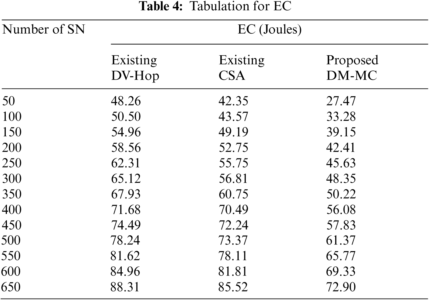
Fig. 5 depicts the proposed DM-MC approach, the existing DV-Hop, and CSA models. As demonstrated in Fig. 5, the proposed DM-MC methodology utilizes less energy than previous methods by employing the MCM. The next state of a node in a Markov Chain is decided only by its present state. As a result of the state transition, lower energy SN is eliminated, and higher energy SN is picked. Transition probability is used in the Markova chain to sustain higher energy nodes. Finally, the proposed DM-MC approach decreases energy use by 31% and 25%, respectively, compared to the existing DV-Hop and CSA methods.

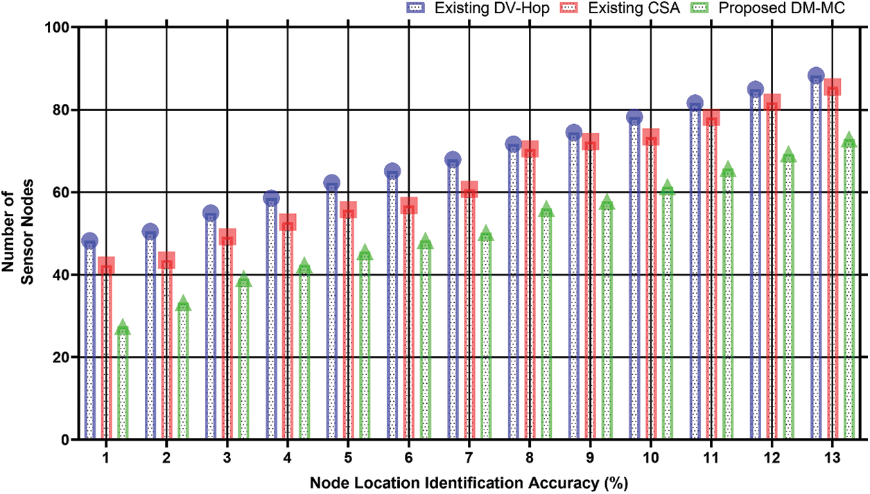
Figure 5: Measure of EC

6  Conclusion

The proposed localization model “DM-MC” concentrates on identifying the position of the SN in the WSNs. The node is accurately identified using distance matrix and Markov chain optimization techniques. This model generates a more dependable output by identifying the exact location of a sensor node. System scalability is ensured through this model by incorporating the MCM. The experimental results were performed against two proven models, DV-Hop and CSA algorithms, showing that the proposed DM-MC model outperforms both the existing models regarding localization accuracy and EC. These results add to the credibility of the proposed model as a better model for employing node localization while establishing a WSN framework.

Funding Statement: This project was funded by the Deanship of Scientific Research (DSR) at King Abdulaziz University, Jeddah, under Grant No. (RG-91-611-42). The authors, therefore, acknowledge with thanks to DSR technical and financial support.

Conflicts of Interest: The authors declare that they have no conflicts of interest to report regarding the present study.

This work is licensed under a Creative Commons Attribution 4.0 International License, which permits unrestricted use, distribution, and reproduction in any medium, provided the original work is properly cited.