DOI:10.32604/cmc.2022.023683
| Computers, Materials & Continua DOI:10.32604/cmc.2022.023683 | |
| Article |
Prediction of Changed Faces with HSCNN
Department of Liberal Studies (Computer), Korean Bible University, Seoul, 01757, Korea
*Corresponding Author: Jinho Han. Email: hjinob@bible.ac.kr
Received: 17 September 2021; Accepted: 19 October 2021
Abstract: Convolutional Neural Networks (CNN) have been successfully employed in the field of image classification. However, CNN trained using images from several years ago may be unable to identify how such images have changed over time. Cross-age face recognition is, therefore, a substantial challenge. Several efforts have been made to resolve facial changes over time utilizing recurrent neural networks (RNN) with CNN. The structure of RNN contains hidden contextual information in a hidden state to transfer a state in the previous step to the next step. This paper proposes a novel model called Hidden State-CNN (HSCNN). This adds to CNN a convolution layer of the hidden state saved as a parameter in the previous step and requires no more computing resources than CNN. The previous CNN-RNN models perform CNN and RNN, separately and then merge the results. Therefore, their systems consume twice the memory resources and CPU time, compared with the HSCNN system, which works the same as CNN only. HSCNN consists of 3 types of models. All models load hidden state ht−1 from parameters of the previous step and save ht as a parameter for the next step. In addition, model-B adds ht−1 to x, which is the previous output. The summation of ht−1 and x is multiplied by weight W. In model-C the convolution layer has two weights: W1 and W2. Training HSCNN with faces of the previous step is for testing faces of the next step in the experiment. That is, HSCNN trained with past facial data is then used to verify future data. It has been found to exhibit 10 percent greater accuracy than traditional CNN with a celeb face database.
Keywords: CNN-RNN; HSCNN; hidden state; changing faces
Face recognition (FR) systems have been continually developed for personal authentication. These efforts have resulted in FR applications acting on mobile phones [1]. Researchers have proposed several ideas for FR systems: eigen faces [2], independent component analysis [3], linear discriminant analysis [4,5], three-dimensional (3D) method [6–9], and liveness detection schemes to prevent the misuse of photographic images [10]. Using data acquisition methodology, Jafri et al. [11] divided FR techniques into three categories: intensity images, video sequences, and 3D or infra-red techniques. They introduced AI approaches as one of the operating methods for intensity images and reported that it worked efficiently for somewhat complex FR scenarios. Such techniques had not previously been utilized for practical everyday purposes.
In 2012, AlexNet [12] was proposed and became a turning point in large-scale image recognition. It was the first CNN, one of the deep learning techniques, and was declared the winner of the ImageNet Large Scale Visual Recognition Challenge (ILSVRC) 2012 with 83.6% accuracy. In ILSVRC 2013, Clarifai was the winner with 88.3% [13,14], whereas in ILSVRC 2014, GoogLeNet was the winner with 93.3% [15]. The latter was an astonishing result because humans trained for annotator comparison exhibited approximately 95% accuracy in ILSVRC [16]. In 2014, using a nine-layer CNN, DeepFace [17] achieved 97.35% accuracy in FR, closely approaching the 97.53% ability of humans to recognize cropped Labeled Faces in the Wild (LFW) benchmark [18]. However, DeepID2 [19] achieved 99.15% face verification accuracy with the balanced identification and verification features on ConvNet, which contained four convolution layers. In 2015, DeepID3 [20] achieved 99.53% accuracy using VGGNet (Visual Geometry Group Net) [21], whereas FaceNet [22] achieved 99.63% using only 128-bytes per face.
CNN consists of convolution layers, pooling layers, and fully connected layers. However, a number of problems still needed to be addressed. For instance, CNN trained with past images failed to verify changed images according to a time sequence. In their in-depth FR survey, Wang et al. [23] described three types of cross-factor FR algorithms as challenges to address in real-world applications: cross-pose, cross-age, and makeup. Cross-age FR is a substantial challenge with respect to facial aging over time. Several researchers have attempted to resolve this issue. For instance, Liu et al. [24] proposed an age estimation system for faces with CNN. Bianco et al. [25] and Khiyari et al. [26] applied CNN to learn cross-age information. Li et al. [27] suggested metric learning in a deep CNN. Other studies have suggested combining CNN with recurrent neural networks (RNN) to verify changed images because RNN can predict data sequences [28]. RNN contains contextual information in a hidden state to transfer a state in the previous step to the next step, and has been found to generate sequences in various domains, including text [29], motion capture data [30], and music [31,32].
This paper proposes a novel model called Hidden State-CNN (HSCNN) as well as training the modified CNN with past data to verify future data. HSCNN adds to CNN a convolution layer of the hidden state saved as a parameter. The contributions of the present study are as follows:
First, the proposed model, HSCNN, exhibits 10 percent greater accuracy than traditional CNN with a celeb face database [33]. Facial images of the future were tested after training based on facial images of the past. HSCNN adds the hidden state saved as a parameter in the previous step to the CNN structure. Further details on this process are provided in Section 4.2.
Secondly, because HSCNN included the hidden state of RNN in the proposed architecture, it was efficient in its use of computing resources. Other researchers have performed CNN and RNN, separately, and merged the results in the system, consuming double the number of resources and processing time. Further details are presented in Section 2.
Thirdly, this paper indicates that HSCNN can train with only two images of one person per step. Also, the loss value reached 0.4 in just 40 epochs in training with loading parameters and 250 epochs in training without loading parameters. Therefore, the HSCNN achieves efficiency because it uses only two images and trains in 40 epochs with loading parameters. This is explained further in Section 4.1.
In the remainder of this paper, Section 2 introduces related works, Section 3 outlines the proposed method, Section 4 presents the experimental results, and Section 5 provides the conclusion.
Some neural network models can acquire contextual information in various text environments using recurrent layers. Convolutional Recurrent Neural Networks (CRNN) works for a scene text recognition system to read scene texts in the image [34]. It contains both convolutional and LSTM recurrent layers of the network architecture and uses past state and current input to predict the subsequent text. Recurrent Convolutional Neural Networks (RCNN) also uses a recurrent structure to classify text from document datasets [35]. The combined CNN and RNN model uses relations between phrases and word sequences [36] and in the field of natural language processing (NLP) [37].
Regarding changed images, combining CNN with RNN methods have been proposed in image classification [38] and a medical paper for blood cell images [39]. These authors merged the features extracted from CNN and RNN to determine the long-term dependency and continuity relationship. A CNN-LSTM algorithm was proposed for stock price prediction according to leading indicators [40]. This algorithm employed a sequence array of historical data as the input image of the CNN and feature vectors extracted from the CNN as the input vector of LSTM. However, these methods used CNN and RNN, separately, and merged the results vectors extracted from CNN to RNN. Therefore, their systems consume twice the memory resources and CPU time, compared with the proposed system, which works the same as CNN only. Fig. 1 presents an overview of the models developed by Yin et al. [38] and Liang et al. [39].
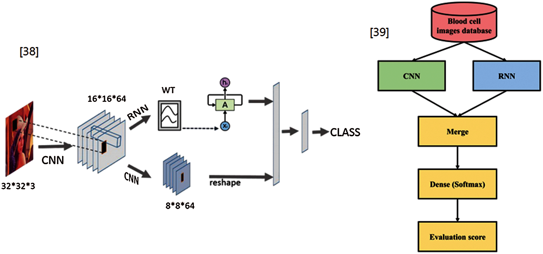
Figure 1: Overview of previous CNN-RNN models
Han introduced incremental learning in CNN [41]. Incremental-CNN (I-CNN) was tested using the MNIST dataset. HSCNN referenced I-CNN, which used hidden states (ht−1, ht) and an added convolution layer. For training, I-CNN used the MNIST database of handwritten digits comprising 60,000 examples and changed handwritten digits (CHD) comprising 1,000 images. This paper proposes HSCNN, a new structure combining CNN with RNN. It adds a hidden state of RNN into a convolution layer of CNN. Consequently, HSCNN acts like CNN and performs efficiently for cross-age FR.
3 Proposed Method: Hidden State CNN
The following subsections explain the equation of the loss function cross-entropy error and optimizer of the stochastic gradient descent used in the proposed method. And then, 3 types of models of Hidden State CNN are described.
3.1 Loss Function and Optimizer
In HSCNN, experiments indicated that cross-entropy error (CEE) was the appropriate loss function (cost function or objective function). The best model has a cross-entropy error of 0. The smaller the CEE, the better the model. The CEE equation is:
where tk is the truth label, and yk is the softmax probability for the kth class. When calculating the log, a minimal value near the 0.0 delta is necessary to prevent a ‘0’ error. In the python code, the CEE equation is:
Also, the optimizer is the stochastic gradient descent (SGD), which is a method for optimizing a loss function. The equation is:
where W is the weight,
HSCNN consists of 3 types of models: model-A, model-B, and model-C. Model-A is the same as I-CNN. Fig. 2 presents the overall structure of HSCNN, which is the modified AlexNet with hidden state ht of Convolution layer 5. HSCNN consists of convolution layers, RelU function, pooling layers, affine layers, and soft max function such as traditional CNN, but it also has hidden states: ht−1 and ht. This distinguishes HSCNN from CNN.
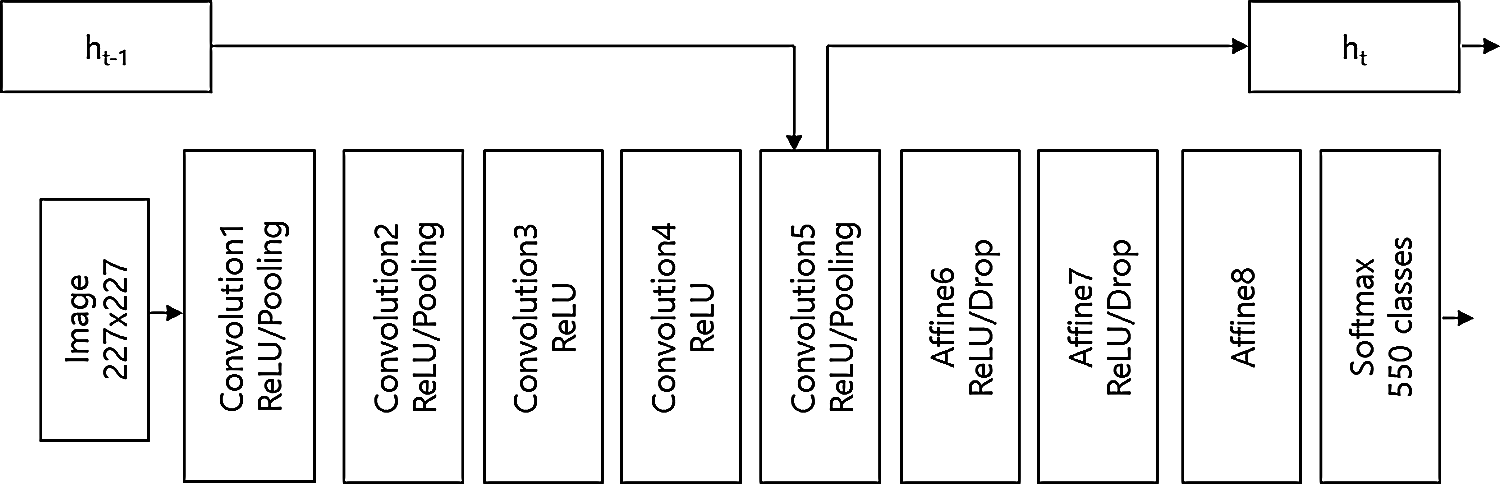
Figure 2: The overall structure of HSCNN
Fig. 3 presents the structure of model-A. Model-A loads hidden state ht−1 from the parameters of the previous step and saves ht as a parameter for the next step. It adds the convolution layer 6 and W2. The activation function of the rectified linear unit (RelU) equation of model-A is:
Fig. 4 presents the structure of model-B. Model-B loads hidden state ht−1 from parameters of the previous step and saves ht as a parameter for the next step. The model adds ht−1 to x, which was the previous output. The summation of ht−1 and x is multiplied by weight W. The activation function of the rectified linear unit (RelU) equation of model-B is:
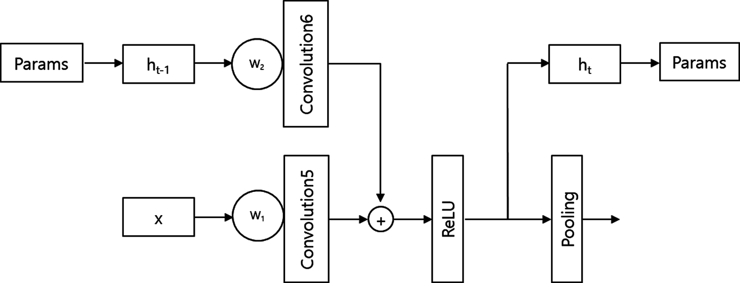
Figure 3: The structure of model-A of HSCNN

Figure 4: The structure of model-B of HSCNN
Fig. 5 presents the structure of model-C. Model-C loads hidden state ht−1 from parameters of the previous step and saves ht as av parameter for the next step. In this case, the convolution layer has two weights: W1 and W2. The activation function of the rectified linear unit (RelU) equation of model-C is:

Figure 5: The structure of model-C of HSCNN
In the experiment, HSCNN used Cross-Entropy Error as the loss function, Stochastic Gradient Descent (SGD) as the optimizer, and the Instruction rate (Ir) was 0.001. HSCNN also used python, NumPy library, and CuPy library for the NVIDIA GPUs employed for software coding.
4.1 Preparations for Experiments
The essential items required for the experiments are listed in Tab. 1. The experiments used FaceApp Pro to make old faces from young faces and Abrosoft Fanta Morph Deluxe to generate 100 morphing facial images between young and old faces.
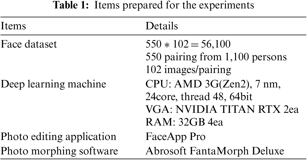
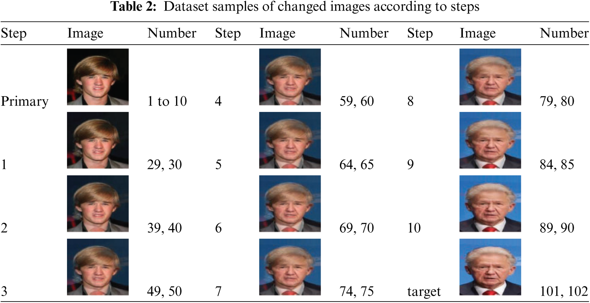
The facial images of 1,100 persons were selected from the celeb face database, known as the Large-scale CelebFaces Attributes (CelebA) Dataset. Those faces were then paired with a similar face; for example, man to man, woman to woman, Asian to Asian, and so on. One was chosen as the young face between paired faces and the other was changed to the old face. To make these changes, the photo editing application FaceApp Pro was used. Between the transition from young faces to old faces, 100 continually changing faces were created using the photo morphing software FantaMorph.
The difference between the young and old images of the same person made by FaceApp Pro was not sufficient, so the experiments also paired the faces of two other persons. Thus, the young face and old face of each pair were different persons. Finally, 102 images changing from young to old were created for all 550 paired images. Number 1 is the youngest image, and number 102 is the oldest. 102 images show the aging state over time from young to old. Number 1 is the youngest image, and number 102 is the oldest. 102 images show the aging state over time from young to old. Numbers 1 to 10 are young images used as the first training data, and the last numbers 101 to 102 are old images and used as final target images. Using 90 images from numbers 11 to 100, the experiments used 10 steps to learn and test aging changes over time. When learning using 9 images in each of 10 steps, all 90 images are used. However, in this case, learning occurs on the entire data, and the training result of the proposed model or CNN was almost the same. So the prediction experiments become meaningless. Therefore, to clearly confirm the results of the prediction experiment, two images are trained for each step, and the two images mean a specific point in the middle of facial aging. This is the same as testing the face at the last oldest point with two final target images. Tab. 2 presents sample images from the dataset and their numbers for each step: primary step, target step, and step 1 to step 10. Beyond primary step, each step has only two samples. There is a substantial difference between images number 60 to number 90; however, after number 90, all facial images look almost identical.
HSCNN appears to be an extremely efficient method as it achieved 99.9% accuracy and 0.01 loss value with only two training images in each step from step 1 to step 10. Also, the HSCNN is trained with loading parameters saved in the previous step. The use of loading parameters means the training epochs can be shortened. Fig. 6 indicates that the loss value reaches 0.4 in 250 epochs in training without loading parameters and just 40 epochs with loading parameters. Thus, the HSCNN achieves efficiency because it uses only two images and trains in 40 epochs with loading parameters.

Figure 6: The efficiency of HSCNN
The experiments utilized AlexNet as the traditional CNN and created three models of HSCNN modifying AlexNet. All models added hidden states to the convolution five-layer and used the RelU 5 layer of the AlexNet.
Fig. 7 presents the samples of train steps of the experiments and it shows the accuracy of each training step and loss values through 150 epochs. In the case of training step 3 of model-A, the graph shows the accuracy of training step 3, testing of step 4, step 5, step 6, step 7, step 8, step 9, step 10, and target step. It also shows the loss values according to the epochs. For including loss values in one graph, loss values were divided by 10.

Figure 7: The samples of train steps of the experiments
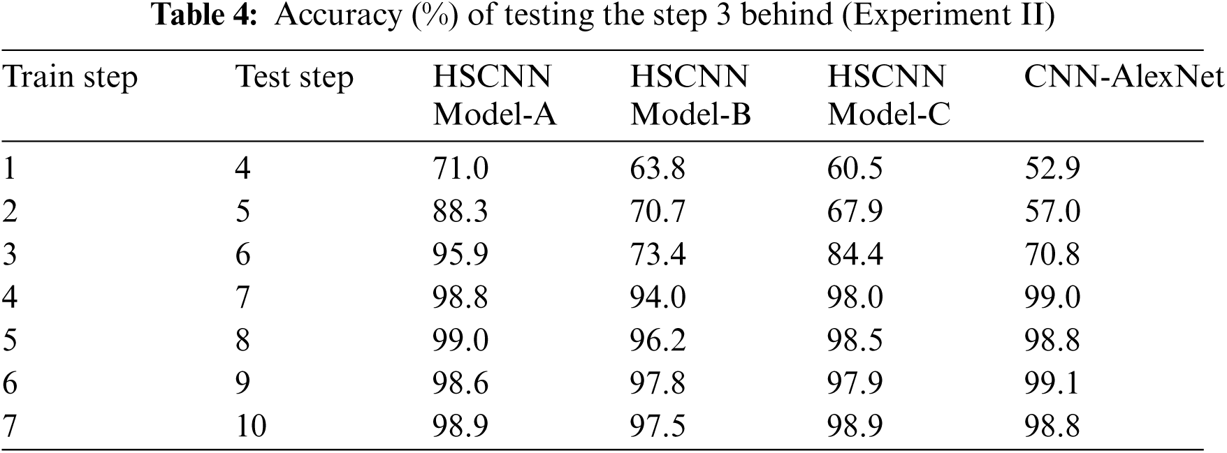
The experiments consisted of 2 groups: experiment I, experiment II. Experiment I tested the target step, and experiment II tested step 3 (behind the training step). Step 1 employed the parameters saved in the primary step, while step 2 used the parameters saved in step 1.
Tab. 3 presents the accuracy of the target step in testing faces. Tab. 4 presents the accuracy of step 3 behind, according to the models, in testing faces. The test of step 3 behind means that HSCNN tested step 4 when training step 1, and step 5 when training step 2.
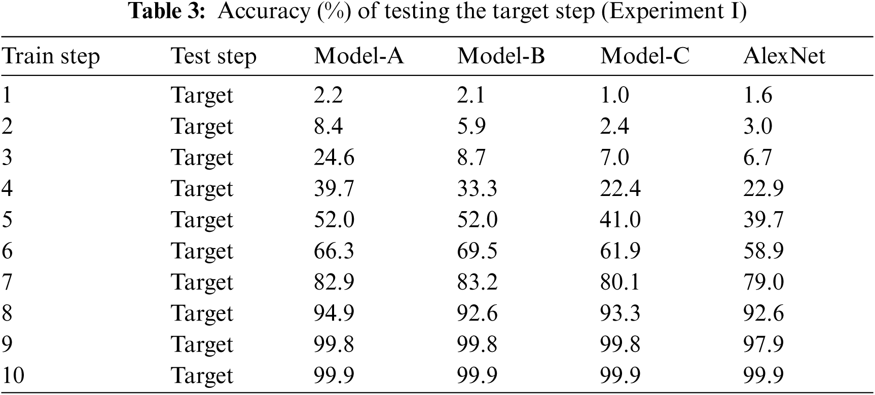
Based on Tabs. 3 and 4, the results of the experiments are presented in Figs. 8–10. Fig. 8 depicts the differences between model-A and AlexNet. These indicate that model-A achieved more than 10% higher accuracy in step 3 to step 5 of experiment I and in step 1 to step 3 of experiment II. Therefore, model-A can be employed for both long- and short-time changes.

Figure 8: The results of the model-A and AlexNet experiments

Figure 9: The results of model-B and AlexNet experiments

Figure 10: The results of model-C and AlexNet experiments
Fig. 9 depicts the differences between model-B and AlexNet. These indicate that model-B achieved more than 10% higher accuracy in step 4 to step 6 of experiment I and in step 1 to step 2 of experiment II. Therefore, model-B can be employed to predict both long- and short-time changes. Fig. 10 depicts the differences between model-C and AlexNet. These indicate that model-C achieved more than 10% higher accuracy in step 2 to step 3 of experiment II, but not in any step of experiment I. Therefore, model-C is considered an appropriate method to predict short-time changes.
This paper proposes a novel model, Hidden State-CNN (HSCNN), which adds to CNN a convolution layer of the hidden state. Training with past data to verify future data was the aim of the experiments, and HSCNN exhibited 10 percent higher accuracy with the celeb face database than the traditional CNN. The experiments consisted of 2 groups. Experiment I tested the target step and experiment II tested step 3 behind the training step. The latter step means that step 4 was tested when training step 1. Experiment I assessed long-time changes, and experiment II relatively short-time changes. Both yielded similar results. Furthermore, HSCNN achieved a more efficient use of computing resources because its structure differed from that of other CNN-RNN methods. HSCNN also represented a new and efficient training process to verify changing faces. It used only two training images in each step and achieved 99.9% accuracy and 0.01 loss value.
Funding Statement: This work was supported by the National Research Foundation of Korea (NRF) grant in 2019 (NRF-2019R1G1A1004773).
Conflicts of Interest: The author declares that he has no conflicts of interest to report regarding the present study.
1. C. Bhagavatula, B. Ur, K. Iacovino, S. M. Kywe, L. F. Cranor et al., “Biometric authentication on iPhone and android: usability, perceptions, and influences on adoption,” in Proc. USEC ‘15: Workshop on Usable Security, San Diego, CA, USA, pp. 1–10, 2015. [Google Scholar]
2. M. Turk and A. Pentland, “Eigenfaces for recognition,” Journal of Cognitive Neuroscience, vol. 3, no. 1, pp. 71–86, 1991. [Google Scholar]
3. M. S. Bartlett, J. R. Movellan and T. J. Sejnowski, “Face recognition by independent component analysis,” IEEE Transactions on Neural Networks, vol. 13, no. 6, pp. 1450–1464, 2002. [Google Scholar]
4. P. Belhumeur, J. Hespanha and D. Kriegman, “Eigenfaces vs. fisherfaces: recognition using class specific linear projection,” in Proc. of the Fourth European Conf. on Computer Vision, vol. 1, Cambridge, UK, pp. 45–58, 1996. [Google Scholar]
5. L. Juwei, K. N. Plataniotis and A. N. Venetsanopoulos, “Face recognition using LDA-based algorithms,” IEEE Transactions on Neural Networks, vol. 14, no. 1, pp. 195–200, 2003. [Google Scholar]
6. K. W. Bowyer, K. Chang and P. Flynn, “A survey of approaches and challenges in 3d and multi-modal 3d+ 2d face recognition,” Computer Vision and Image Understanding, vol. 101, no. 1, pp. 1–15, 2006. [Google Scholar]
7. A. Scheenstra, A. Ruifrok and R. C. Veltkamp, “A survey of 3d face recognition methods,” in Proc. Int. Conf. on Audio- and Videobased Biometric Person Authentication, vol. 3546, pp. 891–899, 2005. [Google Scholar]
8. A. F. Abate, M. Nappi, D. Riccio and G. Sabatino, “2d and 3d face recognition: A survey,” Pattern Recognition Letters, vol. 28, no. 14, pp. 1885–1906, 2007. [Google Scholar]
9. L. Ballihi, B. B. Amor, M. Daoudi, A. Srivastava and D. Aboutajdine, “Boosting 3-d-geometric features for efficient face recognition and gender classification,” IEEE Transactions on Information Forensics and Security, vol. 7, no. 6, pp. 1766–1779, 2012. [Google Scholar]
10. H. K. Jee, S. U. Jung and J. H. Yoo, “Liveness detection for embedded face recognition system,” International Journal of Biomedical Sciences, vol. 1, no. 4, pp. 235–238, 2006. [Google Scholar]
11. R. Jafri and H. R. Arabnia, “A survey of face recognition techniques,” Journal of Information Processing Systems, vol. 5, no. 2, pp. 41–68, 2009. [Google Scholar]
12. A. Krizhevsky, I. Sutskever and G. E. Hinton, “Imagenet classification with deep convolutional neural networks,” Neural Information Processing Systems, vol. 1, pp. 1097–1105, 2012. [Google Scholar]
13. M. D. Zeiler and R. Fergus, “Visualizing and understanding convolutional networks,” in European Conf. on Computer Vision of Lecture Notes in Computer Science, Zurich, Switzerland, Springer, vol. 8689 pp. 818–833, 2014. [Google Scholar]
14. M. D. Zeiler, G. W. Taylor and R. Fergus, “Adaptive deconvolutional networks for mid and high level feature learning,” in Int. Conf. on Computer Vision, Barcelona, Spain, pp. 2018–2025, 2011. [Google Scholar]
15. C. Szegedy, W. Liu, Y. Jia, P. Sermanet, S. Reed et al., “Going deeper with convolutions,” ArXiv:1409.4842, 2014. [Google Scholar]
16. O. Russakovsky, J. Deng, H. Su, J. Krause, S. Satheesh et al., “Imagenet large scale visual recognition challenge,” International Journal of Computer Vision, vol. 115, no. 3, pp. 211–252, 2015. [Google Scholar]
17. Y. Taigman, M. Yang, M. Ranzato and L. Wolf, “Deepface: Closing the gap to human-level performance in face verification,” in IEEE Conf. on Computer Vision and Pattern Recognition, Columbus, OH, USA, pp. 1701–1708, 2014. [Google Scholar]
18. G. B. Huang, M. Ramesh, T. Berg and E. Learned-Miller, “Labeled faces in the wild: A database for studying face recognition in unconstrained environments,” In Technical Report, University of Massachusetts, Amherst, HAL-Inria, pp. 07–49, 2007. [Google Scholar]
19. Y. Sun, Y. Chen, X. Wang and X. Tang, “Deep learning face representation by joint identification-verification,” in Proc. of the 27th Int. Conf. on Neural Information Processing Systems, Montreal Canada, vol. 2, pp. 1988–1996, 2014. [Google Scholar]
20. Y. Sun, D. Liang, X. Wang and X. Tang, “Deepid3: Face recognition with very deep neural networks,” e-Print archive, ArXiv Preprint, arXiv:1502.00873, 2015. [Google Scholar]
21. K. Simonyan and A. Zisserman, “Very deep convolutional networks for large-scale image recognition,” ArXiv Preprint, arXiv:1409.1556, 2014. [Google Scholar]
22. F. Schroff, D. Kalenichenko and J. Philbin, “Facenet: A unified embedding for face recognition and clustering,” in Proc. IEEE Conf. on Computer Vision and Pattern Recognition, Boston, Massachusetts, pp. 815–823, 2015. [Google Scholar]
23. M. Wang and W. Deng, “Deep face recognition: A survey,” Neurocomputing, vol. 429, pp. 215–244, 2021. [Google Scholar]
24. X. Liu, Y. Zou, H. Kuang and X. Ma, “Face image Age estimation based on data augmentation and lightweight convolutional neural network,” Symmetry, vol. 12, no. 1, pp. 146–162, 2020. [Google Scholar]
25. S. Bianco, “Large age-gap face verification by feature injection in deep networks,” Pattern Recognition Letters, vol. 90, pp. 36–42, 2017. [Google Scholar]
26. H. E. Khiyari and H. Wechsler, “Age invariant face recognition using convolutional neural networks and set distances,” Journal of Information Security, vol. 8, no. 03, p. 174–186, 2017. [Google Scholar]
27. Y. Li, G. Wang, L. Nie, Q. Wang and W. Tan, “Distance metric optimization driven convolutional neural network for age invariant face recognition,” Pattern Recognition, vol. 75, pp. 51–62, 2018. [Google Scholar]
28. A. Graves, “Generating sequences with recurrent neural networks,” ArXiv Preprint, arXiv:1308.0850, 2013. [Google Scholar]
29. I. Sutskever, J. Martens, and G. Hinton, “Generating text with recurrent neural networks,” in Proc. Int. Conf. on Machine Learning, Bellevue, Washington, USA, 2011. [Google Scholar]
30. I. Sutskever, G. E. Hinton and G. W. Taylor, “The recurrent temporal restricted boltzmann machine,” International Conference on Neural Information Processing Systems, vol. 21, pp. 1601–1608, 2008. [Google Scholar]
31. N. Boulanger-Lewandowski, Y. Bengio and P. Vincent, “Modeling temporal dependencies in high-dimensional sequences: Application to polyphonic music generation and transcription,” in Proc. the Twenty-Nine Int. Conf. on Machine Learning (ICML’12Edinburgh, Scotland, UK, pp. 1159–1166, 2012. [Google Scholar]
32. D. Eck and J. Schmidhuber, “A first look at music composition using lstm recurrent neural networks,” Istituto Dalle Molle Di Studi Sull Intelligenza Artificiale, vol. 103, pp. 1–11, 2002. [Google Scholar]
33. S. Yang, P. Luo, C. C. Loy and X. Tang, “From facial parts responses to face detection: A deep learning approach,” in Proc. IEEE Int. Conf. on Computer Vision (ICCVSantiago, Chile, pp. 3676–3684, 2015, http://mmlab.i.e.,cuhk.edu.hk/projects/CelebA.html. [Google Scholar]
34. B. Shi, X. Bai and C. Yao, “An end-to-end trainable neural network for image-based sequence recognition and its application to scene text recognition,” IEEE Transactions on Pattern Analysis and Machine Intelligence, vol. 39, no. 11, pp. 2298–2304, 2017. [Google Scholar]
35. S. Lai, L. Xu, K. Liu and J. Zhao, “Recurrent convolutional neural networks for text classification,” in Proc. AAAI Conf. on Artificial Intelligence, Austin, Texas, USA, pp. 2267–2273, 2015. [Google Scholar]
36. S. T. Hsu, C. Moon, P. Jones and N. F. Samatova, “A hybrid CNN-rNN alignment model for phrase-aware sentence classification,” in Proc. the 15th Conf. of the European Chapter of the Association for Computational Linguistics, Valencia, Spain, vol. 2, pp. 443–449, 2017. [Google Scholar]
37. X. Zhang, F. Chen and R. Huang, ‘‘A combination of RNN and CNN for attention-based relation classification,’’ Procedia Computer Science, vol. 131, pp. 911–917, 2018. [Google Scholar]
38. Q. Yin, R. Zhang and X. Shao, “CNN and RNN mixed model for image classification,” MATEC Web of Conferences, vol. 277, pp. 1–7, 2019. [Google Scholar]
39. G. Liang, H. Hong, W. Xie and L. Zheng, “Combining convolutional neural network with recursive neural network for blood cell image classification,” IEEE Access, vol. 6, pp. 36188–36197, 2018. [Google Scholar]
40. J. M. T. Wu, Z. Li, N. Herencsar, B. Vo and J. C. W. Lin, “A graph-based CNN-lSTM stock price prediction algorithm with leading indicators,” Multimedia Systems, SI, pp. 1–20, 2021. https://doi.org/10.1007/s00530-021-00758-w. [Google Scholar]
41. J. Han, “Incremental learning in CNN using hidden states,” in Proc. ICAEIC Int. Conf. on Advanced Engineering and ICT-Convergence, Seoul, Korea (Onlinevol. 4, no. 1, pp. 127–129, 2021. [Google Scholar]
 | This work is licensed under a Creative Commons Attribution 4.0 International License, which permits unrestricted use, distribution, and reproduction in any medium, provided the original work is properly cited. |