DOI:10.32604/cmc.2022.022086
| Computers, Materials & Continua DOI:10.32604/cmc.2022.022086 | |
| Article |
Use of Local Region Maps on Convolutional LSTM for Single-Image HDR Reconstruction
College of Software, Chung-Ang University, Heukseok-ro 84, Dongjak-ku, Seoul, 06973, Korea
*Corresponding Author: Hyunki Hong. Email: honghk@cau.ac.kr
Received: 27 July 2021; Accepted: 18 October 2021
Abstract: Low dynamic range (LDR) images captured by consumer cameras have a limited luminance range. As the conventional method for generating high dynamic range (HDR) images involves merging multiple-exposure LDR images of the same scene (assuming a stationary scene), we introduce a learning-based model for single-image HDR reconstruction. An input LDR image is sequentially segmented into the local region maps based on the cumulative histogram of the input brightness distribution. Using the local region maps, SParam-Net estimates the parameters of an inverse tone mapping function to generate a pseudo-HDR image. We process the segmented region maps as the input sequences on long short-term memory. Finally, a fast super-resolution convolutional neural network is used for HDR image reconstruction. The proposed method was trained and tested on datasets including HDR-Real, LDR-HDR-pair, and HDR-Eye. The experimental results revealed that HDR images can be generated more reliably than using contemporary end-to-end approaches.
Keywords: Low dynamic range; high dynamic range; deep learning; convolutional long short-term memory; inverse tone mapping function
The dynamic range of digital images is represented by the luminance range from the darkest to the brightest area. The images generated by digital display devices are generally stored as 8 bits, and the pixel intensities have a value between zero and 255 in the R, G, and B color channels. However, this range is limited when attempting to represent the wide luminance range of real-world objects. Images represented by 8 bits are known as low dynamic range (LDR) images. In contrast, a high dynamic range (HDR) image has a wider dynamic range than an LDR image. HDR techniques are actively used in photography, physically based rendering, films, medical, and industrial imaging, and the most recent displays support HDR content [1,2].
To reconstruct HDR images, sequentially capturing multiple images with different exposures, estimating the camera response function, and merging the brightness values in the images are necessary [3,4]. Traditional methods require multiple exposure LDR images of the same scene as inputs. However, image artifacts can be generated by movements of the camera or objects to be captured by acquiring multi-expose LDR images. Therefore, the target scenes are assumed to be static. Several methods have been proposed to reduce these artifacts, which cannot be completely excluded [5,6]. Although special imaging devices, such as exposure-filtering masks, can reduce motion artifacts, they are not widely used owing to their high manufacturing costs [7,8]. In addition, the vast majority of LDR images have only one exposure. To address these challenges, studies on HDR image reconstruction from a single LDR image are being actively pursued [9–22].
Single-image HDR inference is referred to as inverse tone mapping. Because the details of an image are frequently lost in quite bright and/or dark regions (i.e., the over and/or under-exposed image regions), HDR reconstruction from a single LDR is a challenging problem. Inverse tone mapping can transform a large amount of legacy LDR content into HDR images that are suitable for enhanced viewing on HDR displays and various applications, such as image-based lighting with HDR environment maps. Inverse tone mapping algorithms often expand the luminance range, adjust the image contrast, and fill in the clipped (saturated) regions [9–13]. A non-linear curve is often employed in the global luminance expansion to increase the dynamic range and preserve the details of an image.
Banterle [11] developed an approach wherein an input image is initially linearized, and an expanded map derived from the light source density estimation is used to enhance specific features. Wang [14] developed in-painting techniques based on the reflectance component of highlights. However, the method is applicable to the only textured highlights and requires some manual interaction. Reinhard [15] proposed a curve operator in the image tone mapping process. Rempel [16] expanded the contrast of the input LDR image, blurred the brightness values in the saturated regions, and preserved the strong edges. Wang [10] proposed a region-based enhancement of pseudo-exposures to enhance the details in distinct regions. An exposure curve was used to convert one LDR image into pseudo-exposure images. Salient regions of pseudo-exposure images contained noticeable details, which were fused into an HDR image. In this procedure, four local regions were segmented from the LDR image based on the distribution of the accumulated histogram. Details such as the bright region of the dark image were enhanced in the fused image by adjusting the Gaussian-based weighting in the local regions under the pseudo-exposures. However, the local method requires user intervention to determine the optimum parameters of the exposure curve for the HDR image. In addition, the control coefficients of the Gaussian weighting functions were determined experimentally.
Recently, many methods have been actively developed to reconstruct an HDR image from a single LDR input using deep convolutional neural networks (CNNs). These technologies expand the dynamic range of conventional LDRs, increasing the contrast ratio of the image [17–22]. Zhang [17] used an auto-encoder network to produce HDR panoramas from single LDR panoramas. However, the method assumes that the sun is at the same azimuthal position in outdoor panorama images. In addition, the method is sensitive to the tone mapping function of the input LDR image. Because the resolution of the output is limited to 64 × 128, the details of the HDR information cannot be shown. Marnerides [18] presented a three-branch architecture model to learn the local, mid, and global properties of an LDR image to generate an HDR image.
Endo [19] introduced a deep learning-based approach to synthesize the bracketed images that represent LDR images with different exposures and reconstructed an HDR image by merging these images. The method employed heuristic algorithms or manual intervention to select normally exposed LDR images. Therefore, if the input LDR image is over- and/or under-exposed, inferred bracketed images with quite high/low exposures should be avoided in this approach because they tend to contain artifacts.
Jang [20] developed an adaptive inverse tone mapping function to convert a single LDR image into an HDR image by learning the cumulative histogram and color difference relationship between LDR-HDR image pairs. Specifically, the method used histogram matching for the HDR reconstruction based on the learned cumulative histogram. However, the method cannot restore perfectly lost information because the intensity is tightly compressed in the LDR image. Because LDR images with limited exposed bracket modes (three stops) were used in the learning process, the estimated HDR generated by the deep learning model only had a limited dynamic range.
Liu [21] utilized the HDR-to-LDR image formation pipeline, including dynamic range clipping, non-linear mapping from a camera response function, and quantization. The physical constraints are imposed in the training of individual sub-networks. For example, it reflected the physical formation in over-exposed regions in which lost pixels were always brighter than those in the image.
Eilertsen [22] addressed the problem of recovery of the lost information in the over-exposed image regions. The method employed an encoder–decoder model with skip connections, which might generate the unwanted checkerboard artifacts in large over-exposed regions. In addition, the errors in the under-exposed regions were not considered. Chen [23] reconstructed an HDR image using a spatially dynamic encoder–decoder network with denoising and dequantization. A U-Net-like network was adopted as the base network. Two networks address the non-uniformly distributed noise problem and restore fine details in the under- and over-exposed regions. Moreover, a loss function was proposed to balance the impact of high luminance and other values during training. However, the complexity in the training time is quite high: when the patch size of input is set to 256 × 256, the total training time is approximately 5 days. The deep learning model has also been applied in the improvement of an HDR video reconstruction from multiple exposure images taken over time [24].
To reconstruct an HDR image from a single LDR image, we introduce a deep learning model: SParam-Net and convolutional long short-term memory (ConvLSTM)-Net. The input LDR image is sequentially segmented into local region maps based on the cumulative histogram of the brightness distribution. SParam-Net derives a global inverse tone mapping function from the local region maps. Using the local segmentation regions within specific brightness value ranges, the relationship between the inverse tone mapping function and details of the LDR image can be effectively learned. A pseudo-HDR image is generated using the inverse tone mapping, and the local details in the segmented regions are inputted sequentially to ConvLSTM-Net. Thereafter, the correlation of the brightness distribution in the local region maps and global luminance distribution of the pseudo-HDR image can be encoded. The encoded feature map is transferred into a fast super-resolution convolutional neural network (FSRCNN) to reconstruct the HDR image. Our contribution is that the local region maps based on the cumulative distribution can be used in the inverse tone mapping function estimation and inputted sequentially into LSTM model for HDR image reconstruction. Fig. 1 shows our deep learning model.
The remainder of this paper is organized as follows. In Section 2, we describe the proposed deep learning model: Sparam-Net and ConvLSTM-Net. Then, we explain the dataset and experimental results in Section 3 and finally conclude the paper in Section 4.
2.1 Local Region Map Segmentation: SParam-Net
The input LDR image is sequentially segmented into local maps based on the cumulative histogram of the brightness distribution. Specifically, we obtained a histogram of the brightness values of the LDR image and computed its cumulative brightness distribution. Regarding the relatively brighter regions to the dark regions, the local region maps are segmented based on Eq. (1), considering the order of the cumulative brightness, regardless of the camera exposure values.
where (x, y) represents the pixel location and c represents the color channel index of the LDR image. Further, N and n (n ∈{1, 2, …, N}) represent the total number of local region maps and corresponding index, respectively, and hn(x, y, c) is the brightness at pixel (x, y) of the n-th segmented region in the c-th channel of the input image. Fig. 2 shows the local region maps generation based on the cumulative histogram. When N is five, each of the five local region maps (h1–h5) sequentially has a cumulative probability of 20%, as shown in Fig. 2.
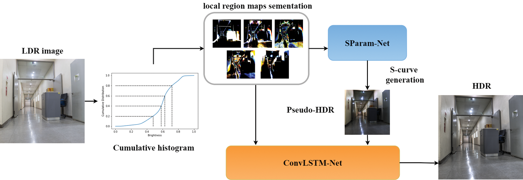
Figure 1: Proposed deep learning model
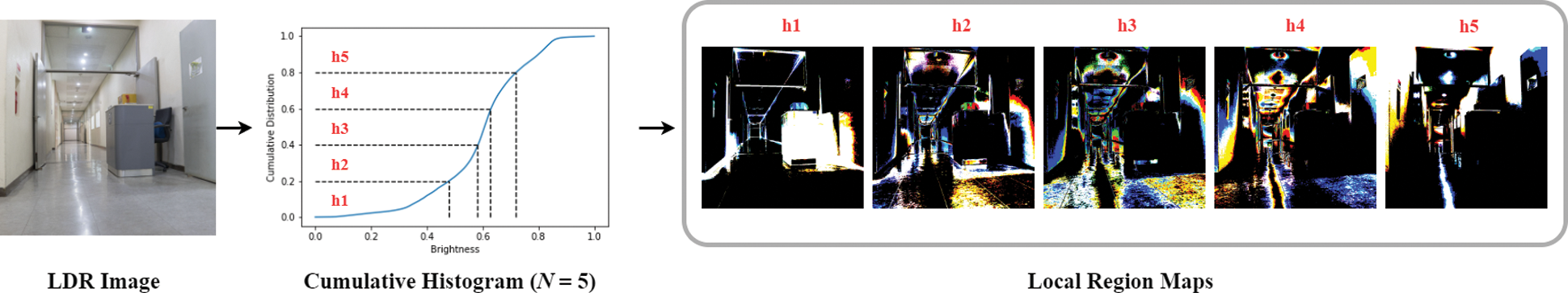
Figure 2: Local region map generation based on the cumulative histogram
Fig. 3 shows the local region maps obtained from the same scene under different exposures (EV = −2, 0, + 2). We obtained the segment region map for each color (R, G, and B) channel, and the resultant maps were concatenated in the color channels. In the figure, the maps have similar brightness distributions over three exposure values. This indicates that using the local region maps in the learning process such as inverse tone function estimation can reduce the effects associated with the exposure range of the input LDR image. Although significantly over- and/or under-exposed LDR images are inputted, the network model can effectively learn the relationship between the ground truth HDR image and input LDR image in the cumulative brightness bands.
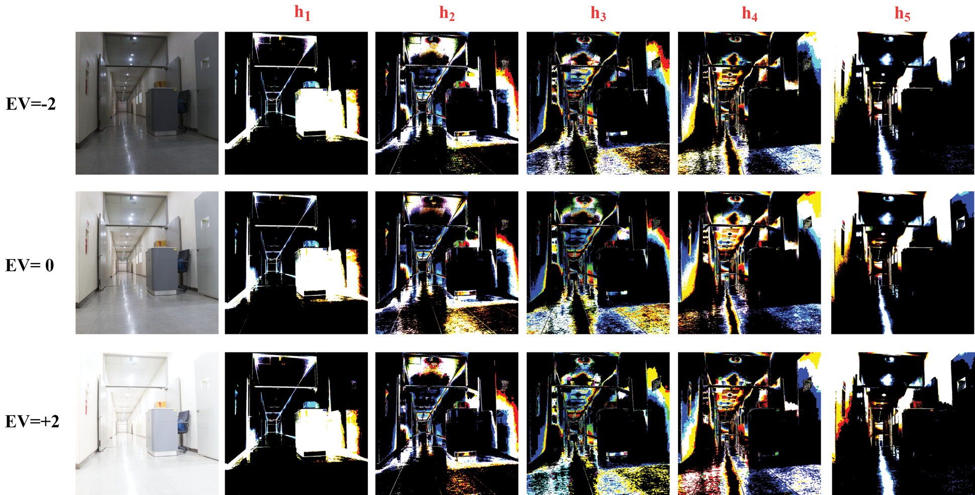
Figure 3: Local region maps from the same scene under different exposures (EV = −2, 0, + 2)
Banterle [13] developed an inverse tone mapping technique in which a world luminance Lw(x, y) is represented via a display luminance Ld(x, y), where Ld is the luminance at the pixel (x, y) in an image. The relationship between Lw and Ld has an S-like shape in a two-dimensional (2D) space; hence, it is referred to as an S-curve. This curve emphasizes both the bright and dark regions and increases the contrast of regions with intermediate brightness.
Eqs. (2) and (3) are the quadratic equation of Lw and its determinant, respectively. Here, α is a key value of the scene that indicates whether it is subjectively light, normal, or dark. Lwhite is the minimum luminance value that is mapped into a white color in the tone mapping process. This parameter also controls the contrast of the middle tone regions in the inverse tone mapping. The log-average luminance of Lw is represented as Lw_mean, which is approximated using the log-average of the luminance in the LDR image. Because Ld(x, y) always has a positive value, Lw has two different solutions. To solve the quadratic equation (Eq. (2)), we must obtain a scaling coefficient α and the maximum value L’max via inverse tone mapping. The relationship between a, L’max, Lwhite, and Lw_mean, is described in Eq. (4).
We derived a quadratic equation from Eqs. (2) and (4) and obtained the solution (Eq. (6)) by using a quadratic formula. Fig. 4 shows the input image, luminance values (blue-colored dots) of the ground truth HDR, considering the luminance values of the LDR image. The inverse tone mapping function is represented as the orange-colored line. Here, the luminance values (y-axis) are log-scaled, and L’max and Lwhite are set to 3.6 and 22, respectively. Fig. 4 shows that the LDR image can be precisely mapped into the ground truth HDR image using the S-curve generated from the user's intervention. Because the luminance does not represent the chromatic components of the LDR image, we modified the luminance channel into an RGB channel of the LDR image. Therefore, we transformed Eq. (5) into Eq. (6). Therefore, Rw, Gw, and Bw can be computed using Rd, Gd, and Bd in the LDR image. Here, Rd, Gd, and Bd are the luminance at each pixel (x, y) in the color channels.
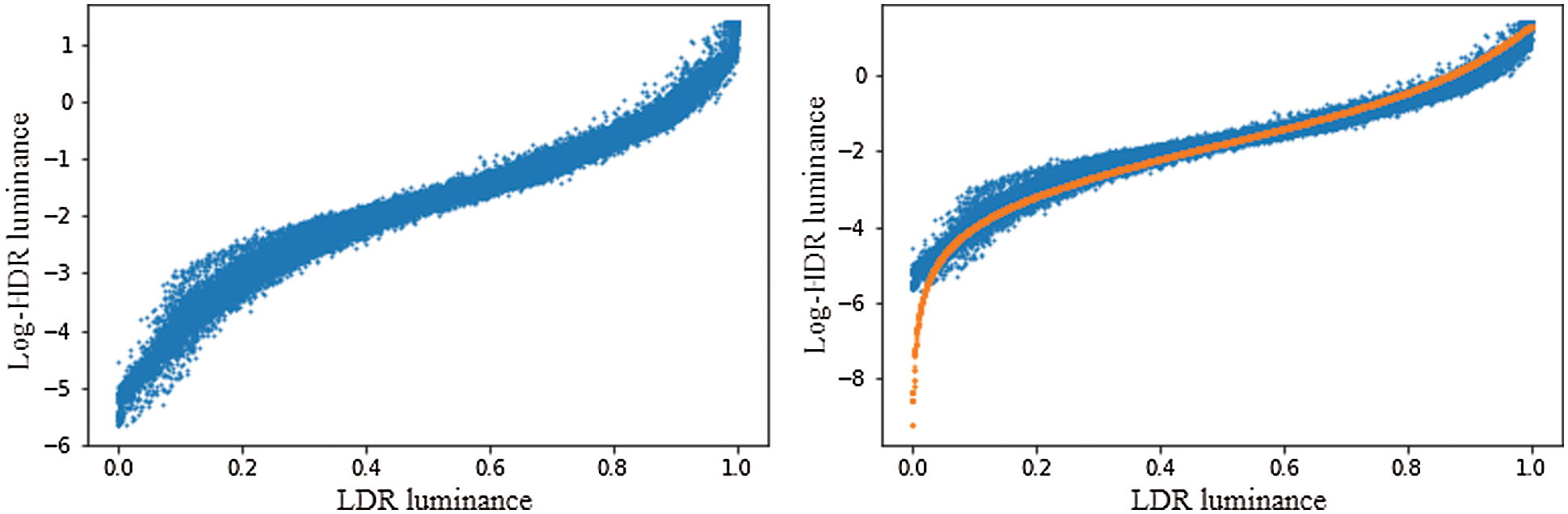
Figure 4: Log-scaled luminance values of pseudo- and ground truth HDR considering the LDR
We introduced a deep learning model, known as SParam-Net, to estimate the parameters of S-curve: L′max, Rwhite, Gwhite, and Bwhite. Using this approach, the parameters of S-curve can be estimated without relying on the parameter setting of a user, to generate a pseudo-HDR image. Fig. 5 shows the details of the SParam-Net construction process. The LDR image with a resolution of 256 × 256 and locally segmented region maps with the same resolution in the R, G, and B channels are inputted to SParam-Net. The tensor size is 256 × 256 × 18 because the total number of local region maps is five. The SParam-Net with a visual geometry group (VGG) backbone [25] has 13 convolution layers. The kernel size and stride are 3 × 3 and one. In SParam-Net, four max-pooling layers with a size of 2 × 2 (the stride is 2) were used to reduce the size of the feature map. The feature map of the final convolution layer was resized to 7 × 7 using adaptive average pooling. The final output (7 × 7 × 512) of the convolution layer map was passed through three fully connected layers. The first two layers had 4,096 nodes, and the final layer had four outputs: L′max, Rwhite, Gwhite, and Bwhite. Using S-curve with the output parameter values (Eq. (7)), the input LDR image can be mapped into the pseudo-HDR image. Further, the rectified linear unit (ReLU) function was used as an active function for the convolution and fully connected layers, and the dropout was utilized to prevent overfitting of the deep learning model.
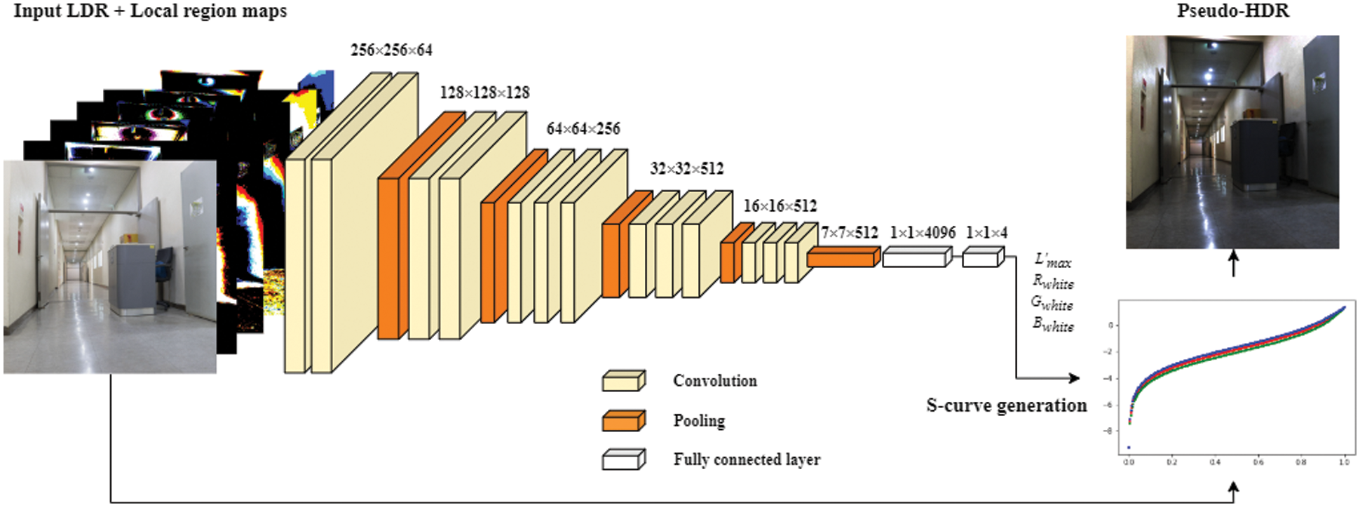
Figure 5: Details of the SParam-Net construction process
Considering the early deep learning studies on image restoration and reconstruction, the L2 loss function was employed. Zhao [26] demonstrated that a method based on the L1 loss function can reduce blurring effects compared to that based on the L2 loss function in image restoration and reconstruction. In addition, using the differentiability of the structural similarity index measure (SSIM), a loss function based on L1 and SSIM has been developed. The SSIM considers that the human visual system is sensitive to changes in the local structure [27]. In this study, the loss function (Eq. (7)) is employed in combination with L1 and SSIM during the learning process.
where PseudoHDR represents the pseudo-HDR image generated by SParam-Net and HDR represents the ground truth HDR image. In Eq. (7), a parameter, which controls the relative weights of L1 and SSIM losses, is set to 0.83.
2.2 HDR-Image Generation: ConvLSTM-Net
To generate an HDR image, the segmented local maps were sequentially inputted to ConvLSTM-Net based on the brightness. Here, the pseudo-HDR image generated using SParam-Net was also used. The LSTM is recurrent neural network architecture with feedback connections, which is well-suited for classifying and making predictions based on time-series data, such as voice and texts [28]. To obtain the convolutional structures in both the input-to-state and state-to-state transitions, a previously employed fully connected LSTM was extended to convolutional LSTM [29]. In this study, the sequentially segmented local region maps based on the cumulative histogram were considered time-dependent data inputs in the convolutional LSTM. The proposed LSTM-based model sequentially learned the local region maps, not on the time axis. However, it learned those on the cumulative brightness distribution, considering the global inverse tone mapping. The proposed approach is the first example of the processing of the sequentially segmented maps in the convolutional LSTM.
ConvLSTM-Net is composed of two parts: an encoder and a decoder. The encoder extracts the relationship of the local brightness distribution in each brightness band, which is divided using the cumulative histogram and global luminance of the pseudo-HDR image. Deconvolution operation is performed on the feature map with the lower resolution to reconstruct the feature map with the same resolution as the input LDR image [19,22]. Previous encoders based on U-Net [30] cause images to be distorted by checkerboard artifacts owing to the upsampling layers [31,32]. The proposed approach is not encumbered by checkerboard artifacts because neither the upsampling nor the downsampling layers are employed.
The convolution operation of ConvLSTM-Net is represented as Conv(fi, ni, ci), where fi, ni, and ci represent the size of the convolution kernel, number of output, and input channels, respectively. The convolutional LSTM with two layers, namely, Conv(3, 64, 6) and Conv(3, 6, 64), was used as the encoder. As previously indicated, the local region maps were obtained from the relatively bright regions close to the dark local regions, based on the order of brightness. Both the pseudo-HDR image obtained via S-param Net and segmented region maps were sequentially forwarded to each cell of the convolutional LSTM. Because the LDR image is non-linearly mapped to the camera response function, learning a direct HDR mapping from a single LDR image is difficult. The proposed model can effectively learn their relationship by using the HDR image and sequentially segmented local regions based on the order of brightness.
The encoded feature map was transferred into the decoder to reconstruct the HDR image. We employed the FSRCNN, which was constructed using feature extraction, shrinking, mapping, expanding, and deconvolution processes [33]. First, the feature map was extracted from the input tensor using the Conv(5, 64, 6) operation. Second, the dimension of the feature map was reduced using Conv(1, 12, 64). The mapping process performed four Conv(3, 12, 12) operations and non-linear active functions, learning the non-linear mapping. Considering the expanding process, the decreased dimension was expanded using the Conv(1, 64, 12) operation. Regarding the deconvolution process, the previously developed FSRCNN model increased the dimension of the feature map to generate a super-resolution image. Because the dimensions of the input image and those of the output are the same, the HDR image can be reconstructed using DeConv(9, 3, 64) with one stride. The parametric ReLU active function was employed after every convolution operation of the decoder. The ReLU function was used in the final deconvolution operation. The loss function, defined using L1 and SSIM measures, computes the errors between the output HDR image generated by the ConvLSTM-Net and ground truth HDR. Fig. 6 presents the details of the ConvLSTM-Net construction process.
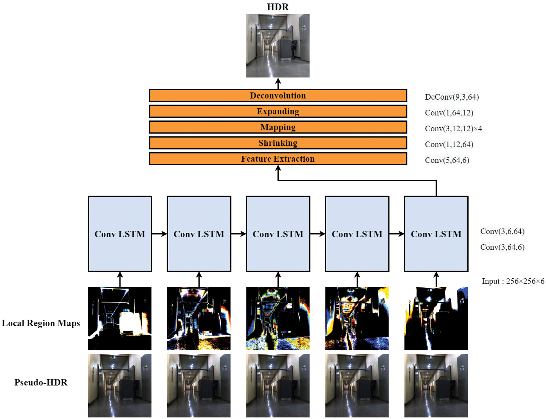
Figure 6: Details of the ConvLSTM-Net construction process
The proposed network model, which was constructed using the SParam-Net and ConvLSTM-Net, was jointly learned for HDR reconstruction from a single image. SParam-Net was learned to estimate the inverse tone mapping function. The weight values of SParam-Net were used as the initial weight values of the proposed model during the learning process. The final loss function was defined as Eq. (8).
where LossLstm and LossSParam represent the losses by ConvLSTM-Net and SParam-Net, respectively. Here, α and β are the relative weight values of the two loss values.
In this experiment, HDR-Real [21], LDR-HDR pair [20], and HDR-Eyes [34] datasets were used in learning and training processes. The HDR-Real dataset images were captured using 42 cameras, including NIKON D90, NEX-5N, and Canon EOS 6D with multiple exposures. Bracketed image pairs comprising 5–20 images of the same scene were used for HDR image generation. The dataset included 820 HDR and 9,786 LDR images. The LDR-HDR pair datasets were captured using a Samsung NX3000 camera in an auto-exposure bracket mode (EV = −2, 0, 2) at a resolution of 1024 × 1024 pixels. Three images of the 450 scenes of several categories (e.g., indoor, outdoor, landscape, objects, buildings, and nights) were obtained at different exposures and merged into an HDR image using the Pro algorithm [3]. The HDR-Eye dataset was built by combining nine bracketed images that were acquired using several cameras, including Sony DSC-RX100 II, NEX-5N, and α6000, with different exposure settings (EV = −2.7, −2, −1.3, −0.7, 0, 0.7, 1.3, 2, 2.7) [34]. Regarding the three datasets, 970 HDR and 10,236 LDR images were randomly chosen as the training dataset, and 346 HDR and 946 LDR images were chosen as the test dataset.
The LDR images were represented based on the dynamic range of a pixel (8-bit) (i.e., [0, 255]). Generally, because different HDR-images have different dynamic ranges and maximum values, normalization of the dataset is required to ensure an effective learning performance. In addition, if the luminance values of the HDR-images are normalized with the maximum value in the range of [0, 1], many pixels in the image have near-zero values. This is because the HDR image has a large dynamic range, and the size of the bright regions is generally small. The network finds it difficult to learn to reconstruct HDR-images that have quite small pixel values. Prior to the learning process in our network model, the average pixel value of the HDR image was normalized to 0.5.
There are many image quality assessment methods for the evaluation of the performance of inverse tone mappings [12,20,21,35,36]. High dynamic range visible difference predictor 2 (HDR-VDP-2) estimates the probability that an average human observer will detect the difference and quality between a pair of images [12]. Because HDR-VDP-2 is based on the visual model for all the luminance conditions, this measure is used to evaluate the accuracy of HDR reconstruction. In addition, the peak signal-to-noise ratio (PSNR) and SSIM metrics are widely employed. Both the reconstructed HDR and reference ground-truth HDR-images were normalized using a previously reported processing step [18]. We used PSNR and SSIM to evaluate the tone-mapped HDR-images and determined the average scores from four tone-mapping operators: Balanced, Smooth, Enhanced, and Soft in Photomatix [21].
To train and test our proposed deep learning model, we conducted experiments on a computer equipped with a Core i5-9600k CPU, 16 GB RAM, and GeForce GTX 1080Ti GPU, and we used Python language and PyTorch deep learning library. Our network model has been implemented and performed in the commercial computer system, considering the computation and memory complexity. We trained our model with a stochastic gradient descent of a batch size of four using the Adam optimizer (β_1 and β_2: 0.9 and 0.999, respectively) with a fixed learning rate of 7e-5. When an input image size is 256 × 256, SParam-Net has 134.28 M weight parameters and 20.79 giga floating operations per second (GFLOPs), and ConvLSTM-Net has 0.21 M parameters and 59.07 GFLOPs. The total number of the proposed model is 134.49 M and has 79.86 GFLOPs. The LSTM network maintains a low number of parameters by weight sharing; nonetheless, its operation is performed iteratively across the input sequences. Therefore, unlike Sparam-Net, ConvLSTM-Net has fewer parameters and more computation load (GFLOPs).
In our experiment, the proposed network model was converged after training for 50 epochs. SParam-Net was trained to generate the global inverse tone mapping from the local region maps. The trained weight parameters of SParam-Net were used as the initial values in joint learning of SParam-Net and ConvLSTM-Net. It took 10 min to train SParam-Net and 18 min per epoch for the joint training our model (SParam-Net and ConvLSTM-Net). The running time at inference in our network model is approximately 76 ms for 256 × 256 images and 262 ms for 512 × 512 images.
First, the luminance distribution of the ground truth HDR image was compared to that of the pseudo-HDR image that was generated using the inverse tone mapping function via SParam-Net. Because these luminance values were obtained in the color channels, the pixel values could be evaluated without considering additional chromatic components [20]. Fig. 7 shows the log-scaled luminance values of an HDR image, considering the luminance values of the LDR image. The inverse tone mapping function estimated by SParam-Net is represented by the orange-colored line in Fig. 4. Fig. 7 also shows that the estimated inverse tone mapping function adequately represents the relationship between the HDR and LDR luminance values. Considering the input LDR image captured using a low aperture value, the estimated inverse tone mapping function exhibited more differences compared to other cases.
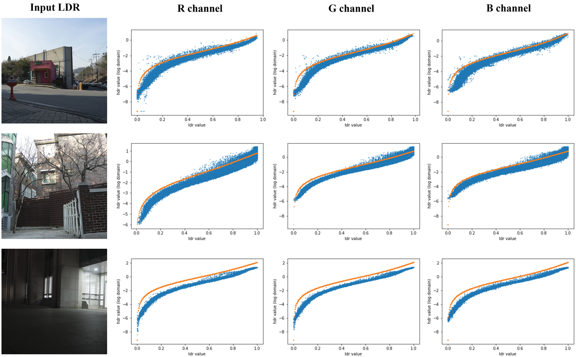
Figure 7: Log-scaled luminance values of the estimated pseudo-HDR and ground truth HDR considering the LDR
The proposed model was compared to contemporary deep learning-based methods: Expand-Net [18], DrTMO [19], HDRCNN [22], SingleHDR [21]), using HDR-VDP-2, PSNR, and SSIM as the evaluation metrics. These methods were implemented using codes by the authors and open sources. In Tab. 1, the median values and variation ranges for HDR-VDP-2, PSNR, and SSIM metrics for the HDR-Real, LDR-HDR-pair, and HDR-Eye datasets are presented, considering the relative weight values (α and β) of SParam-Net and ConvLSTM-Net. When the relative weight (α) of ConvLSTM-Net is larger than that of SParam-Net (β), the proposed model provides a better performance as shown in Tab. 1. This implies that sequential learning of the details in local region maps based on the global luminance distribution is more effective than the estimation of the inverse tone mapping.
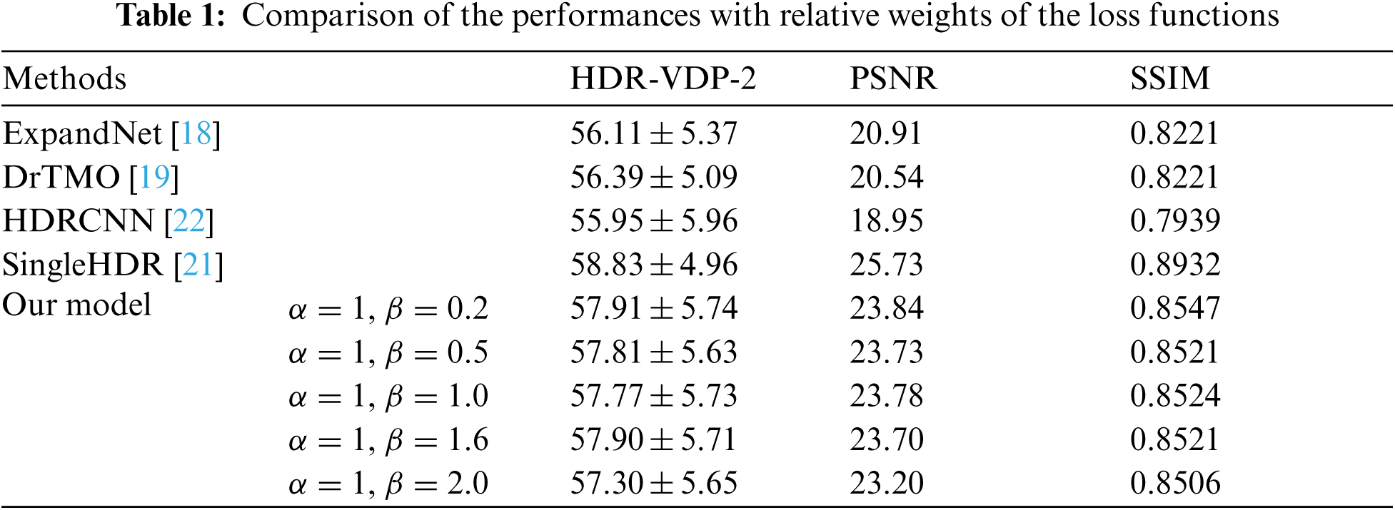
The proposed method achieved a comparable performance, considering the other three methods (Expand-Net, DrTMO, HDRCNN) except for SingleHDR to some extent. SingleHDR utilizes three CNNs for the sub-tasks of dequantization, linearization, and hallucination [21]. The proposed model sequentially learns the correlation between the global luminance distribution and local regions based on the cumulative brightness distribution. In this study, both the correction of the quantization errors and the reconstruction of the details in over-exposed regions are considered implicitly. If additional considerations about the over- and/or under-exposed information are included, the performance can be further improved. Tab. 2 shows the performance over the total number (N) of the segmented local region maps, which is the divisor of the cumulative histogram. In Tab. 2, the best performance is obtained when N is 5.

Fig. 8 shows the resultant HDR images obtained using the contemporary approaches, compared to those generated using the proposed method. The results are tone-mapped to facilitate qualitative evaluation. To better compare the results, the areas identified using the red-colored square are enlarged. In the bright regions of Figs. 8a and 8c and the dark regions of Fig. 8b, the details of the image are more precisely reconstructed, and the resultant HDR-images are more visually appealing. Regarding the results generated by the ExpandNet and DrTMO methods, the color tones of the reconstructed results are different from that of the ground truth HDR image (GT in Fig. 8). By estimating the inverse tone mapping function in the R, G, and B channels, the proposed method can more precisely reconstruct the ground truth HDR color.
The following is the summary of the main contributions of this paper: 1) The local region maps, which are segmented based on the cumulative brightness distribution, are used to estimate an inverse tone mapping function. 2) The globally tone mapped-local region maps are used as the input sequences on the LSTM model for HDR image reconstruction. In our network model, the correlation of the brightness distribution in the local region maps and the global luminance distribution of the pseudo-HDR image can be encoded. However, the proposed model still encounters difficulty in reconstructing over and/or under-exposed regions. Therefore, we need to further consider scattered noise or contouring artifacts that occurred often in the quantization process.
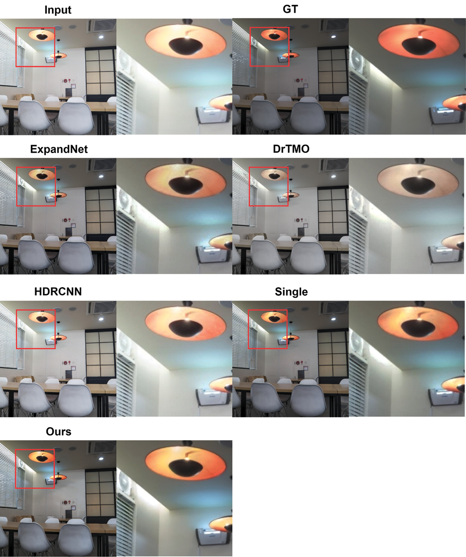
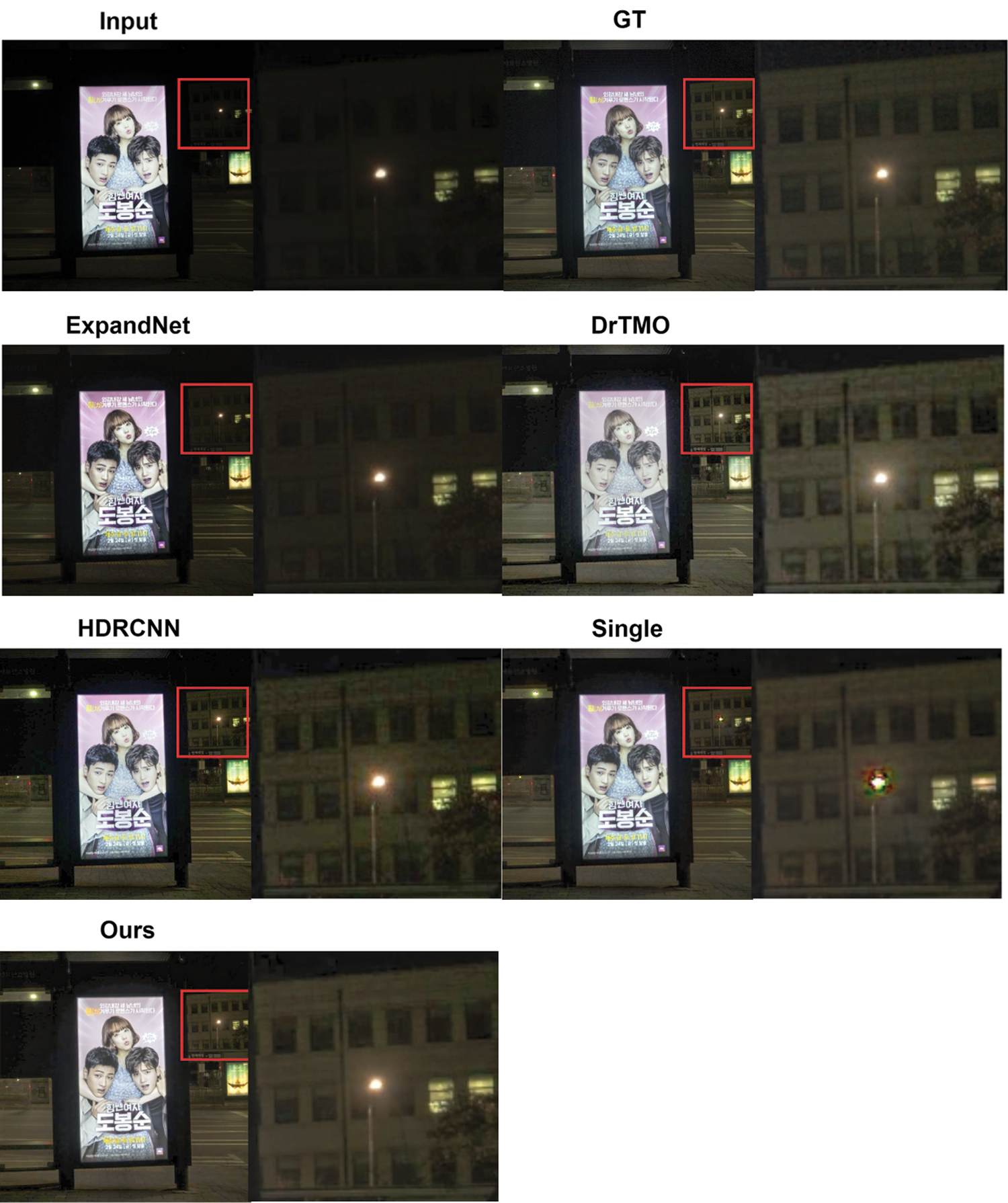

Figure 8: (a) Comparison of the HDR-images by the contemporary methods and proposed approach
In this paper, we presented a deep learning model for reconstructing an HDR image from a single LDR image. SParam-Net was used to estimate the inverse tone mapping function to generate a pseudo-HDR image. Both the pseudo-HDR image and segmented local region maps based on the cumulative histogram were inputted sequentially into the convolutional LSTM. The weights obtained from the SParam-Net were transferred for joint learning of the end-to-end reconstruction model. It was demonstrated that based on the order of the brightness values obtained from the LDR image, the local region maps can be effectively used in the convolutional LSTM to learn the relationship between the LDR and HDR images. Therefore, the model can sequentially learn the details of the brightness bands, considering the global luminance distribution. The proposed model was compared to contemporary deep learning-based methods based on HDR-VDP-2, PSNR, and SSIM measures. The results of the experiments show that the proposed deep learning model can reconstruct an HDR image from a single LDR image more reliably than the contemporary end-to-end methods. However, the proposed model still encounters difficulty in reconstructing over and/or under-exposed regions. Further considerations on the scattered noise or contouring artifacts that occur often in the quantization process are needed.
Funding Statement: This study was supported by the Basic Science Research Program through the National Research Foundation of Korea (NRF) funded by the Ministry of Education (NRF-2018R1D1A1B07049932).
Conflicts of Interest: The authors declare that they have no conflicts of interest to report regarding the present study.
1. A. Adams, The Camera (The Ansel Adams Photography Series). Little, Brown and Company, New York City, 1981. [Google Scholar]
2. E. Reinhard, G. Ward, S. Pattanaik and P. Debevec, High Dynamic Range Imaging: Acquisition, Display, and Image-Based Lighting. Morgan Kaufmann, Amsterdam, 2010. [Google Scholar]
3. P. E. Debevec and J. Malik, “Recovering high dynamic range radiance maps from photographs,” in Proc. ACM SIGGRAPH, LA, CA, USA, pp. 1–10, 2008. [Google Scholar]
4. S. Nayar and T. Mitsunaga, “High dynamic range imaging: Spatially varying pixel exposures,” in Proc. Conf. on Computer Vision and Pattern Recognition, Head Island, SC, USA, pp. 472–479, 2000. [Google Scholar]
5. S. Silk and J. Lang, “Fast high dynamic range image deghosting for abitrary scene motion,” in Proc. Conf. on Graphics Inerface, Toronto, Canada, pp. 85–92, 2012. [Google Scholar]
6. E. A. Khan, A. O. Akyuz and E. Reinhard, “Ghost removal in high range images,” in Proc. Int'l. Conf. on Image Processing, Atlanta, GA, USA, pp. 2005–2008, 2006. [Google Scholar]
7. J. Kronader, S. Gustavson, G. Bonnet and J. Unger, “Unified hdr reconstruction from raw cfa data,” in Proc. IEEE Int'l. Conf. on Computational Photography, Cambridge, MA, USA, pp. 1–9, 2013. [Google Scholar]
8. M. D. Tocci, Ch. Kiser, N. Tocci and P. Sen, “A versatile hdr video production system,” ACM Transactions on Graphics, vol. 30, no. 4, pp. 1–10, 2011. [Google Scholar]
9. P. Didyk, R. Mantiuk, M. Hein and H. P. Seidel, “Enhancement of bright video features for hdr displays,” Compt. Graphics Forum, vol. 27, no. 4, pp. 1265–1274, 2008. [Google Scholar]
10. T. Wang, C. Chiu, W. Wu, J. Wang, C. Lin et al., “Pseudo-multiple-exposure-based tone fusion with local region adjustment,” IEEE Transactions on Multimedia, vol. 17, no. 4, pp. 470–484, 2015. [Google Scholar]
11. F. Banterle, P. Ledda, K. Debattista and A. Chalmers, “Inverse tone mapping,” in Proc. Computer Graphics and Interactive Techniques, Kuala Lumpur, Malaysia, pp. 349–356, 2006. [Google Scholar]
12. R. Mantiuk, K. J. Kim, A. G. Rempel and W. Heidrich, “Hdr-vdp-2: A calibrated visual metric for visibility and quality predictions in all luminance conditions,” ACM Transactions on Graphics, vol. 30, no. 4, pp. 1–14, 2011. [Google Scholar]
13. B. Masia, S. Agustin, R. W. Fleming, O. Sorkine and D. Gutierrrez, “Evaluation of reverse tone mapping through varying exposure conditions,” in Proc. Sigraph Asia, Yokohama, Japan, pp. 1–8, 2009. [Google Scholar]
14. L. Wang, L. Y. Wei, K. Zhou, B. Guo and H. Y. Shum, “High dynamic range image hallucination,” in Proc. Eurographics Conf. on Rendering Techniques, Grenoble, France, pp. 321–326, 2007. [Google Scholar]
15. E. Reinhard, M. Stark, P. Shirley and J. Ferwerda, “Photographic tone reproduction for digital images,” ACM Transactions on Graphics, vol. 21, no. 3, pp. 267–276, 2002. [Google Scholar]
16. A. G. Rempel, M. Trentacoste, H. Seetzen, H. D. Young, W. Heidrich et al., “Ldr2hdr: On-the-fly reverse tone mapping of legacy video and photographs,” ACM Transactions on Graphics, vol. 26, no. 3, pp. 39–1–39–5, 2007. [Google Scholar]
17. J. Zhang and J. F. Lalonde, “Learning high dynamic range from outdoor panoramas,” in Proc. IEEE Int. Conf. on Computer Vision, Venice, Italy, pp. 4519–4528, 2017. [Google Scholar]
18. D. Marnerides, T. Bashford-Rogers, J. Hatchett and K. Debattista, “Expandnet: A deep convolutional neural network for high dynamic range expansion from low dynamic range content,” Computer Graphics Forum, vol. 37, no. 2, pp. 37–49, 2018. [Google Scholar]
19. Y. Endo, Y. Kanamori and J. Mitani, “Deep reverse tone mapping,” ACM Transactions on Graphics, vol. 36, no. 6, pp. 177: 1–177:10, 2017. [Google Scholar]
20. H. Jang, K. Bang, J. Jang and D. Hwang, “Dynamic range expansion using cumulative histogram learning for high dynamic range image generation,” IEEE Access, vol. 8, pp. 38554–38567, 2020. [Google Scholar]
21. Y. Liu, W. Lai, Y. Chen, Y. Kao, M. Yang et al., “Single-image hdr reconstruction by learning to reverse the camera pipeline,” in Proc. Conf. on Computer Vision and Pattern Recognition, Seattle, WA, USA, pp. 1651–1660, 2020. [Google Scholar]
22. G. Eilertsen, J. Kronander, G. Denes, R. K. Mantiuk and J. Unger, “Hdr image reconstruction from a single exposure using deep cnns,” ACM Transactions on Graphics, vol. 36, no. 6, pp. 1–15, 2017. [Google Scholar]
23. X. Chen, Y. Liu, Z. Zhang, Y. Qiao, C. Dong, “HDRUnet: Single image hdr reconstruction with denoising and dequantization,” in Proc. Conf. on Computer Vision and Pattern Recognition, Virtual, pp. 354–363, 2021. [Google Scholar]
24. N. K. Kalantari and R. Ramamoorthi, “Deep high dynamic range imaging of dynamic scenes,” ACM Transactions on Graphics, vol. 36, no. 4, pp. 144 :1–144:12, 2017. [Google Scholar]
25. K. Simonyan and A. Zisserman, “Very deep convolutional networks for large-scale image recognition,” in Proc. Int'l. Conf. on Learning Representations, San Diego, CA, USA, pp. 1–14, 2015. [Google Scholar]
26. H. Zhao, O. Gallo, I. Frosio and J. Kautz, “Loss functions for image restoration with neural networks,” IEEE Transactions on Computational Imaging, vol. 3, no. 1, pp. 47–57, 2017. [Google Scholar]
27. Z. Wang, A. C. Bovik, H. R. Sheikh and E. P. Simoncelli, “Image quality assessment: From error visibility to structural similarity,” IEEE Transactions on Image Processing, vol. 13, no. 4, pp. 600–612, 2004. [Google Scholar]
28. S. Hochreiter and J. Schmidhuber, “Long short-term memory,” Neural Computation, vol. 9, no. 8, pp. 1735–1780, 1997. [Google Scholar]
29. X. Shi, Z. Chen, H. Wang, D. Yeung, W. Wong et al., “Convolutional lstm network: A machine learning approach for precipitation nowcasting, in Proc. Int'l. Conf. on Neural Information Processing Systems, Montreal, Canada, pp. 802–810, 2015. [Google Scholar]
30. O. Ronneberger, P. Fischer and T. Brox, “U-Net: Convolutional networks for biomedical image segmentation,” LNCS, vol. 9351, pp. 234–241, 2015. [Google Scholar]
31. Y. Sugawara, S. Shiota and H. Kiya, “Super-resolution using convolutional neural networks without any checkerboard artifacts,” in Proc. Int'l. Conf. Image Processing, Athens, Greece, pp. 66–70, 2018. [Google Scholar]
32. Y. Kinoshita and H. Kiya, “Fixed smooth convolutional layer for avoiding checkerboard artifacts in cnns,” in Proc. IEEE Int. Conf. Acoust. Speech Signal Process, Virtual Barcelona, pp. 3712–3716, 2020. [Google Scholar]
33. C. Dong, C. Loy and X. Tang, “Accelerating the super-resolution convolutional neural network,” in Proc. of European Conf. on Computer Vision, Amsterdam, Netherlands, pp. 391–407, 2016. [Google Scholar]
34. H. Nemoto, P. Korshunov, P. Hanhart and T. Ebrahimi, “Visual attention in ldr and hdr images,” in Proc. of Int.’l Workshop on Video Processing and Quality Metrics for Consumer Electronics, Chandler, Arizona, USA, pp. 1–6, 2015. [Google Scholar]
35. S. Lee, G. An and S. Kang, “Deep recursive hdri: Inverse tone mapping using generative adversarial networks,” in Proc. European Conf. on Computer Vision, Munich, Germany, pp. 596–611, 2018. [Google Scholar]
36. T. O. Aydin, R. Mantiuk and H. P. Seidel, “Dynamic range independent image quality assessment,” ACM Transactions on Graphics, vol. 27, no. 3, pp. 1–10, 2008. [Google Scholar]
 | This work is licensed under a Creative Commons Attribution 4.0 International License, which permits unrestricted use, distribution, and reproduction in any medium, provided the original work is properly cited. |