Computers, Materials & Continua DOI:10.32604/cmc.2022.022309
Article

A New Hybrid SARFIMA-ANN Model for Tourism Forecasting

Tanzila Saba1, Mirza Naveed Shahzad2,*, Sonia Iqbal2,3, Amjad Rehman1 and Ibrahim Abunadi1

1Artificial Intelligence & Data Analytics Research Lab (AIDA), CCIS Prince Sultan University, Riyadh, 11586, Saudi Arabia
2Department of Statistics, University of Gujrat, Gujrat, 50700, Pakistan
3Department of Statistics, University of Sialkot, Sialkot, 51310, Pakistan
*Corresponding Author: Mirza Naveed Shahzad. Email: nvd.shzd@uog.edu.pk
Received: 03 August 2021; Accepted: 29 October 2021

Abstract: Many countries developed and increased greenery in their country sights to attract international tourists. This planning is now significantly contributing to their economy. The next task is to facilitate the tourists by sufficient arrangements and providing a green and clean environment; it is only possible if an upcoming number of tourists’ arrivals are accurately predicted. But accurate prediction is not easy as empirical evidence shows that the tourists’ arrival data often contains linear, nonlinear, and seasonal patterns. The traditional model, like the seasonal autoregressive fractional integrated moving average (SARFIMA), handles seasonal trends with seasonality. In contrast, the artificial neural network (ANN) model deals better with nonlinear time series. To get a better forecasting result, this study combines the merits of the SARFIMA and the ANN models and the purpose of the hybrid SARFIMA-ANN model. Then, we have used the proposed model to predict the tourists’ arrival in New Zealand, Australia, and London. Empirical results showed that the proposed hybrid model outperforms in predicting tourists’ arrival compared to the traditional SARFIMA and ANN models. Moreover, these results can be generalized to predict tourists’ arrival in any country or region with a complicated data pattern.

Keywords: SARFIMA; hybrid model; tourists’ arrival forecasting; ANN

1  Introduction

The rapid development in the tourism industry in the last 30 years has contributed to many countries’ economies. According to the World Travel & Tourism Council (WTTC), 2019, tremendous evolution was observed in the tourism industry. It has created 313 million jobs and created prosperity in industries related to tourism and has increased taxations. As a result, the tourism industry had generated 10.3% of the global GDP. Consequently, every country is paying much attention to growing tourists’ arrival in their territory. Therefore, tourism policy makers and business practitioners are interested in knowing an accurate forecast of tourist volume for properly distributing resources and formulating pricing strategies [1].

One well-known approach to model tourists’ arrival data is to use time series models. For this purpose, models based on the Box-Jenkins methodology have been extensively used in the past several decades. For example, the autoregressive integrated moving average (ARIMA) and its sub-models are well-recognized to predict future observations based on linearly correlated past observation and a white noise error term. However, these models work efficiently only for short memory time series processes [2]. On the other hand, most time-series data, including financial data, stock-exchange data, and numbers of tourists’ arrivals, have long memory characteristics. For such types of time series data, Granger [3] introduced the autoregressive fractional integrated moving average (ARFIMA) model that speculates the ARIMA by allowing non-integer values of the differencing parameter (d). Recall, Robinson [4], that the long memory in time series is termed autocorrelation at long lags, and the strength of this long memory is measured by d of the ARFIMA model.

The ARFIMA model has been applied in several studies for accurate forecasting. For example, Doornik et al. [5] forecasted US and UK inflation rates using the ARFIMA model and showed its superiority over the ARIMA model. Chu [6] has found better forecasting about tourists’ demand in Hong Kong, Japan, and Korea by ARFIMA model than ARIMA. Moreover, Cheung [7] used the ARFIMA model for predicting the foreign exchange rates. Along with the ARFIMA model, Prass et al. [8] also applied the seasonal autoregressive fractional integrated moving average (SARFIMA) model to predict the mean monthly water level Paraguay River in Brazil. The SARFIMA model has also been used by Mostafaei et al. [9] to predict Iran's oil supply. In recent years, Peng et al. [10] developed the new hybrid random forest-LSTM model to forecast tourist arrival data and justified by the Beijing city and Jiuzhaigou valley data that this hybrid approach outperforms. Waciko et al. [11] used the Thief-MLP hybrid approach to forecast short-term tourists’ arrival to Bali-Indonesia. Wu et al. [12] forecasted daily tourist arrival to Macau SAR, China with a hybrid SARIMS–LSTM approach and obtained the good fitted results.

It is important to note that all Box-Jenkins models require the linearity of the process under study (see, e.g., [13]). This means that future observations should have a linear relationship with present and past observations. Therefore, ARFIMA and SARFIMA models become inappropriate when time series are generated from nonlinear processes. Nonlinear models such as the Artificial Neural network (ANN) have been used in several studies to overcome this problem. For instance, Sarvareddy et al. [14] studied the characteristics of ANN and showed its forecasting power over traditional time series models. Zhang et al. [15] studied ANN forecasting for seasonal and trend time series and showed that the ANN has nonlinear architecture and performs well for linear time series. In several studies, ANN has been constantly compared with the traditional Box-Jenkins model and long memory models, and its better performance is justified. Prybutok et al. [16] observed that the ANN analysis performs better for time series datasets, specifically in the presence of nonlinearity.

Note that there is no definitive proper measure to check whether the process generated from time series is linear or nonlinear. Therefore, it would be difficult to decide in advance which model should be used. Furthermore, there is no standard model that is appropriate for both linear and nonlinear time series data. Therefore, by combining the characteristics of two or more models, the accuracy can be increased. Different hybrid models have been developed following this idea, particularly by combining linear autoregressive models and ANN models. The beauty of these types of hybrid models is that they can capture the characteristics of both linearity and non-linearity in the time series [17]. This idea was first used by Zhang [18] to introduce a hybrid methodology that combines both ARIMA and ANN models. Following [18], a hybrid of ARIMA models and support vector machines (SVMs) were used by Pai et al. [19] to forecast stock prices. Chen et al. [20] examined the forecasting accuracy of the hybrid of seasonal ARIMA (SARIMA) and SVM models for Taiwan's machinery industry production. Chaâbane [21] found a hybrid of ARFIMA and ANN model more efficient over individual ARFIMA and ANN to predict electricity price.

Moreover, Chaâbane [22] found a better performance of hybrid ARFIMA–least-squares SVM than the competing models while predicting electricity spot prices. In general, practitioners rely on two methods to forecast tourist volume. One is time series analysis methods [23] and the other is artificial intelligence methods [24–26]. However, many recent studies have proved that the combination of the aforementioned methods leads to better forecasts [27–29].

In the present study, our main interest is to introduce a new hybrid model for better and accurate prediction using the complicated time series data, the new hybrid model is proposed by hybridizing the SARFIMA and ANN model using the Zhang [18] approach. The second goal is to evaluate the predictability of the developed model on the different natured tourists’ arrival datasets, for this, the datasets of the three countries were retrieved and better results have been obtained. Finally, the performance of the suggested model is verified using out-of-sample data as real-time analysis, and the results predicted by the model matched with the real tourists’ arrival values.

The rest of the paper is organized as follows. An overview of ARFIMA, SARFIMA, and ANN models is given in Sections 2, 3, and 4, respectively. The proposed hybrid SARFIMA-ANN model is presented in Section 5. Section 6 reports on the proposed hybrid model's empirical results using three real datasets on tourists’ arrival and discussion. The concluding remarks are given in Section 7.

2  ARFIMA (p,d,q) Model

When there is a long memory presence in time series data, the frequently used model is the ARFIMA model, introduced by Granger et al. [30] and its properties were further investigated by Baillie [31]. Let us assume that {yt}t∈W is a stationary process with the white noise error term εt with zero mean and variance σ2>0. Let B be the backshift operator defined by Bk(yt):=yt−k. Further, assume that {yt}t∈W is a linear process satisfying the following relationship

ψ(B)(1−B)dyt=ϑ(B)εt,t∈W,(1)

where d∈(−0.5,0.5), ψ(⋅) and ϑ(⋅) are the following polynomials of degree p and q respectively, that is

ψ(B):=1−ψ1(B)−ψ2(B2)⋯ψp(Bp),

ϑ(B):=1−ϑ1(B)−ϑ2(B2)⋯−ϑq(Bq),

where ψk,1≤k≤p and ϑl,1≤l≤q are real constant terms. Then the series {yt}t∈W follows a fractional differencing model ARFIMA (p,d,q). Note that the ARFIMA (p,d,q) model is an improved form of the traditional ARIMA (p,d,q) model due to considering fractional differencing parameter d. If d∈ (−0.5, 0.5), the series {yt}t∈W satisfies the property of stationary and inevitability and indicates a long memory process. On the other hand, d=0 indicates a short memory, whereas d∈ (−0.5, 0) tells that the process has an intermediate memory level.

3  SARFIMA (p,d,q)(P,D,Q)s Model

There are several situations in which time-series data have a long memory and exhibit periodic patterns. The appropriate model for such time-series data is the SARFIMA (p,d,q)(P,D,Q)s, an extended form of the ARFIMA process [32]. The following are propositions that need to be satisfied to consider SARFIMA as an appropriate model.

Proposition 1: Let {yt}t∈W be the stochastic stationary process following spectral density function fy(.). Suppose that there is a real quantity t∈(0, 1), a constant Cf and K∈[0,π] (with one or a finite number of occurrences) such that fy(ω)∼Cf|ω−K|−t When ω → G. Then {yt}t∈W follow a long memory process.

When t ∈ (−1, 0), then the process yt is said to be an intermediate memory process [33].

Proposition 2: Let {yt}t∈W be a seasonal stationary process with

ψ(B)ζ(Bs)(1−B)dyt=ϑ(B)ϱ(Bs)εt(2)

where εt is a white noise process with zero mean and variance σ2>0, s is the seasonal period, ΔsD=(1−BS)D is the seasonal difference operator, ψ(.),ζ(.), ϑ(.) and ϱ(.) are the polynomials of degrees p,q,P, and Q respectively defined by

ψ(B)=∑k=0p⁡(−ψk)Bkϑ(B)=∑h=0Q⁡(−ϑh)Bh

ζ(B)=∑l=0P⁡(−ζl)Blϱ(B)=∑g=0q⁡(−ϱg)Bg

where ψk,1≤k≤p,ϑh,1≤l≤Q,ζl,1≤l≤P,andϱg,1≤g≤Q are constant integers with ψ0=ζ0=ϑ0=ϱ0=−1.

Proposition 3: Assume that {yt}t∈W is the SARFIMA (p,d,q)(P,D,Q)s process, with mean zero and seasonal period s∈N. Suppose ψ(W)ζ(Ws)=0 and ϑ(W)ϱ(Ws)=0, have no zero in common. Then, the following axioms are factual:

i.   The process {yt}t∈W follows the stationary process when D<0.5, (d+D)<0.5, and ψ(W)ζ(Ws)≠0 for |W|≤1.

ii.   The stationary process {yt}t∈W follows long memory process when (d+D)∈(0,0.5), D∈(0,0.5) and ϑ(W)ϱ(Ws)≠0 for |W|≤1.

iii.   The stationary process {yt}t∈W follows long memory process when (d+D)∈(−0.5,0.5), D∈(−0.5,0) and ψ(W)ζ(Ws)≠0 for |W|≤1.

Based on Katayama's previous work [34], model estimation using SARFIMA requires a few steps. Firstly, identifying the long memory process and finding fractional difference parameter d. Secondly, identifying the model and estimating parameters, and finally, applying some diagnostic checks. After obtaining a suitable model, it can be used for predictive purposes.

4  Artificial Neural Network Based Forecasting

When the restriction of linearity on time series data is relaxed, enormous nonlinear models have been developed for obtaining better forecasts. An artificial neural network (ANN) is one of them. The critical characteristic of ANN over other nonlinear models is its ability to deal with a large class of functions. Moreover, ANN does not require any prior assumption for the estimation process. Instead, its architecture is entirely determined from the characteristic of data. For more details on ANN, we refer the interested readers to [35].

The ANN architecture consists of an input layer, an output layer, and multiple hidden layers depending upon the complexity of data. Information passes through each layer in terms of neurons. For forecasting time series data (yt), the simplest neural network architecture takes lagged values (yt−1,yt−2,yt−3,….,yt−p) as input. We used the Rabie et al. [36] heuristic/Ad-hoc input selection criteria to select the input nodes for ANN. Then the nonlinear relationship between output yt and input values (yt−1,yt−2,yt−3,….,yt−p) is defined by

yt=α0+∑j=1u⁡αjg(β0j+∑i=1v⁡βijyt−i)+εt,(3)

where εt is an error term with zero mean and standard deviation σt, αj and βij for i=0,1,2,…,v and j=0,1,2,…,u are the model parameters to be estimated. They are also known as connection weights. The function g is known as the activation function used in hidden layers to transfer the input if a certain threshold is met. One can use different activation functions like hyperbolic, sigmoid, etc. However, the most popular is the sigmoid, which is defined by

g(y)=ey1+ey.

The ANN model in (3) can be termed as univariate nonlinear autoregressive (NAR) model, that is:

yt=f(yt−1,yt−2,yt−3,….,yt−p,v)+εt(4)

Here f(.) is a function estimated by the network structure and connection weights, and v is a vector of all parameters. The ANN model (3) is quite powerful in terms of its architecture as it can estimate the arbitrary function by increasing the number of hidden nodes v.

Since there is no standard mechanism to determine the appropriate ANN architecture for the given data, multiple experiments can be conducted to choose suitable values for p and q. After selecting u and v, the model is ready for training and to estimate the network parameters.

5  Hybrid Methodology and the Proposed Hybrid Method: SARFIMA-ANN

The tourists’ arrival time series data may consist of many components such as linearity, nonlinearity, seasonality, heteroscedasticity, or a non-normal error. One standard approach for forecasting such time-series data dealing with all components does not exist. One may think SARFIMA is a better option for this case. However, SARFIMA cannot deal with complex nonlinear structures. The second choice might be the ANN, which deals well with nonlinear structure but may also provide unsatisfactory results when modeling the linear data [37]. In other words, both SARFIMA and ANN models are successful only in their domains. Zhang [18] introduced hybrid models that can model both linear and nonlinear structures of time series data to overcome this problem.

Following Zhang [18], we propose a hybrid of the SARFIMA and ANN model in this study. In the proposed model, time-series data is composed as a function of linear and nonlinear components. To be more precise, yt:=f(Nt,Lt), where Nt is termed as nonlinear part and Lt is termed as linear part. It is important to note that the hybrid approach is one of the efficient approaches that provide high accuracy rate in forecasts by establishing an additive relationship between a linear and nonlinear component of data, that is,

yt=Nt+Lt.(5)

The different methods can estimate the linear and nonlinear parts of (5) to develop the model. The defined methodology used in this work has three steps. In the first step, the linear portion of the time series data is modeled by SARFIMA, considering it follows a long memory process. From the fitted SARFIMA model, the forecasted values Lt^ are obtained. In the second step, residuals from the SARFIMA model are generated and, under the assumption that these residuals exhibit nonlinear patterns, an ANN model is trained. To be more precise, the input-output relationship is ANN is estimated by the following relationship,

et=g(et−1,et−2,et−3,….,et−p)+εt,(6)

where g(.) is a nonlinear regression function determined by the ANN model. This provides us the prediction of the nonlinear part Nt^. In the last step, predictions of the linear and nonlinear component Lt and Nt, are combined to generate the cumulative prediction, that is,

yt^=Nt^+Lt^

The pictorial representation of our proposed hybrid methodology is given in Fig. 1. In addition, the algorithm of hybrid SARFIMA-ANN is presented in Fig. 1.

Figure 1: Hybrid SARFIMA-ANN model

6  Application and Empirical Results

To check the performance of the proposed hybrid SARFIMA-ANN model on forecasting tourists’ arrival, we consider the three real data sets. As, over the past three decades, tourism has become one of the world's most flourishing industries. International tourists’ arrival has conventionally been used as a benchmark to assess any country's security condition and economic development. It significantly impacts GDP, employment rate, import and export, and many public and private sectors. This significant impact attracts the researcher to study the flow of tourists’ arrival in a particular country. The number of tourists’ arrivals can be considered a time series process due to the consistent change over time and therefore, the prediction model may be applied. Tourists’ arrival data get more attention in several studies (see, [38–40]). In this study, the following three tourists’ arrival datasets are considered to implement and justify the proposed hybrid model's competency over the other models.

Dataset 1. This dataset is related to the tourism industry, growing gradually in New Zealand due to its amazing natural attraction sites. To forecast tourists’ arrival in this country, monthly data from January 2000 to September 2018 is retrieved from https://www.stats.govt.nz, a sample of 225 observations. The plot of this dataset in Fig. 2 depicts that the considered data is stationary in the mean but has seasonal variation. The autocorrelation function and partial autocorrelation function showed the presence of seasonality at s=6.

Figure 2: Monthly data of tourists’ arrivals in New Zealand from January 2000 to September 2018

Dataset 2. The second dataset contains the monthly number of tourists’ arrival in Australia from January 2000 to August 2018, giving 224 observations, which are retrieved from https://www.abs.gov.au. The data series is regarded as nonlinear and non-Gaussian and suitable to evaluate for analysis. This time-series data has been plotted in Fig. 3, showing seasonality at s=6 with the observed trend. The data is non-stationary and the first difference is taken of the data for further analysis.

Figure 3: Monthly data of tourists’ arrivals in Australia from January 1976 to August 2018

Dataset 3. The proposed model is also applied to the number of tourists’ arrival in London, UK. The quarterly data set has 66 observations, corresponding to 2002Q1–2018Q2, taken from https://www.data.london.gov.uk and plotted in Fig. 4. There exist seasonal fluctuations at s=64 in the series. For modeling and forecasting from this series, the first difference of the data is taken.

Figure 4: Quarterly data of tourists’ arrivals (000s) in London from 2002Q1 to 2018Q2

These three datasets are used in the present study to demonstrate the effectiveness of the proposed hybrid method. Note that these tourists’ arrival datasets have seasonal fluctuations due to seasonal changes and this situation requires explaining such fluctuations by some suitable seasonal models. The summary of the datasets is given in Tab. 1. The considered datasets are far from normality as indicated by skewness and kurtosis values and further confirmed by the Jarque-Bera test. Furthermore, Augmented Dickey-Fuller, Philips–Perron, and Kwiatkowski, Phillips, Schmidt, and Shin tests indicate that dataset 1 is stationary whereas the other two datasets are non-stationary. To make the datasets suitable for analysis, datasets are made stationary by taking first differences. Then, long memory parameter d and Hurst parameter H are estimated to ensure that the considered data sets follow long memory processes. For tourists’ arrival datasets of New Zealand, Australia, and London, the estimated values for d are 0.4812, 0.3704, and 0.2351, and for H are 0.9812, 0.8715, and 0.7338, respectively. Since 0<d<0.5 and H>0.5, the criteria explained in Proposition 1 is satisfied. This ensures that the considered datasets came from long memory processes.

In order to apply and explain the performance of SARFIMA, ANN, and hybrid SARFIMA-ANN models, the datasets are partitioned into the training and testing part. To be more precise, New Zealand tourists’ arrival data from January 2000 to December 2015 (85.71%) is considered to train models and the set from January 2016 to August 2018 (14.29%) is considered for model testing. Similarly, Australian tourists’ arrival data from January 2000 to December 2015 (87.71%) is used for model training, and the rest from January 2016 to August 2018 (14.29%) is considered for model testing. Similarly, in London tourists’ arrival data, set from first quarter 2002 to fourth quarter of 2013 (72.73%) is considered a training set and from first quarter 2014 to the second quarter, 2018 (27.27%) is considered a testing set. This partition of datasets is also sketched in Fig. 5.

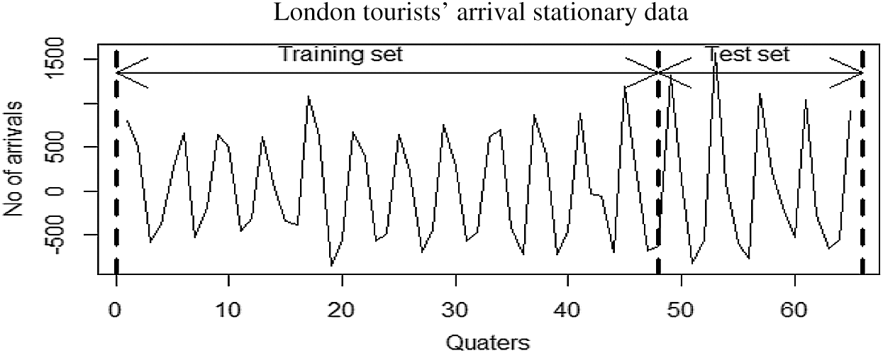
Figure 5: Partition of tourists’ arrival into training and testing part

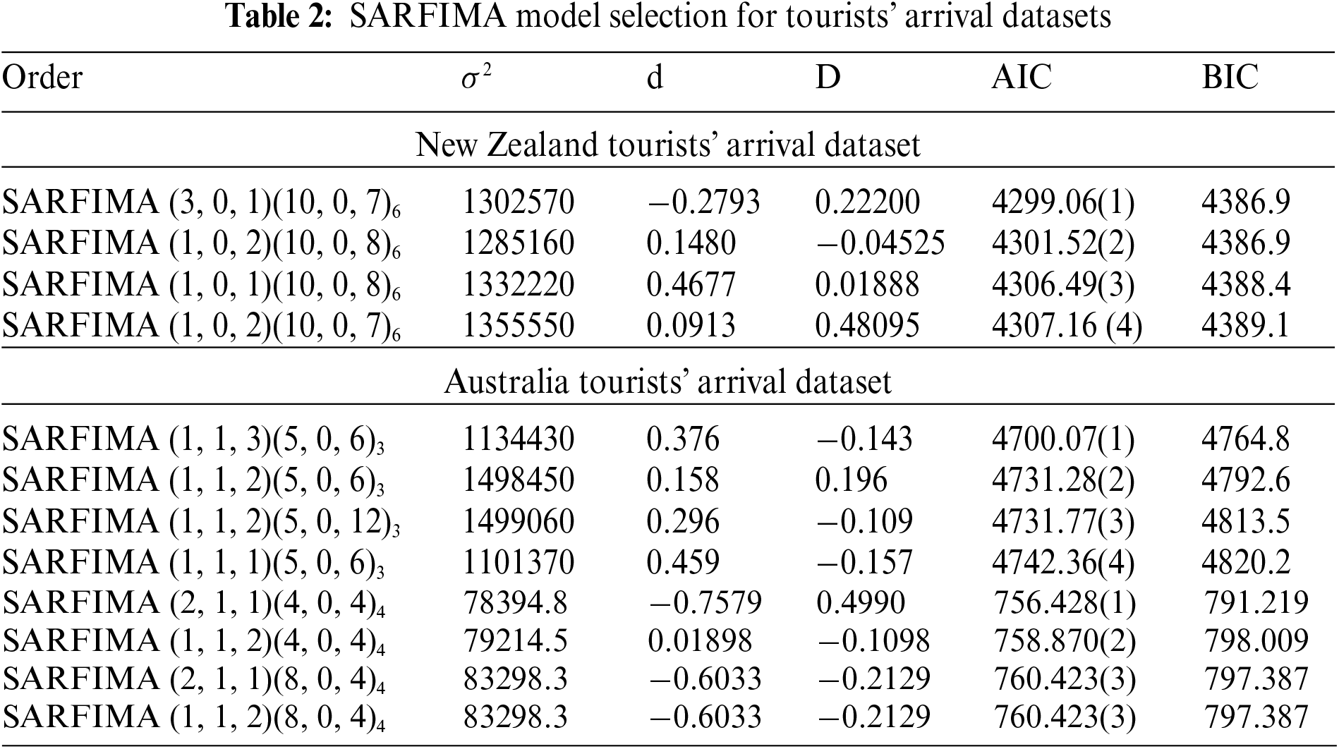
6.1 SARFIMA Model for Tourists’ Arrival Datasets

The fitting of SARFIMA (p,d,q)(P,D,Q)s model on training part of tourists’ arrival datasets requires suitable values for p,q, P and Q. In the case of New Zealand and Australian tourists’ arrival datasets, we take p=1,2,3,4;P=10,11,13;q=1,2 and Q=7,8,9,13,14 on the basis of autocorrelation functions (ACF) and partial autocorrelation function (PACF) values and pattern. Then we take all possible combinations of p,q, P and Q, and fitted 120 SARFIMA models. Analogously, based on ACF and PAF, the suitable values for the London tourist arrival dataset are p=1, q=1,2, P=4,8, Q=4, and s=4. For this dataset, we further estimate SARFIMA models with all possible combinations of p,q, P and Q. After fitting all possible models on each dataset, we have selected models for each dataset based on the minimum values of Akaike Information criteria (AIC) and Bayesian Information Criteria (BIC), keeping in view the values of d and D satisfy the stationary and long memory process condition. Tab. 2 presents these four best-fitted models along with their ranks. The first ranked models have been observed as the most parsimonious models among all SARFIMA models for each dataset.

6.2 Artificial Neural Network Model

To obtain the most accurate ANN model, numerous ANN models were established for the considered datasets using two hidden layers with varying 2 to 30 nodes in the first hidden layer, and 2 to 7 nodes in the second hidden layer. By varying the number of nodes in the first and second hidden layers, 145 models are developed, whereas each model is trained 50 times. Due to the space limitation, the detailed results are not presented here. However, from these models, the best models are selected based on minimum mean squared error (MSE) and root mean squared error (RMSE). Consequently, we obtain ANN(6×2×1), ANN(4×2×1) and ANN(10×2×1) for New Zealand, Australia, and London tourists’ arrival datasets, respectively. The prediction from the best ANN model for each dataset is presented in Fig. 6 for comparison.

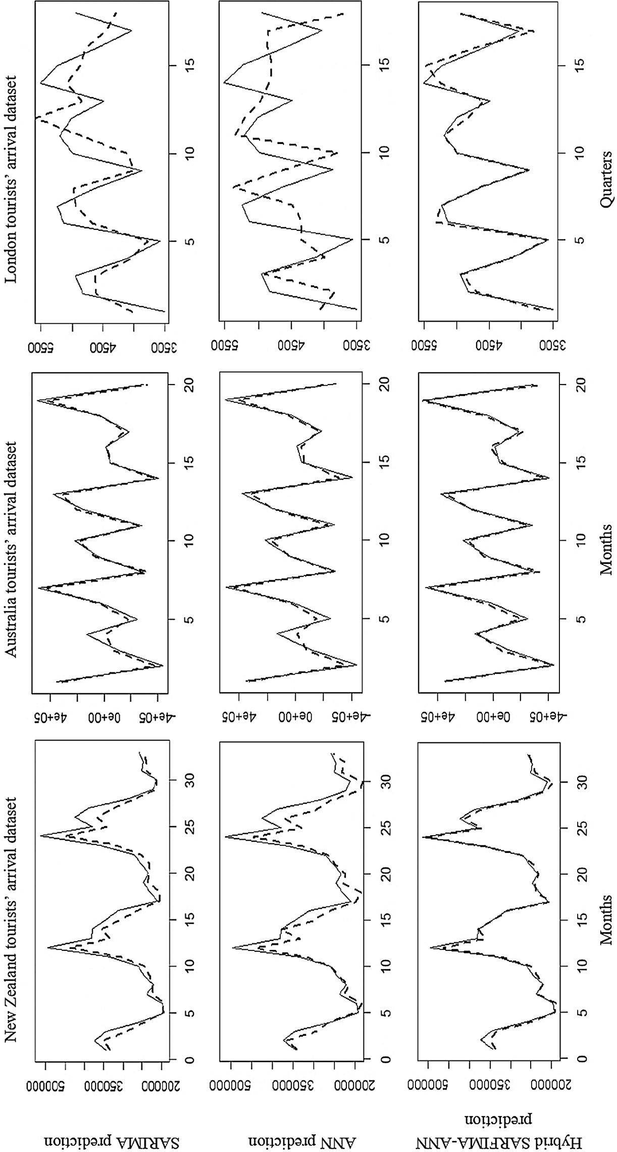
Figure 6: Prediction comparsion among SARFIMA, ANN and hybrid SARFIMA-ANN models (‐‐‐‐ predicted and ––actual values)

6.3 Hybrid SARFIMA-ANN Model

The hybrid algorithm mainly consisted of two steps as discussed earlier. In the first step, a SARFIMA model is fitted to analyze the linear part of the data and in the second step, the residuals from the SARFIMA model are analyzed. Linearity in the residuals is checked using the BDS test as suggested by Broock et al. [41]. In order to perform the BDS test, the following steps are being followed.

i.   Select embedded dimensions (m) value so that the embed time series transforms into m-dimensional vectors by considering each m succeeding point in the series.

ii.   Calculate the correlation coefficient that m-dimensional hyperspace for the proportion of points within a distance ∈ of each other.

UmL(∈)=2L−m+1∑t<m⁡I∈(ytm−ysm).

Here I∈ = {1,if||ytm−ysm||<∈0,otherwise} where ||⋅|| used for supremum norm. BDS test illustrates that if the null hypothesis demonstrates xt series is i.i.d., then Um,I(∈)−Um,L(∈)m with probability one as the sample size tends to infinity and ∈ tends to zero.

iii. Compute BDS test statistic that is defined as

Qm,I=T1/2Um,I(∈)−Um,L(∈)mσm,I(ϵ)

iv. It is a two-tail test. The statement under the null hypothesis will reject when the BDS test statistic is greater than the critical value.

In Tab. 3, the results of the BDS test on residuals from selected models SARFIMA models such as SARFIMA (3, 0, 1)(10, 0, 7)6, SARFIMA (1, 0, 3)(5, 0, 6)6 and SARFIMA (2, 1, 1) (5, 0, 6)4 are presented for tourists’ arrival datasets of New Zealand, Australia, and London.

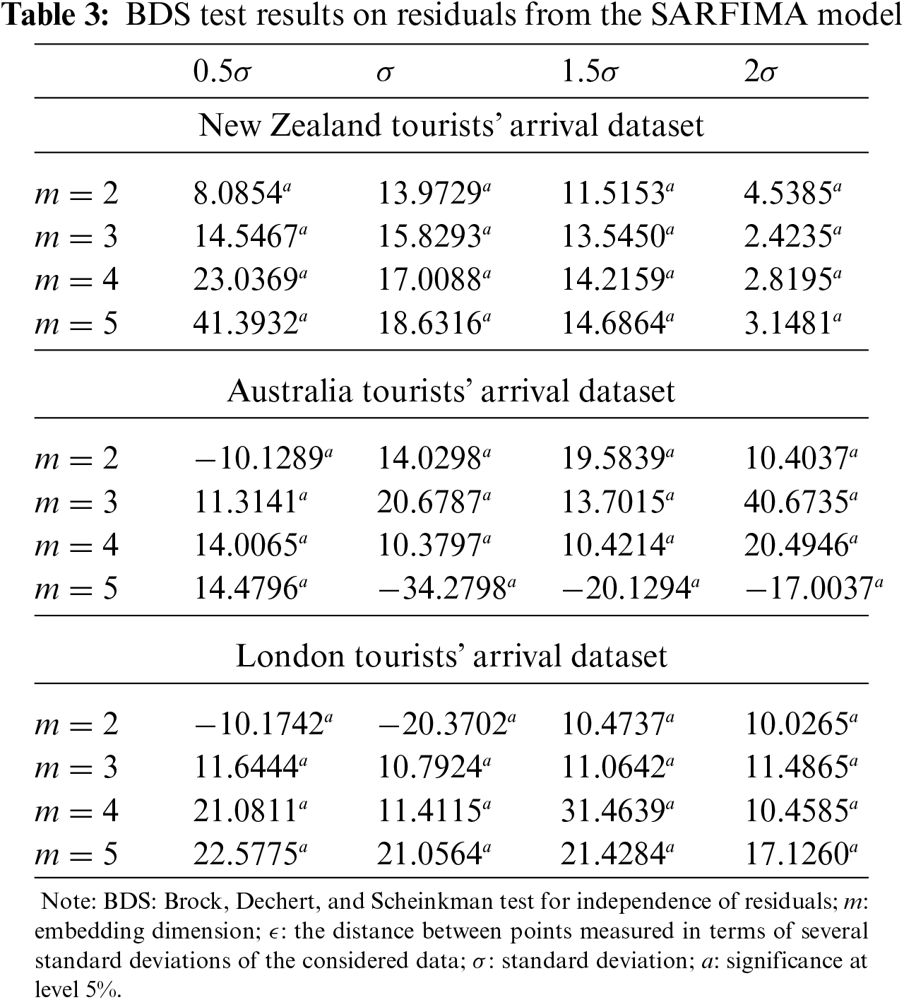
The numerical results of the BDS test, as in Tab. 3, favour rejecting the null hypothesis about the time series linearity at a 5% level of significance. It demonstrates that the errors (residuals) from the best selected SARFIMA models have nonlinear patterns. This indicates that only the linear model (SARFIMA model) is not adequate to model the data well. Therefore, implementation of nonlinear models also requires, such as ANN, to capture the nonlinearity pattern.

We consider the best selected SARFIMA and ANN models, and build the hybrid SARFIMA and ANN models for New Zealand, Australia, and London tourists’ arrival data. Recall Zhang [18] that one can use separate suboptimal models to develop the hybrid method. Following their suggestion, the optimal SARFIMA model is used to model the linear part of the data and the nonlinear patterns fitted by the finalized ANN model. Then the improved prediction is obtained by combining the output of the best fitted SARFIMA and ANN model in the hybrid SARFIMA-ANN model. The performance indicators, that is, MSE and RMSE of the proposed hybrid SARFIMA-ANN and the individuals SARFIMA and ANN models, are presented in Tab. 4. The comparison of the results clearly shows that the proposed hybrid SARFIMA-ANN outperforms than the competing models. Furthermore, the out-of-sample performance of the hybrid and individual models is shown in Fig. 6. We see that the forecasting obtained by the hybrid SARFIMA-ANN model in each dataset is closer to actual than the competing models.

7  Conclusion

Tourism is a rapidly growing industry in most countries and it is demanding more accurate modeling and forecasting of tourists’ arrival data for many purposeful decisions. This, in turn, has grabbed increasing attention to more accurate and advanced forecasting methods. Therefore, the main interest of the study was to establish a possibility for the improvement in the forecast accuracy of tourist arrival using a hybrid modeling approach. Recently, the extension of the SARIMA, which is called the SARFIMA model, has become popular for the linear time series data with long memory processes and periodic patterns. More recently, the ANNs have shown much flexibility in modeling the nonlinear data. Therefore, ANN and SARFIMA can only achieve accurate results in their premises, and generally, none of them is the best model for every forecasting situation. Thus, in this study, a hybrid SARFIMA-ANN approach is established and applied to forecast tourists’ arrival in Australia, New Zealand, and London. This approach is outperformed and produced promising results in the actual situation and produces positive results compared to the two competitors, SARFIMA and ANN. Our results have implications both for theory and application. Theoretically, we developed a hybrid SARFIMA-ANN model. In terms of application, the results of hybrid SARFIMA-ANN provide confidence for policymakers in the search volumes of tourists’ arrival. Consequently, the proposed hybrid SARFIMA-ANN model and the investigation of this study make a good step in improving the forecast accuracy in tourists’ arrival.

Acknowledgement: This research is supported by Artificial Intelligence & Data Analytics Lab (AIDA) CCIS Prince Sultan University, Riyadh 11586 Saudi Arabia. The authors also would like to acknowledge the support of Prince Sultan University for paying the Article Processing Charges (APC) of this publication.

Funding Statement: The authors received no specific funding for this study.

Conflicts of Interest: The authors declare that they have no interest in reporting regarding the present study.

Appendix

A hybrid algorithm based on SARFIMA and Neural network

    Hypothesis: Yt = YtLIN+YtNLIN

    Input: Time series dataset Yt=(yt1,yt1,…,yNt), test to confirm stationarity (adf.test(Yt), pp(Yt), kpss(Yt))

    # Fitting SARIMA model

    Set:  α=aYt, a is a constant, training set size Ntr=N−α, test set size Nts = α, vectors of zeros YtLIN=0[,1:Ntr], YtsLIN^=0[,1:Nts];R=0[,1:Ntr].

      for j in (1:Ntr+Nts) do

                    Yt^(j)=SARFIMA(p,d,q)x(P,D,Q)s,^(Yt,j:j+(Nt−α)−1)

         if j ≤Ntr Then

           R (j) = Yt(j)−Yt^(j)

         else

           Yts^(j)=YtsLIN^=Yt^(j)^

         end if

    end for

    # Fitting ANN model

    Set: YtsNLIN=0[,1:Nts] and Yt=0[, 1:Ntr+Nts]

    for k in (1:Nts) do

YtsNLIN^(k)=ANN(R;p×q×1)

    End for

    Output: Yt = YtsLIN^+YtsNLIN^

This work is licensed under a Creative Commons Attribution 4.0 International License, which permits unrestricted use, distribution, and reproduction in any medium, provided the original work is properly cited.