DOI:10.32604/cmc.2022.024116
| Computers, Materials & Continua DOI:10.32604/cmc.2022.024116 | |
| Article |
Machine Learning-based Stable P2P IPTV Overlay
1Directorate of Information Technology, Sardar Bahadur Khan Women’s University, Quetta, Pakistan
2Department of Computer Science and Information Technology, University of Balochistan, Quetta, Pakistan
*Corresponding Author: Ihsan Ullah. Email: ihsanullah@um.uob.edu.pk
Received: 05 October 2021; Accepted: 30 November 2021
Abstract: Live video streaming is one of the newly emerged services over the Internet that has attracted immense interest of the service providers. Since Internet was not designed for such services during its inception, such a service poses some serious challenges including cost and scalability. Peer-to-Peer (P2P) Internet Protocol Television (IPTV) is an application-level distributed paradigm to offer live video contents. In terms of ease of deployment, it has emerged as a serious alternative to client server, Content Delivery Network (CDN) and IP multicast solutions. Nevertheless, P2P approach has struggled to provide the desired streaming quality due to a number of issues. Stability of peers in a network is one of the major issues among these. Most of the existing approaches address this issue through older-stable principle. This paper first extensively investigates the older-stable principle to observe its validity in different scenarios. It is observed that the older-stable principle does not hold in several of them. Then, it utilizes machine learning approach to predict the stability of peers. This work evaluates the accuracy of several machine learning algorithms over the prediction of stability, where the Gradient Boosting Regressor (GBR) out-performs other algorithms. Finally, this work presents a proof-of-concept simulation to compare the effectiveness of older-stable rule and machine learning-based predictions for the stabilization of the overlay. The results indicate that machine learning-based stability estimation significantly improves the system.
Keywords: P2P IPTV; live video streaming; user behavior; overlay networks; stable peers; machine learning
Live video streaming is a challenging service because it has stringent playback deadlines. Centralized client/server, IP multicast and peer-to-peer (P2P) are major architectures that enable video streaming service. Client/server is a classical approach which allows clients to generate video requests to servers and servers are able to respond to these requests. One major issue of these systems is scalability which requires to enhance the resources at server side to accommodate a surge in user requests, resulting in increased cost. A similar model named as CDN [1] brings some improvements to the classical client/server model to offer video streaming. In CDNs, the source pushes contents to various servers that are distributed purposefully over the Internet. Clients get their contents from nearby servers via any-casting, instead of contacting to source server, which ultimately cuts down the startup delay and reduces the traffic on the network. IP multicast works at the network layer that enables routers to maintain and manage groups. In this approach, one stream can be replicated by a router towards multiple receivers. This approach is an efficient solution but several issues [2] curtailed its deployment over the global scale. However, it is used in smaller domains that are managed by a single administration. On the other hand, P2P strategy works at the application layer [3]. It organizes peers into a virtual network where they not only receive but also transmit the contents. The major advantage of P2P systems over client-server and IP multicast is their easier deployment with low cost.
P2P approach for live streaming has its own issues. One of the major issues of these systems is their reliance on intermittently available nodes which turn the whole system unstable. Numerous approaches have been proposed to overcome this issue, resulting into several systems which can be classified into multiple categories. Such approaches either focus on resilient designs or consider the peer's stability for improvements. The former approach focuses on the overlay network structure and content dissemination strategies which too without stability are not enough as the management overhead is increased as well as the delay.
Concerning stability of peers in existing approaches, it is mostly determined through statistical observation which considers a node to be stable if it is present in the network since long [4–6]. We term this approach as the older-stable principle. This principle is based on general statistical correlation of elapsed time and remaining time of all participating peers in the system. However, users have different choices and habits which influence their viewing patterns. One of the major issues with this approach is the measurement of correlation for sessions of all users together. As a result, strong correlation between elapsed time and remaining time has been observed that assumes long lived peers as stable ones [4]. However, it has been observed that there are different behavior patterns of users during watching television. For instance, a user may leave his/her system on a channel while he/she is busy doing something else, while another user may be joining and leaving channels frequently during browsing mode [7]. This work assesses extensively the older-stable principle through finding the correlation of elapsed time and remaining time in different scenarios. It separates different modes of behaviors and analyzes the correlation in each mode. The results show that this relationship remains different in different scenarios.
Stability of peers can also be predicted through machine learning approach; however, we find very few such efforts in the literature. Therefore, this study also considers machine learning approach for the prediction of stability. To extensively evaluate the accuracy of machine learning algorithms, this work trains and tests several machine learning models. The results show that Gradient Boosting Regressor performs better than other algorithms. Furthermore, to get a comparison of older-stable principle and machine learning based predictions, this work presents a proof-of-concept simulation, and the results indicate that incorporating machine learning-based predictions can significantly improve the performance.
Since P2P networks are networks of users, stability of peers plays a crucial role in the performance of these system. Knowing about stable peers, enables to construct a stream delivery structure in order to improve quality of streaming and provide better user experience. Several types of P2P IPTV overlays exist which can greatly benefit from an accurate estimation of stability. Therefore, this work provides a base line for machine learning based intelligent P2P IPTV overlays.
The contribution highlights of this work are:
▪ Analysis of older-stable principle through finding correlation between elapsed time and remaining time of a session in different scenarios,
▪ Assessment of several machine learning algorithms for the prediction of stability and
▪ Simulation to analyze the effectiveness of machine learning-based stability estimation in a tree-based system.
In the rest of the article, we discuss related work in Section 2. Discussion on analysis of older-stable principle through estimation of correlation and obtained results are presented in Section 3. Section 4 evaluates the efficiency of machine learning algorithms for the prediction of stability. Simulations to compare integration of older-stable principle and machine learning based predictions into a tree-based overlay are given in Section 5. Finally, Sections 6 and 7 present conclusion and future work.
Tang et al. [4] analyze logs of user behavior and observe a positive correlation between the elapsed duration of the current user session and the remaining duration. This motivates them to propose the construction and maintenance of a tree. The tree is built and maintained in such a way that peers with longer presence in the current session are placed near the root of the tree while nodes with shorter presence are placed as leaves. Several other approaches are based on the same older-stable principle. For instance, Wang et al. [5] propose a hybrid push-pull overlay that creates a tree-based backbone called tree-bone from stable nodes and the unstable nodes are connected to the tree-bone. Stream is pushed on the tree-bone while other nodes, out of the tree-bone, function in a mesh network to pull the content. Here, the selection of stable nodes for tree-bone is based on the older-stable principle. Similarly, Tan et al. [6] combine both stability and bandwidth to construct a stable tree where, peer's stability is determined from the online age of the peer.
Tian et al. [7] perform a measurement study of an existing system and observe that nodes’ lifetime follows a Pareto distribution. In their parent selection strategy, they propose to choose older node as a parent node because it is more likely to be a stable one. A two-tiered overlay is presented in [8] where, tier1 consists of stable nodes in the form of a labeled tree. The identification of stable nodes for tier 1 is based on peers’ ages which is like older stable principle. Budhkar et al. [9] propose an overlay management strategy to improve stability of the system. A similar strategy has been used in hybrid P2P-CDN overlay [10]. Fuzzy Logic based Hybrid Overlay (FLHyO) is proposed in [11] that utilizes the fuzzy system to find out the priority of all the peers during overlay construction by considering upload bandwidth, geographical location, age and utilization of a peer. Ma et al. [12] analyze a P2P-CDN based system and propose a peer selection strategy involving machine learning instead of localization. Miguel et al. [13] propose classification of peers based on video chunk contribution. To create partnerships, they restrict each peer to choose partners from high contributing groups as well as low contributing groups to keep the system running. Nonetheless, they do not consider stability of peers in their approach.
On the other hand, prediction of user's current session is proposed in [14] which models the influencing parameters of user behavior through a Bayesian network to predict the length of the current session. Based on the predicted session, they propose to maintain a tree structure that minimizes the impact of abrupt departure of an upstream peer. According to this approach, a peer estimates its own session's length at arrival to the network and schedules a maintenance just before the end of the session. During this stage, it swaps its position with its most stable child while other child nodes are notified to connect to the same or any other stable node. An improvement over the prediction accuracy of the Bayesian network through Support Vector Regressor (SVR) model is presented in [15].
Most of the existing works utilize older-stable principle which considers a peer's age as stability indicator. Furthermore, very few approaches use machine learning to determine the stability which too, do not explore potentially efficient and accurate algorithms. Therefore, this work first extensively evaluates the older-stable principle and then assesses several machine learning algorithms for their accuracy which have not been studied before for this problem.
3 Analysis of Older Stable Principle
To analyze the older stable mechanism, real traces of user activities are required. This study utilizes IPTV traces from Lancaster University [16] where an IPTV service provider (Lancaster living lab) offers video streams both for television sets and PCs installed with P2P clients. These traces contain users’ logs collected over a period of 6 months duration.
Data contain start and stop time of a channel by a user which represent join and departure time. This information can be used to prepare the dataset based on elapsed and remaining time of user where the whole session time is split in one-minute intervals. This provides the data to analyze the correlation between elapsed and remaining time of a user over each minute. An initial analysis of the traces revealed that these traces either contained a large portion of very short sessions or very long sessions spreading over multiple days. Therefore, it is crucial to also analyze the impact of these extreme sessions on overall correlation. To do so, this work calculates the correlation on the whole dataset as well as it separates such sessions from others and analyze them separately. Next, a discussion of different groups of sub-datasets is presented which are separated for analysis.
Users exhibit different behaviors while watching programs. A user is considered to be in surfing mode when he/she is browsing channels and switches channels quickly. In this mode, user checks the current programs of different channels to choose one for watching. Usually, in this mode, a user may hold a channel till to two minutes [17].
A user in viewing mode actually watches the channel and is interested in the content being transmitted. Sessions whose durations remain between the limits of surfing users and idle users are considered in the viewing mode [18]. Additionally, this work also analyzes the correlation over different times of a day as it is evident from the user behavior measurements that behavior changes over daytime.
The presence of very long sessions (days) in dataset demonstrates a very strange phenomenon from which we conclude that these sessions might have resulted from the fact that the television set remained on while the user was not actually watching the channel. Therefore, this study analyzes these sessions separately to understand their correlation. In this work, sessions longer than 4 h are considered to be of an idle user.
This study calculates the Pearson coefficient of correlation as given in Eq. (1). Here,
This sub-section presents the analysis of older-stable principle through finding correlation between elapsed time and remaining time for different behavior groups, as discussed earlier. In addition to existing works, this work studies the impact of daytime on the correlation as well as the impact of each group on the rest of the traces. The Pearson coefficient of correlation, r = 0.71, at p = 0.05 that is statistically significant positive correlation between elapsed time and remaining time for all the traces, ascertaining previous results as presented in [4]. Similarly, for these same combined traces, correlation values for each hour are shown in Fig. 1a.

Figure 1: Correlation of elapsed and remaining time. (a) Group-wise correlation (b) Impact of a group on overall correlation
Here, the correlation remains strong for most part of the day however, it remains quite low during early hours of the day. This shows a little deviation from the existing work when sessions are split in different times. Concerning the analysis of traces from different user groups, traces belonging to surfing behavior show a correlation coefficient of r = 0.07 at p = 0.05 which means that elapsed time has no significant correlation with remaining time. Furthermore, concerning the hourly values, the figure shows again that no significant correlation is found at any hour of the day for surfing behavior.
The value of correlation for viewing users is r = 0.08 at p = 0.05 which is similar to the surfing group. Furthermore, hourly results do not show any strong correlation. On the other hand, the correlation of traces for idle users is r = 0.5 at p = 0.05 which shows that a correlation between elapsed time and remaining time exists. However, it is evident from the hourly result given in the figure, that there is positive as well as negative correlation at different hours of the day. This indeed is an interesting observation which contradicts the older-stable principle. To dig it further, this work combines different behavior groups and presents the results in Fig. 1b. This figure analyzes the effect of each group on overall result. It can be seen that excluding surfing behavior traces has no effect whatsoever on overall result. Moreover, idle behavior has the most impact on the overall result. Therefore, the lack of idle sessions in the traces reduces the value of correlation coefficient.
To understand variations in correlation coefficient during different times of the day, this work analyzes the sessions generated at different times. Fig. 2 presents the histograms of frequency distributions of all the combined sessions at four different timings of the day. It is evident from Fig. 2 that the number of sessions at 04:00, 05:00, and 11:00 are low whereas at 23:00 this number is a lot higher. It means that the number of sessions has also an impact over the correlation coefficient value.

Figure 2: Sessions’ frequency distributions in different day times. (a) Number of sessions at 04:00 (b) Number of sessions at 05:00 (c) Number of sessions at 11:00 (d) Number of sessions at 23:00
Since the older-stable principle is applied to individual users while it is deduced from combined behaviors in existing works, this work also considers the individual case. To perform an analysis of individual behaviors this study extracts traces of two users with most appearances in the system. Figs. 3a and 3b presents the correlations of overall sessions for each of these two users over different times of the day. These results show both very weak positive and negative correlations which means that the general observation of all users together cannot be localized for individual users.

Figure 3: Correlations for individual users. (a) User 1 (b) User 2
To conclude the analysis of older-stable principle, this study observes through extensive investigation that this principle does not always hold. Furthermore, it is dependent on time of the day and overall population of users. The older-stable rule remains intact under the analysis of all the traces of all users together which was established in similar analyses. This study observed that the strong correlation is mainly the result of idle sessions which may be present in a dataset under investigation.
In contrast to older-stable principle, the contextual approach estimates the length of current session of a user from previous sessions as well as contextual information. This section presents an extensive study of the contextual approach to evaluate the efficiency of several machine learning models over the estimation of stability. First, it discusses the machine learning models used in this work and then it presents the methodology adapted in this approach as well as the results.
4.1 Predictive Models for User Behavior
Our goal is to estimate the current session of a user which is a continuous variable therefore it becomes a regression type problem. In the literature, only a Bayesian Network (BN) and Support Vector Regressor (SVR) have been used for the prediction of current session from contextual information [15]. This work includes other machine learning models to get a comparison and enhance the accuracy further. Since, this is a Regression problem, this study applies several Regression models and selects those which produce comparable results. The newer models chosen for this study are K-Nearest Neighbors Regressor (KNNR), Random Forest Regressor (RFR) and Gradient Boosting Regressor (GBR). This work also includes the previously used Bayesian network and SVR models for comparison. First, we discuss all these models.
4.1.1 K-Nearest Neighbor Regression
K Nearest Neighbors Regression is an adapted form of K-Nearest Neighbor (KNN) for continuous variables. KNN is a supervised learning mechanism for the prediction of discrete variables. The core of this technique is the use of nearest neighbors for the estimation of unknown or missing variable. To determine the nearest neighbors, it uses the distance metric such as Euclidean distance from missing point. KNNR estimates the output label by taking an average of the labels of its k-nearest neighbors.
This work uses the Python machine learning library to build the KNNR model. This library provides KNNR that can be configured with different settings according to the nature of the problem. Different parameters are set for this model to get best settings for this problem. A few major parameters and their settings as chosen for this model are described below.
• n neighbors (K):
K is the number of nearest points called neighbors that the algorithm considers estimating a missing point. The value of K has direct impact on the query processing time of a few algorithms such as Ball tree and the KD tree. A larger value of K increases the query time due to two reasons: Firstly, a larger value of K requires to search a bigger part of the neighbors’ space, leading to more time. Secondly, using K > 1 requires queuing of internal results during tree traversal. A value of K = 9 produces better results in this work.
• algorithm: There are different algorithms available that include brute, ball tree, kd tree and auto values. One can set either of these algorithms or otherwise the auto option let the system choose the best one for the problem. This work chooses the latter option.
• P: P specifies the method of computing distance between points. A value of 1 invokes manhattan distance, 2 provides a method equivalent to Euclidean distance and any other random value sets the distance metric as minkowski distance.
Random Forest Regressor combines multiple decision tree classifiers by fitting them on sub-samples of the dataset selected randomly. Further, it averages the results of these classifiers to control over-fitting and enhance accuracy. This work utilizes the model provided by the Python machine learning library [19] to use RFR. This model provides a number of configurable parameters that can be fine-tuned according to the problem. The selected parameters are presented next.
• n estimators: This parameter specifies the number of trees to be used by RFR. This work evaluates the performance of the model with different values and chooses a value of 50 for this parameter as it provides better results.
• criterion: RFR uses this parameter for the measurement of quality of a split. This study selects Mean Squared Error (MSE) as a value of this parameter.
• max depth: This parameter specifies the maximum size of the tree. This work does not impose any such limitation and uses the default value of None for this parameter.
• bootstrap: This parameter is a boolean type which if false, the model uses the entire dataset to construct each tree. This study uses the value true for this parameter.
• max samples: In case the bootstrap value is true, this parameter can be used to limit the size of the sub-samples. This study uses the default value which is None.
4.1.3 Gradient Boosting Regressor
Gradient Boosting is based on AdaBoosting which starts to train a weak learner such as a decision tree through assigning an equal weight to each observation. Once the first tree is evaluated, it changes the weights of observations in such a way that difficult to classify observations get increased weights and easy to classify observations get reduced weights. In the next iteration another tree is grown with new weighted observations. The goal is to improve the predictions of the first tree. At the end of the second iteration, the model is an ensemble of the two trees. This process is continued until a specified number of iterations is achieved.
Gradient Boosting works in similar way by training several models gradually, additively, and sequentially. Gradient Boosting differs from AdaBoost in the identification of limitations of weak learners. In contrast to AdaBoost model, gradient boosting identifies the limitations by using gradients in the loss function such as squared error. This is actually a measure of goodness of fitting model's coefficients to the data. Since this work attempts to predict the session of a user, the loss function would base on the error of the prediction between actual and predicted session.
4.1.4 Support Vector Regressor
Support Vector Regressor (SVR) is a generalization of Support Vector Machine (SVM) for regression problems. SVM models the binary classification problem as convex optimization problem through finding the maximum margins that separate the hyperplane. Support vectors represent the hyperplane. To generalize SVM to SVR, an ε-insensitive region around the function is introduced. This region is termed as ε-tube. This tube attempts to solve the optimization problem for continuous variable through finding a tube that best approximates the continuous variable as well as balancing the complexity of the model and prediction error. In brief, firstly, it finds the flattest tube that contains most of the training instances. Secondly, it solves the convex optimization problem, having a unique solution. The training samples lying outside the tube boundary are contained in support vectors as hyperplane. These are the most influential instances impacting the shape of the tube [20].
This study utilizes the SVR model provided by the Python machine learning library. This model provides several parameters that can be set to fine-tune the model for customized solutions. To describe the configuration of the model used in this work, its parameters are given below.
• Kernel: The Python machine learning library provides several kernel functions such as Linear, Polynomial, Sigmoid, and Radial Basis. Since the Kernel function performs the optimization, its selection is not straightforward. Therefore, this work analyzed the performance of each kernel empirically on the dataset and chose the Radial Basis Function (RBF) kernel provided by [19].
• Gamma: The gamma parameter determines the influence of the spread of training sample. This influence is far for small values while close for large values. This work experiments with different values of this parameter and chooses 0.1 as its value in the developed model.
• Epsilon (ε): Parameter ε is used to control the width of the epsilon-tube. This value influences the number of support vectors which are used to construct the regression function. A greater value of ε means fewer support vectors. Nonetheless, greater values mean more flat estimates. This work experiments with several values and chooses 0.1 as a suitable one.
• C: This is called the regularization parameter which manages the tradeoff between achieving a low training error and a low testing error. It generalizes a model to unseen data. Again, this work chooses through experimentation the value of this parameter which is 100.
The joint distribution of a set of variables having possible mutual causal relationships is represented by a Bayesian network through a directed acyclic graph and conditional probability distributions. The acyclic graph consists of nodes and edges. Nodes represent variables that contain conditional probability distributions while edges represent their causal relationships. The goal of a Beyesian network is to estimate a posterior conditional probability distribution of a target variable after observing the evidence. Each variable in a Bayesian network is conditionally independent from all its child nodes given the states of its parents. This property sometimes significantly reduces the number of parameters that are required to characterize the Joint Probability Distribution (JPD) of variables. For a given Bayesian network, the joint probability distribution over U can be computed as shown in Eq. (2).
Building a Bayesian network model has two parts, namely structure and parameters. The structure of the model places variables in relationships while parameters are set as prior probabilities of each node. Both of them can be built manually or learned from data [21,22]. This work builds the structure manually as well as learns it from data; however, no significant difference in overall results of the two models is observed. Concerning the parameters, they are learned from data.
The methodology this work adapts for contextual approach is depicted in Fig. 4. It starts with the generation of the dataset and ends by the prediction of session duration. The main stages are data generation and preparation into dataset, model building and validation. We discuss these major parts one by one.

Figure 4: Contextual approach for stability estimation
4.2.1 Data Generation and Preparation
The dataset used earlier in correlation analysis is limited in size therefore, this work uses a synthetic dataset. This dataset is generated through a semi-Morkovian model presented in [23]. The total number of instances generated from this model are 462,825. The dataset contains the following major features.
• Join Time Tj: This field shows the time-of-the-day at which a user joins a channel. The time is represented in minutes and its value is from 1 to 1440.
• Departure Time Td: This feature shows again time-of-the-day at which a user quits a channel. The value of departure time has the same range as of join time.
• Session Duration: The time duration in minutes between the join time and departure time is session duration in our dataset. This variable shows the stability of a user and models are tested for accuracy over the estimation of this variable.
• Arrival Rate: Arrival rate or joining rate represents the number of users joining during a particular minute of the day. This field contains value of arrival rates for each minute of the day.
• Departure Rate: Departure rate represents the number of users leaving/quitting a channel during a specific minute of a day. Departure rates for each minute is recorded in this field.
• Population: Just like arrival and departure rates, population is also a collective variable that contains the count of online users at a specific minute of the day.
• Content Type: The model contains three generic kinds of contents which are fiction, sports and real. The dataset records the type of the content being broadcast at each minute.
In feature extraction phase, this work selects variables of interest in light of the work presented in [18]. It calculates the session duration variable from the join time and departure time and selects the variables shown in Fig. 5. Here, session duration is the target variable while other variables have influencing relationships to it.
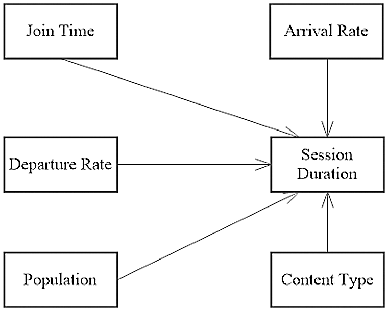
Figure 5: Session duration and related variables
The dataset is split into training set and test set (validation set) using holdout method through the train test split function of Python library [19]. The random state parameter is set to 5, which ensures the same random number sequence generation at each run. The parameter test size is set as 0.3, which randomly splits 30% instances of the actual dataset into test set and remaining in the training set.
4.2.2 Model Building and Validation
This work configures each machine learning model according to the specifications given in the description of models above. Then, it builds every model using the training subset. To test (validate) the model, this work uses the testing set instances. Here, session duration (target variable) is dropped and is let to be predicted by the model for its accuracy assessment during the validation step.
As discussed above each of these models is assessed over the prediction of the session duration. To evaluate the accuracy of each model, this work uses three error calculation techniques namely, Mean Absolute Error (MAE), Mean Squared Error (MSE) and Root Mean Squared Error (RMSE).
● MAE: It is an average of absolute differences between the actual session and the predicted session. The MAE is a linear score which means that all the individual differences are weighted equally in the average. It can be computed through Eq. (3).
where, n denotes the number of records in the data set, y is the actual session, and
● MSE: It calculates the square difference between the model predicted session and the actual session for each point, and then averages these values. MSE can be computed through Eq. (4).
● RMSE: RMSE is calculated in two stages. First, normal mean error is taken. Then, the square root is added to allow the errors ratio to be the same as the targets number. The RMSE can be computed as in Eq. (5).
To compare the results of newly tested models (GBR, KNNR and RFR) to previously used models (BN and SVR), the MAE, MSE and RMSE of all these models are depicted in Fig. 6. It can be easily noted from the figure that GBR, KNNR and RFR produce lower errors than SVR and BN, hence showing more accuracy.
Concerning the MAE, the RFR model produces the lowest error which is 0.83. It means that RFR performs better for outliers. However, being an absolute error, this metric is not considered as a good choice to compare models. Furthermore, the MAE does not assign weights to errors such as, a higher weight to larger errors. Therefore, to compare the accuracy of the models, this study focusses on MSE and RMSE. It can be noted that GBR produces the least MSE and RMSE among all the tested models. Therefore, based on these two metrics, GBR emerges as the best model for this problem.
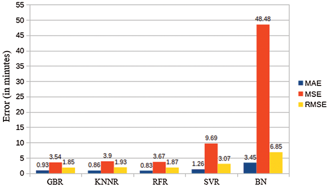
Figure 6: Models’ accuracy
To have a look at individual predictions, a scatter plot of actual vs. predicted values for each of GBR, KNNR, RFR, SVR and BN is shown in Fig. 7. In each plot, the actual sessions are shown on the x-axis and the predicted sessions on the y-axis. In case of an ideally perfect model, the predicted session should be exactly the actual session, therefore the plot will make the slope. Hence, all the over-estimations shall appear above the slope and the underestimations shall appear below the slope. Similarly, more points near the slope with low spread show overall low error.
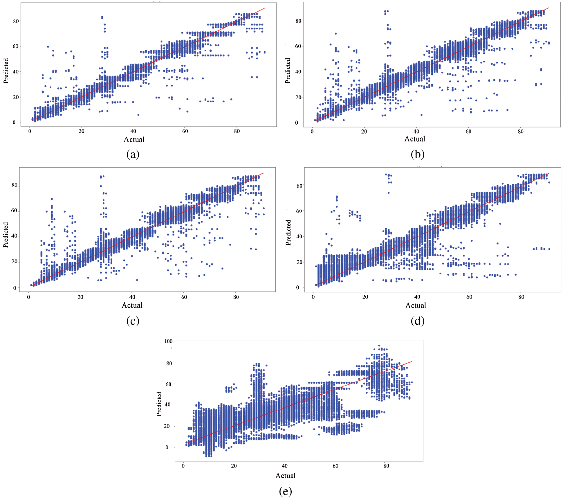
Figure 7: Actual vs. predicted session durations (in minutes). (a) GBR (b) KNR (c) RFR (d) SVR (e) BN
Comparing these plots, affirms the overall performance of each model discussed earlier. Here, all the three newly proposed models show better accuracy then the previous models. Among the three, GBR produces the least spread of points from the slope and therefore shows better accuracy than all the compared models.
5 Stabilization of P2P Overlays
Predictions of machine learning models discussed above can be used to stabilize the P2P overlay. Since there are several stream distribution strategies in P2P IPTV networks, which drives the overlay structure therefore stabilization strategies can be in multiple ways. For instance, a tree can be constructed in such a way that the stable peers are placed near the root while the unstable ones are joined at the leaves. Furthermore, algorithms to maintain a stable tree during the frequent arrivals and departures shall be required. Similarly, in hybrid system, a stable peer may be chosen for the push operation in order to minimize the pull operations.
This work presents a proof-of-concept simulation which considers a single tree system. The data are taken from the logs of one day of the same 10,000 users, used as a dataset in evaluation of machine learning models in three cases of tree construction. In the first case, a tree is built randomly in which peers arrive and leave the system according to their actual join time and departure time. It does not involve any stabilization mechanism. This is termed random in this work. The second case involves the older-stable principle which constructs and maintains the tree based on the elapsed time of the user. It means that the peer present since longer is considered the stable one and is placed higher in the tree. Finally, we construct the tree based on the predicted sessions of the machine learning model. The results of GBR are utilized in this case as GBR was the most accurate model among all tested models.
The simulation starts at minute 1 and simulates the on and off time of each user as given in the dataset. On each minute it checks the join time of each user and if it matches with the current time, it lets the user join an existing peer as a child. Each peer has an outdegree between 1 and 5 which is randomly assigned. Similarly, the departure time of each user is checked on each minute and if it matches the current time, the peer exits. At the same time the number of descendant peers of the departing peer is recorded which shows the impact of departure. The tree is periodically stabilized after every 3 min time according to applied stabilization strategy.
As discussed earlier that intermittent presence of peers is a major issue in P2P IPTV systems, this experiment analyzes the impact of an abrupt departure. The sudden departure of an upstream peer discontinues the stream to all its descendant peers. Therefore, on each departure, this number is counted to show the resilience of a particular tree against such departures.
The simulation is run for each case and the number of impacted peers at every minute is record. Fig. 8a depicts the number of impacted peers in each case. To note the variations in number of online users, the population is also shown in Fig. 8b. It is obvious from Fig. 8a that stabilization based on machine learning predictions minimizes the impact of departures significantly to a negligible level. However, at the other hand, the stabilization based on older-stable rule shows poor performance as compared to other approaches. It might be due to the fact that this dataset does not contain idle sessions therefore correlation-based prediction produces poor results. It also emphasizes the use of a more robust mechanism such as machine learning.

Figure 8: Stabilization comparison. (a) Disruptions (b) Population
This work focusses on the stability of peers in a P2P IPTV architecture. It first extensively analyzed the older-stable principle, the widely used approach for determination of stable nodes. For this purpose, traces of IPTV systems were analyzed for the correlations of elapsed time and remaining time in several scenarios. This analysis revealed that the older stable principle stands true for user sessions when correlation is calculated together. However, in case different behavior groups are separated, this principle does not remain true as very weak, or no correlation is observed. Moreover, in case of individual users, again no correlation was found.
Secondly, machine learning algorithms were evaluated for their accuracy to predict the stability. This study considered GBR, KNNR and RFR and compared their performance with previously used models namely, SVR and Bayesian network. Over the same training and testing data, all these algorithms performed better than SVR and Bayesian network. Furthermore, GBR produced better accuracy among the newly tested models.
Finally, a proof-of-concept simulation was conducted which considered the construction of a tree structure based on three methods. In one method, the tree was randomly constructed without any stability mechanism while in other two methods tree was built and stabilized based on older stable principle and machine learning based predictions. Simulation results revealed that machine learning based stabilization can bring significant improvement to the system.
This work presents a small-scale simulation which only considers a single tree. Therefore, future work needs to consider machine learning-based hybrid topology. Furthermore, concrete experiments on real network are needed to validate the system for implementation in deployed systems. Machine learning can be utilized to include other parameters such as available bandwidth and delay. The same approach can be extended to other user-oriented networks.
Funding Statement: The authors received no specific funding for this study.
Conflicts of Interest: The authors declare that they have no conflicts of interest to report regarding the present study.
1. V. Stocker, G. Smaragdakis, W. Lehr and S. Bauer, “The growing complexity of content delivery networks: Challenges and implications for the internet ecosystem,” Telecommunications Policy, vol. 41, no. 10, pp. 1003–1016, 2017. [Google Scholar]
2. S. Islam, N. Muslim and J. W. Atwood, “A survey on multicasting in software-defined networking,” IEEE Communications Surveys & Tutorials, vol. 20, no. 1, pp. 355–387, 2018. [Google Scholar]
3. M. L. Merani, L. Natali and C. Barcellona, “An IP-TV P2P streaming system that improves the viewing quality and confines the startup delay of regular audience,” Peer-to-Peer Networking and Applications, vol. 9, no. 1, pp. 209–222, 2016. [Google Scholar]
4. Y. Tang, L. Sun, J. -G. Luo and Y. Zhong, “Characterizing user behavior to improve quality of streaming service over P2P networks, in Proc. the 7th Pacific Rim Conf. on Advances in Multimedia Information Processing, Hangzhou, China, pp. 175–184, 2006. [Google Scholar]
5. F. Wang, Y. Xiong and J. Liu, “mTreebone: A collaborative tree-mesh overlay network for multicast video streaming,” IEEE Transactions on Parallel and Distributed Systems, vol. 21, no. 3, pp. 379–392, 2010. [Google Scholar]
6. G. Tan and S. A. Jarvis, “Improving the fault resilience of overlay multicast for media streaming,” IEEE Transactions on Parallel and Distributed Systems, vol. 18, no. 6, pp. 721–734, 2007. [Google Scholar]
7. Y. Tian, D. Wu, G. Sun and K. -W. Ng, “Improving stability for peer-to-peer multicast overlays by active measurements,” Journal of Systems Architecture, vol. 54, no. 1–2, pp. 305–323, 2008. [Google Scholar]
8. F. Wang, J. Liu and Y. Xiong, “On node stability and organization in peer-to-peer video streaming systems,” IEEE Systems Journal, vol. 5, no. 4, pp. 440–450, 2011. [Google Scholar]
9. S. Budhkar and V. Tamarapalli, “An overlay management strategy to improve peer stability in p2p live streaming systems,” in Proc. IEEE Int. Conf. on Advanced Networks and Telecommunications Systems (ANTS), Bangalore, India, pp. 1–6, 2016. [Google Scholar]
10. S. Budhkar and V. Tamarapalli, “An overlay management strategy to improve QoS in cdn-p2p live streaming systems,” Peer-to-Peer Networking and Applications, vol. 13, pp. 190–206, 2020. [Google Scholar]
11. K. Pal, M. C. Govil and M. Ahmed, “FLHyO: Fuzzy logic based hybrid overlay for p2p live video streaming,” Multimedia Tools and Applications, vol. 78, pp. 33679–33702, 2019. [Google Scholar]
12. Z. Ma, S. Roubia, F. Giroire and G. Urvoy-Keller, “When locality is not enough: Boosting peer selection of hybrid cdn-p2p live streaming systems using machine learning,” in Proc. Network Traffic Measurement and Analysis Conf. (TMA), 2021, [Online]. Available: https://tma.ifip.org/2021/wp-content/uploads/sites/10/2021/08/tma2021-paper14.pdf. [Google Scholar]
13. E. C. Miguel, C. M. Silva, F. C. Coelho, I. F. S. Cunha and S. V. A. Campos, “Construction and maintenance of p2p overlays for live streaming,” Multimedia Tools and Applications, vol. 80, pp. 20255–20282, 2021. [Google Scholar]
14. I. Ullah, G. Doyen and D. Gaıti, “Towards user-aware Peer-to-Peer live video streaming systems,” in Proc. IFIP/IEEE Int. Symp. on Integrated Network Management (IM), Ghent Belgium, pp. 920–926, 2013. [Google Scholar]
15. M. Ali, I. Ullah, W. Noor, A. Sajid, A. Basit et al., “Predicting the session of an p2p IPTV user through support vector regression (SVR),” Engineering, Technology & Applied Science Research, vol. 10, no. 4, pp. 6021–6026, 2020. [Google Scholar]
16. Y. Elkhatib, M. Mu and N. Race “Dataset on usage of a live & VOD P2P IPTV service,” in Proc. 14th IEEE Int. Conf. on Peer-to-Peer Computing (P2P), London, UK, IEEE, pp. 1–5, 2014. [Google Scholar]
17. M. Cha, P. Rodriguez, J. Crowcroft, S. Moon and X. Amatriain, “Watching television over an IP network,” in Proc. IMC, Vouliagmeni, Greece, pp. 71–84, 2008. [Google Scholar]
18. I. Ullah, G. Doyen, G. Bonnet and D. Gaiti, “A survey and synthesis of user behavior measurements in video streaming systems,” IEEE Communications Surveys & Tutorials, vol. 14, no. 3, pp. 734–749, 2012. [Google Scholar]
19. F. Pedregosa, G. Varoquaux, A. Gramfort, V. Michel, B. Thirion et al., “Scikit-learn: Machine learning in python,” Journal of Machine Learning Research, vol. 12, pp. 2825–2830, 2011. [Google Scholar]
20. M. Awad and R. Khanna, “Support Vector Regression,” in Efficient Learning Machines, Apress, Berkeley, CA, Ch. 4, pp. 67–80, 2015. [Online]. Available: https://link.springer.com/chapter/10.1007/978-1-4302-5990-9_4. [Google Scholar]
21. T. Talvitie, R. Eggeling and M. Koivisto, “Learning Bayesian networks with local structure, mixed variables, and exact algorithms,” International Journal of Approximate Reasoning, vol. 115, pp. 69–95, 2019. [Google Scholar]
22. L. Azzimonti, G. Corani and M. Zaffalon, “Hierarchical estimation of parameters in Bayesian networks,” Computational Statistics & Data Analysis, vol. 137, pp. 67–91, 2019. [Google Scholar]
23. G. Bonnet, I. Ullah, G. Doyen, L. Fillatre, D. Gaiti et al., “A Semi-markovian individual model of users for P2P video streaming applications,” in Proc. 4th IFIP Int. Conf. on New Technologies,” Mobility and Security (NTMS) IEEE, Paris, France, pp. 1–5, 2011. [Google Scholar]
 | This work is licensed under a Creative Commons Attribution 4.0 International License, which permits unrestricted use, distribution, and reproduction in any medium, provided the original work is properly cited. |