DOI:10.32604/cmc.2022.024309
| Computers, Materials & Continua DOI:10.32604/cmc.2022.024309 | |
| Article |
Machine Learning Based Analysis of Real-Time Geographical of RS Spatio-Temporal Data
Department of Disaster Management, Al-Balqa Applied University, Prince Al-Hussien Bin Abdullah II Academy for Civil Protection, Jordan
*Corresponding Author: Rami Sameer Ahmad Al Kloub. Email: rami.kloub@bau.edu.jo
Received: 13 October 2021; Accepted: 15 November 2021
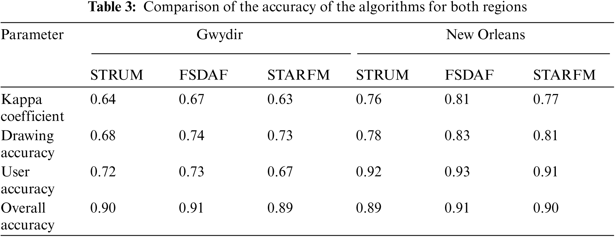
Abstract: Flood disasters can be reliably monitored using remote sensing photos with great spatiotemporal resolution. However, satellite revisit periods and extreme weather limit the use of high spatial resolution images. As a result, this research provides a method for combining Landsat and MODIS pictures to produce high spatiotemporal imagery for flood disaster monitoring. Using the spatial and temporal adaptive reflectance fusion model (STARFM), the spatial and temporal reflectance unmixing model (STRUM), and three prominent algorithms of flexible spatiotemporal data fusion (FSDAF), Landsat fusion images are created by fusing MODIS and Landsat images. Then, to extract flood information, utilize a support vector machine (SVM) to classify the fusion images. Assess the accuracy of your work. Experimental results suggest that the three spatio-temporal fusion algorithms may be used to effectively monitor floods, with FSDAF's fusion results outperforming STARFM and STRUM in both study areas. The overall flood classification accuracy of the three STARFM, STRUM, and FSDAF algorithms in the Gwydir research region is 0.89, 0.90, and 0.91, respectively, with Kappa coefficients of 0.63, 0.64, and 0.67. The flood classification accuracy of the three fusion algorithms in the New Orleans research region is 0.90, 0.89, and 0.91, with Kappa values of 0.77, 0.76, and 0.81, respectively. The spatio-temporal fusion technique can be used to successfully monitor floods, according to this study.
Keywords: Support vector machine; remote sensing; fusion model; geo-spatial analysis; mapping
Floods are one of the world's most common and devastating natural disasters. Due to its rapid, large-scale, and low-cost ground detection capabilities, remote sensing technology has played a significant role in flood monitoring during the last several decades [1]. In general, there are two types of remote sensing monitoring of flood disasters: active and passive [2]. The process of using radars (such as Sentinel-1 and GF-3) to actively produce electromagnetic waves and receive backscattered energy from ground objects is known as active mode. In flood monitoring, remote sensing is becoming increasingly crucial [3–5]. The passive technique (optical remote sensing) is, on the other hand, impacted by clouds and weather, and data collection is difficult when floods occur. Optical remote sensing data, on the other hand, has been widely employed in flood research because of its rich spectrum properties, data diversity, and simplicity of acquisition, processing, and analysis, among other things [6,7]. The use of optical remote sensing data for flood disaster monitoring is the subject of this article.
Currently, remote sensing pictures with limited spatial resolution, such as MODIS, are used to monitor large-scale floods. For example, reference [8] used MODIS pictures to track flood disasters in the Yangtze River's middle reaches over a lengthy period of time. The flood disaster at Dongting Lake was evaluated and studied using MODIS photos, and the loss caused by the flood disaster was assessed in reference [9]. Reference [10] combined the polar orbiting satellite data NPP-VIIRS and the geostationary satellite data GOES-16 ABI to monitor the Houston flood disaster. Although, low spatial resolution images play an important role in large-scale flood monitoring, their low spatial resolution and the existence of a large number of mixed pixels make flood extraction accuracy based on low spatial resolution image data difficult to meet the needs of small area scales. Especially, in the needs of urban flood monitoring. However, medium and high spatial resolution satellites (such as Landsat) are difficult to obtain data after floods due to their revisit cycles and the impact of weather, and their application in flood monitoring is limited [11]. Therefore, how to obtain high-time and high-spatial resolution remote sensing images at the same time is the key to solving this problem. In recent years, the rapid development of remote sensing data fusion technology with different temporal and spatial resolutions has provided a new way to obtain high temporal and spatial resolution images, and made it possible to monitor flood disasters [12].
In the past 10 years, domestic and foreign scholars have achieved a series of results in the field of remote sensing image spatio-temporal fusion [13,14]. The spatial and temporal adaptive reflectance fusion model (STARFM) proposed by [15] is the most widely used fusion algorithm, which weights the time difference, spectral difference and distance difference of MODIS and Landsat images calculation to generate reflectance fusion images. The authors in [16] proposed an enhanced spatial and temporal adaptive reflectance fusion model (ESTARFM) on the basis of STARFM, which effectively solved the problem of STARFM in heterogeneity. The problem that the region cannot be accurately predicted. The authors in [17] proposed a spatial and temporal reflectance unmixing model (STRUM) algorithm based on the decomposition of mixed pixels and applied it to the normalized difference vegetation index (NDVI) remote sensing image fusion, found that the fusion result of STRUM is better than STARFM. The authors in [18] proposed a spatial and temporal data fusion model (STDFA) based on the temporal change characteristics of pixel reflectivity and the texture characteristics of medium-resolution images method, and the spatial and temporal data fusion model (STDFA) is reconstructed on the NDVI data in Jiangning District, Nanjing. The above spatio-temporal fusion algorithm has been widely used in land surface temperature monitoring [19,20], vegetation change monitoring [21], crop growth monitoring [22,23], etc., but few people in China apply it to flood monitoring, and almost no scholar has explored the applicability of different types of spatiotemporal fusion algorithms in flood monitoring. One of the main reasons is that, most spatio-temporal fusion algorithms assume that the reference date and the forecast date have not changed, which cannot accurately monitor sudden changes (such as fires, floods, and landslides). The authors in [24] proposed a flexible spatiotemporal data fusion (FSDAF) for the shortcomings of existing fusion algorithms. The areas where the coverage type has abrupt changes have a more accurate prediction, which also provides a more accurate method for monitoring floods with high-temporal-spatial resolution remote sensing images.
This article aims to solve the problem of difficulty in obtaining high-temporal-resolution images after floods. Three popular and typical spatio-temporal fusion algorithms, STARFM, SRTUM and FSDAF, are selected to merge MODIS and Landsat images to generate high-temporal-resolution images that are missing after the flood. Using support vector machine (SVM) method to extract the flood range of the fusion results, and then analyze the accuracy and applicability of the three spatiotemporal fusion algorithms in flood monitoring.
2 Overview of Study Area and Data Sources
2.1 Overview of the Study Area
In order to evaluate the applicability of the spatiotemporal fusion algorithm in different flood scenarios, this paper selects Gwydir and New Orleans 2 as the study area (Fig. 1). Gwydir is a farm in New South Wales, Australia (E149.28°, S29.08°). The main features include farmland, houses, rivers, bare land and vegetation. A flood that occurred on December 12, 2004 inundated a large amount of farmland and caused huge losses to the locals; New Orleans is a coastal city in Louisiana, USA (W90.01°, N29.97°). The main features are Water bodies, vegetation, wetlands and construction land. Hurricane Katrina that occurred on August 30, 2005 flooded most of the city and became one of the deadliest flood events in the history of the United States.
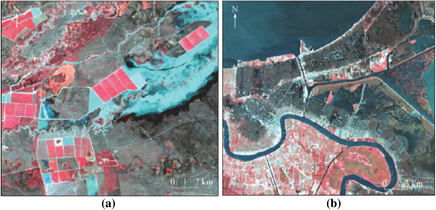
Figure 1: Composite image of the proposed area (a) Gwydir (b) New Orleans
2.2 Data Source and Preprocessing
The research data in this article are MODIS and Landsat images. Among them, the Landsat images of the Gwydir research area were acquired on November 26 and December 12, 2004. December 12 was the flood monitoring day. The Landsat image data size was 800 × 800 pixels; the MODIS image was 500 m spatial resolution per day during the same period. Surface reflectance products (MOD09GA). The Landsat images of the New Orleans research area were acquired on September 7 and October 9, 2005. September 7 was the flood monitoring day. The Landsat image data size was 960 × 960 pixels. Due to the persistence of MODIS daily product data in New Orleans Because of the high cloud coverage, the surface reflectance product (MOD09A1) with a spatial resolution of 500 m over the same period was selected for 8 d.
In addition, the data in the Gwydir research area has been preprocessed [25]. The Landsat image in the New Orleans research area is a Level 1T product, which is a first-class product that has undergone system radiation correction and geometric correction, and only needs to be preprocessed for atmospheric correction. The MODIS 8 d composite product (MOD09GA) is a secondary product that has undergone atmospheric correction and geometric correction. First, you need to use the MRT tool to reproject the MODIS image and convert it to the same UTM projection as Landsat; secondly, resample the MODIS image to Landsat image spatial resolution (30 m); then MODIS and Landsat are geometrically fine-corrected, so that the two images are completely matched, and the error is controlled at 0.5 pixels; finally, the band is adjusted to ensure that the MODIS band and the Landsat band correspond to each other. Fig. 2 is an image of the study area, in which Figs. 2a–2d are Landsat B4 (R), B3 (G), B2 (B) composite images, and Figs. 2e–2h are MODIS B2 (R), B1(G), B4(B) composite image.
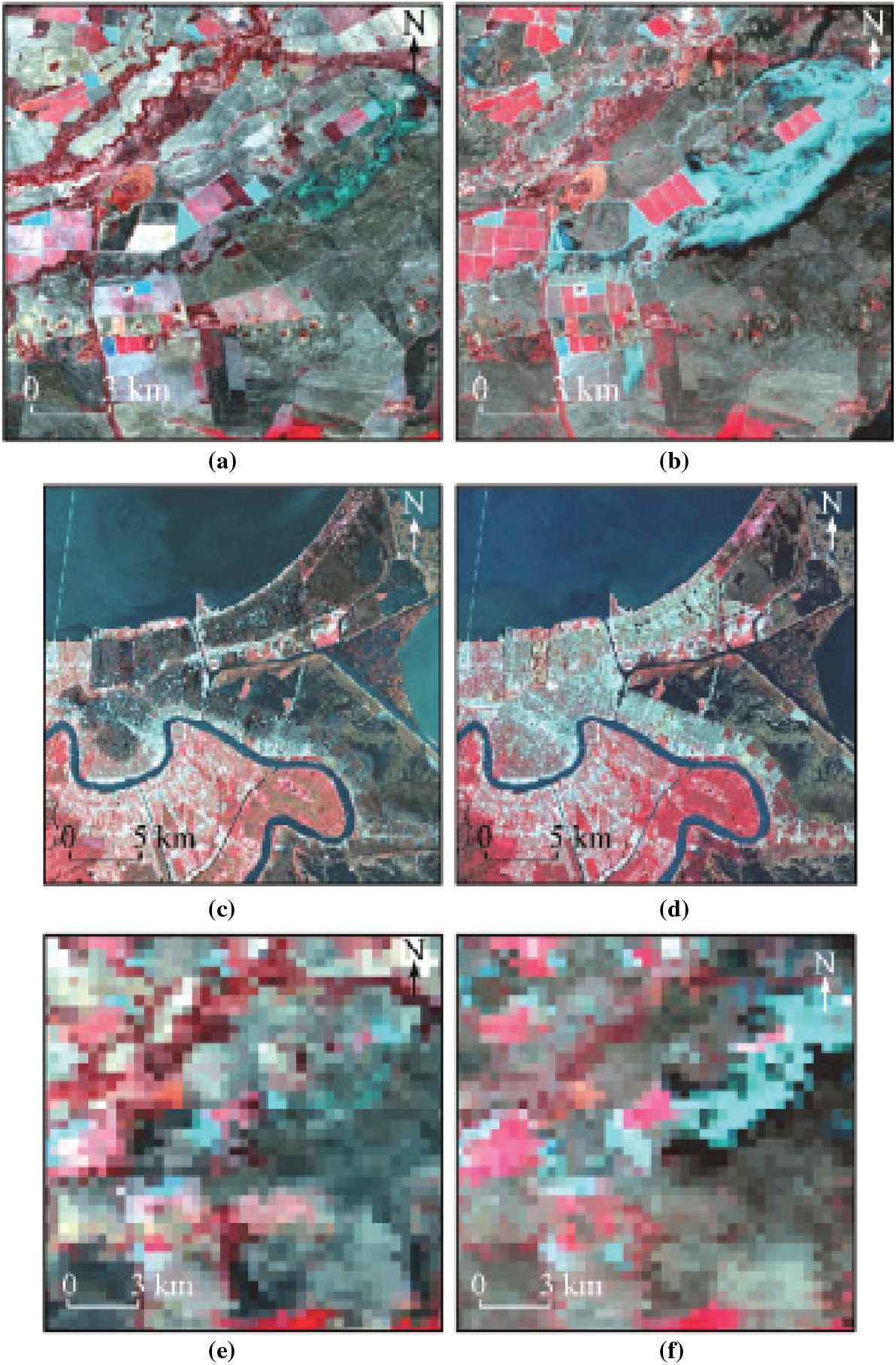
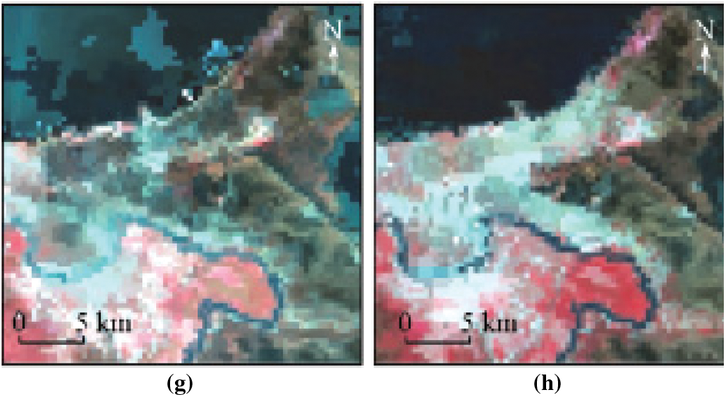
Figure 2: Proposed illustrations of the geographical region (a) 26.11.2004 Gwydir Landsat (b) 12.12.2004 Gwydir Landsat (c) 07.09.2005 New Orleans Landsat (d) 09-10-2005 New Olreans Landsat (e) 26.11.2004 Gwydir MODIS (f) 12.12.2004 Gwydir MODIS (g) 07.09.2005 New Orleans MODIS (h) 09.10.2005 New Orleans MODIS
Three spatio-temporal fusion algorithms, STARFM, STRUM and FSDAF, are used for spatiotemporal fusion of MODIS and Landsat images, and SVM is used to extract floods from the fusion images, and the accuracy of the fusion results and flood extraction results are evaluated. Specific technical processes as in Fig. 3. Among them,
Figure 3: Proposed algorithms flowchart
3.1 Space-Time Fusion Algorithm
STARFM assumes that the Landsat image and MODIS image have consistent correlation on the surface reflectance of the same day, and uses the spectral information of Landsat image and MODIS image and its weighting function to predict the surface reflectance
where i and j are the index positions of Landsat pixels in the moving window; n is the number of similar pixels determined in the moving window;
STRUM predicts the surface reflectance of the image based on the idea of mixed pixel decomposition, and uses Bayes’ theorem to constrain the inaccurate endmember spectrum that may appear in the spectral decomposition process in the process of mixed pixel decomposition. The main steps are:
1) Perform K-means unsupervised classification on
2) Apply the moving window
3) Calculate the reflectance change value
4) Calculate the change value
Wherein
FSDAF combines the method of mixed pixel decomposition and weighting function, and its main steps are:
1) Perform ISODATA unsupervised classification on
2) Estimate the time change
3) Use the category time change obtained in the previous step to calculate the high-resolution image at the
where
4) Use the thin plate spline function to downscale
where
5) According to
where,
6) Use neighboring similar pixels to predict the final result
where
SVM classification method is used for flood extraction. SVM is a non-parametric machine learning method based on statistical theory and the principle of structural risk minimization. It has been widely used in remote sensing image classification. In this paper,
3.3.1 Accuracy Evaluation of Spatiotemporal Fusion Algorithm
In this paper,
3.3.2 Accuracy Assessment of Flood Extraction
The accuracy of flood extraction of three spatiotemporal fusion algorithms is evaluated from two aspects, qualitative and quantitative, using visual discrimination and error matrix. Visual discrimination is to visually compare the flood classification map generated by the fusion of three spatiotemporal fusion algorithms with the standard flood classification map, and intuitively judge the correctness of the water body classification; the error matrix is used to quantitatively evaluate the classification accuracy, and general indicators such as user accuracy and mapping are used. Accuracy, overall accuracy and Kappa coefficient evaluate the accuracy of flood classification. This study is based on the standard flood classification map, which quantitatively evaluates the flood classification map generated by the fusion pixel by pixel, which is closer to the actual situation than the verification method of random placement.
4 Fusion Results and Flood Extraction
4.1 MODIS and Landsat Image Fusion
4.1.1 Results of MODIS and Landsat Image Fusion
Figs. 4 and 5 are the fusion images and verification images of the three spatiotemporal fusion algorithms in the Gwydir and New Orleans study areas, respectively. In order to clearly observe the spatial details of the flooded area, the images of the flooded area in the black box in Figs. 4 and 5 enlarged display.
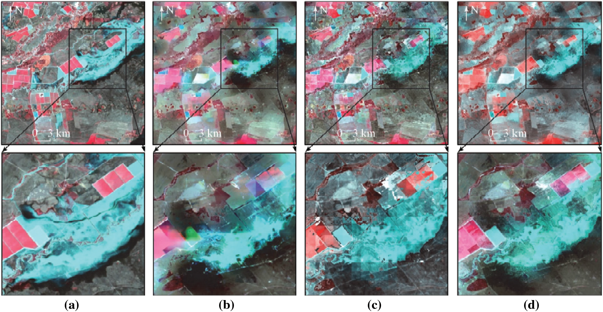
Figure 4: Algorithms comparison of the standard and prediction map of Gwydir (a) verify image (b) STARFM fusion image (c) STRUM fusion image (d) FSDAF fusion image
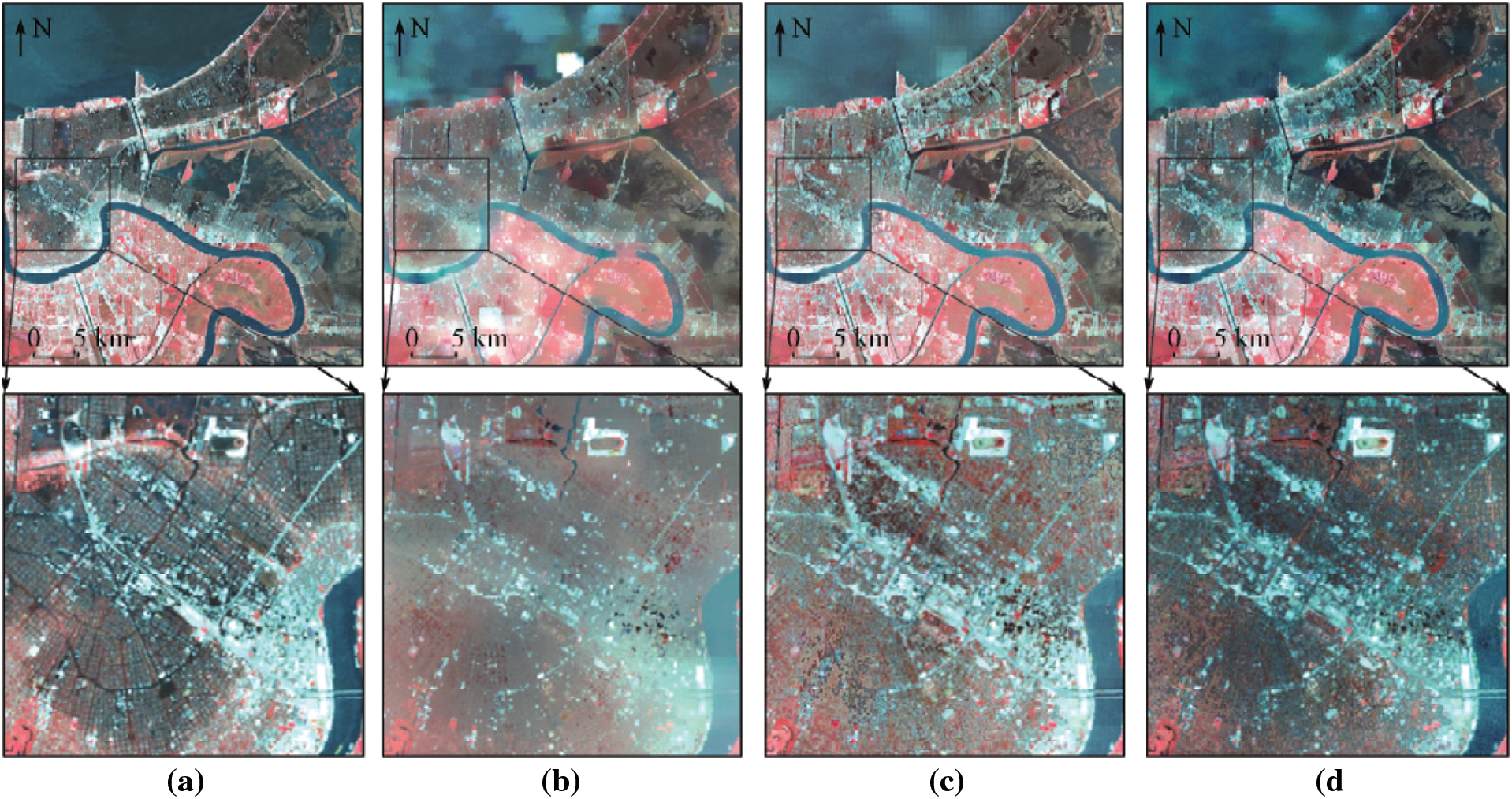
Figure 5: Algorithms comparison of the standard and prediction map of New Orleans (a) verify image (b) STARFM fusion image (c) STRUM fusion image (d) FSDAF fusion image
As in Fig. 4, the comparison of the three algorithms fusion Landsat image and the real image found, and STRUM STARFM algorithm cannot accurately restore the feature information, FSDAF fusion algorithm and compared STARFM STRUM prediction algorithm richer feature information, and differently The boundary of the object type is clearly distinguished; for the flooded area, the STARFM and STRUM algorithms underestimate the area of the water, and the FSDAF algorithm fusion result is closest to the real Landsat image. For the flood edge position, the FSDAF algorithm shows a lower reflectance value than the real Landsat image. In Fig. 5, the fusion results of the three algorithms are relatively close to the true value, but the STARFM algorithm blurs the boundaries of different features, and the STRUM and FSDAF algorithms can restore the feature information more completely. Zooming in on the image of the city center, the STARFM fusion result is worst, as it is impossible to distinguish the boundary between urban buildings and floods. Whereas STRUM is close to the real result, but overestimates the reflectivity value of the flood area. FSDAF has the best prediction effect, which is intuitively the closest to the real image.
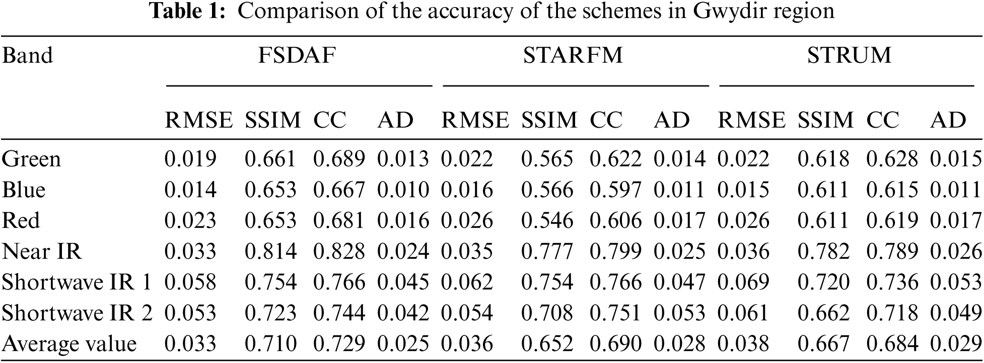
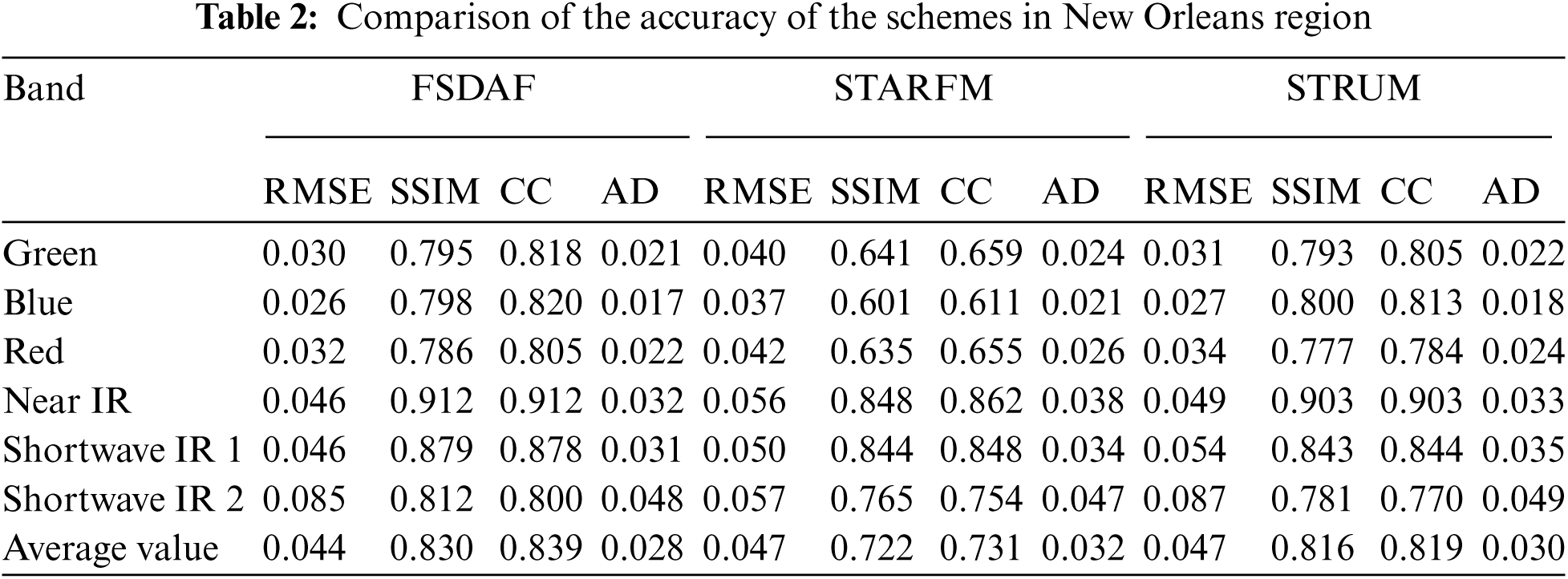
4.1.2 Accuracy Evaluation of Spatio-Temporal Fusion Results
Tabs. 1 and 2 are the accuracy evaluation values of the fusion results of the three spatiotemporal fusion algorithms in the Gwydir and New Orleans study areas, respectively. It can be seen from Tab. 1 that the four index values of the STARFM and STRUM algorithms are similar, the fusion accuracy of the two algorithms is similar, and the accuracy of the FSDAF algorithm is higher than that of the STARFM and STRUM algorithms as a whole. The average CC values of the three algorithms of STARFM, STRUM and FSDAF are 0.690, 0.684, 0.729, and the average values of SSIM are 0.652, 0.667, 0.710, respectively. This shows that the fusion result of the FSDAF algorithm is closer to the real image than the STARFM and STRUM algorithms. In Tab. 2, analyzing the 4 indicators of the 3 algorithms, it can be seen that the STARFM algorithm has the worst accuracy, the STRUM algorithm is better than STARFM, and the FSDAF algorithm is better than STRUM. The average values of RMSE of the three algorithms are 0.032, 0.030 and 0.028, and the average values of CC are 0.731, 0.819 and 0.839, respectively. In addition, the flood has low reflectivity in the near-infrared. The evaluation index parameters of the near-infrared in Tabs. 1 and 2 (CC is 0.799, 0.789, 0.828 and CC is 0.862, 0.903, 0.912) also show that the overall accuracy of the three algorithms is FSDAF algorithm Optimal, STARFM and STRUM algorithms are similar.
4.2 Flood Information Extraction Based on MODIS and Landsat Fusion Images
4.2.1 Extraction of Flood Information from Images Fused
Figs. 6 and 7 are respectively the three spatiotemporal fusion algorithms fused image flood classification map in the Gwydir and New Orleans study areas. In general, the results of (b)-(d) in Fig. 6 are relatively close to (a), but the local differences are more obvious. As Fig. 6 red oval frames illustrated, STARFM algorithm cannot accurately distinguish between water and non-water body, and to overestimate range of the water body, Strum and FSDAF algorithm more accurately capture the boundaries of water bodies. As can be seen in the black block, the three algorithms cannot accurately restore the boundaries of features and underestimate the boundaries of water bodies. In Fig. 7, the three algorithm flood classification maps are relatively close to the real value, and the local differences are small. Intuitively, the extraction results of the three algorithms overestimate the scope of the water body. The red elliptical box in Fig. 7 shows that the STARFM algorithm underestimates the range of the water body, and the extraction results of the STRUM and FSDAF algorithms are consistent with the real image; the black box shows the range of the water overestimated by the STRUM and FSDAF algorithms, and the STARFM algorithm is close to the real image. In general, the FSDAF algorithm has the highest flood classification accuracy in the two study areas, and the STARFM and STRUM algorithms have similar flood classification accuracy.
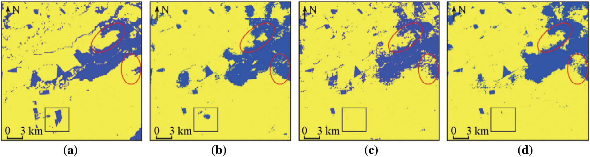
Figure 6: Comparison of the standard and proposed algorithms classification for Gwydire region (a) standard classification (b) STARFM classification (c) STRUM classification (d) FSDAF classification
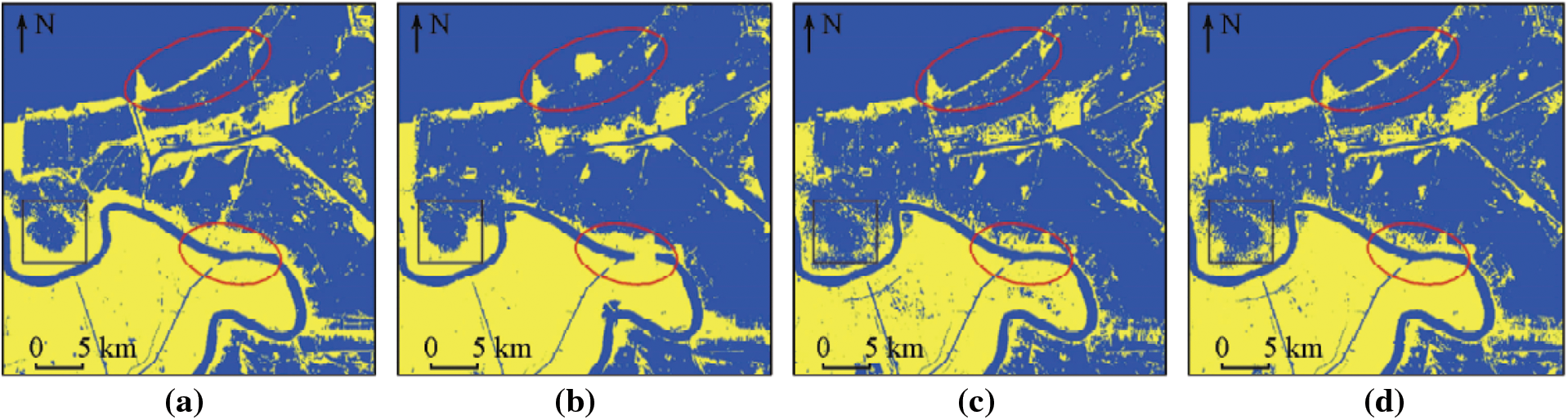
Figure 7: Comparison of the standard and proposed algorithms classification for New Orleans region (a) Standard classification (b) STARFM classification (c) STRUM classification (d) FSDAF classification
4.2.2 Extraction of Flood Extraction Accuracy
Tab. 3 shows the results of flood classification accuracy assessment. It can be seen that the overall accuracy of the three fusion algorithms in the Gwydir and New Orleans research areas is about 0.9, and the range of the water body is more accurately extracted on the whole. But there are inconsistent omissions and misclassifications and errors of the three algorithms. The score rate and the missed score rate in the Gwydir sample area are higher than the New Orleans study area, and the missed score rate and wrong score rate of the FSDAF algorithm are the lowest, and the flood range extraction is closest to the real classification map. In addition, the Kappa coefficients of the three algorithms in the table also show that the FSDAF algorithm is better than the STARFM and STRUM algorithms in flood monitoring [26].
At present, remote sensing spatio-temporal fusion algorithms are generally divided into four categories [27], which are fusion algorithms based on weight function, based on mixed pixel decomposition, based on machine learning, and a mixture of multiple methods. The reasons for choosing the STARFM, STRUM and FSDAF algorithms in this paper are: 1) The three fusion algorithms STARFM, STRUM, and FSDAF are typical algorithms based on weight function, mixed pixel decomposition and hybrid methods, respectively; 2) All three fusion algorithms only need one set of MODIS with Landsat images, the data is easy to obtain and easy to compare and analyze. In addition, two different types of flood events are selected for the purpose of exploring the monitoring capabilities of the spatiotemporal fusion algorithm in different flood scenarios.
The flood prediction results of the three algorithms are compared and analyzed. The overall accuracy of the STARFM, STRUM and FSDAF algorithms in the two sample areas is about 90%, and they can monitor floods well, but the three algorithms have inconsistent omissions and errors. It is divided, and showed the same law in the two study areas. Specifically: FSDAF algorithm has lower error and missing points than STARFM and STRUM algorithms, and the error and missing points of STARFM and STRUM algorithms are similar. Based on the above results and the principle of the algorithm for analysis: 1) The STARFM algorithm assumes that the input image date and prediction date have not changed and the land type has not changed and the MODIS pixels are pure pixels. Its prediction in heterogeneous regions and mutation regions is inaccurate, that is to say, for different features The boundary and the area where the feature type changes cannot be accurately predicted; 2) The STRUM algorithm assumes that the land type has not changed and the mixed pixel decomposition does not consider the variability within the same feature category, and its prediction accuracy is close to that of the STARFM algorithm; 3) The FSDAF algorithm combines STARFM and STARFM. The advantage of the STRUM algorithm, and the introduction of thin-form strip function interpolation for residual distribution. The prediction accuracy of the changed area is higher. The FSDAF algorithm is more suitable for flood monitoring than the STARFM and STRUM algorithms. However, none of the three algorithms can accurately predict small changes in land cover types, especially in areas of heterogeneity.
In addition, the input data of the spatio-temporal fusion algorithm and the flood extraction method affect the final prediction result. First of all, the types of features in the input data have a greater impact on the final results. Specifically, the more types of features in the input data, the small changes in the boundaries of different features cannot be accurately predicted. This is also the fusion accuracy of the three algorithms in Gwydir overall. An important reason for the upper lower than New Orleans. Secondly, the shorter the interval between the input data date and the forecast date, the smaller the change of the features, and the higher the final forecast accuracy. In addition, because the training samples of SVM classification are affected by human subjective factors, the final flood extraction results will have a certain deviation from the actual situation. Other methods such as improved normalized water index can replace SVM for flood range extraction.
In view of the difficulty in obtaining remote sensing images with high temporal and spatial resolution after the flood, it is proposed to fuse MODIS and Landsat images to generate high temporal and spatial resolution images. Taking the Gwydir and New Orleans two areas as the study area, using STARFM, STRUM and FSDAF three spatiotemporal fusion algorithms to fuse MODIS and Landsat images to generate high spatiotemporal resolution images, using SVM to extract the flood range, and combining real Landsat images in the same period for accuracy evaluation. Concluded as follow:
1) The fusion results of the three algorithms are close to the actual images, but the STARFM and STRUM algorithms have poor prediction results in heterogeneous regions. Compared with the STARFM and STRUM algorithms, the FSDAF algorithm is more accurate in restoring the details of the ground features.
2) The overall accuracy of flood extraction of the three algorithms is about 0.9. Compared with the actual Landsat image, it is found that the FSDAF algorithm has lower error and missing points than the STARFM and STRUM algorithms.
3) The three spatio-temporal fusion algorithms can be applied to different flood scenarios and have strong robustness. The FSDAF algorithm can replace the STARFM and STRUM algorithms for accurate flood monitoring with high temporal and spatial resolution.
4) This study applies three spatio-temporal fusion algorithms to flood monitoring, and the FSDAF algorithm has a higher fusion accuracy than STARFM and STRUM algorithms. However, none of the three fusion algorithms can accurately predict small changes in land cover types. The next step is to combine fusion algorithms based on machine learning to improve the prediction accuracy of areas where land types have changed.
Acknowledgement: The author would like to thanks the editors and reviewers for their review and recommendations.
Funding Statement: The author received no specific funding for this study.
Conflicts of Interest: The author declare that he has no conflicts of interest to report regarding the present study.
1. S. Sebastiano, D. Silvana, B. Giorgio, G. Moser, E. Angiati et al., “Information extraction from remote sensing images for flood monitoring and damage evaluation,” Proceedings of the IEEE, vol. 100, no. 10, pp. 2946–2970, 2012. [Google Scholar]
2. F. Zhang, X. L. Zhu and D. S. Liu, “Blending MODIS and landsat images for urban flood mapping,” International Journal of Remote Sensing, vol. 35, no. 9, pp. 3237–3253, 2014. [Google Scholar]
3. L. Yu, M. Sandro, P. Simon and R. Ludwig, “An automatic change detection approach for rapid flood mapping in sentinel-1 SAR data,” International Journal of Applied Earth Observation and Geoinformation, vol. 73, pp. 123–135, 2018. [Google Scholar]
4. C. Marco, P. Ramona, P. Luca, N. Pierdicca, R. Hostache et al., “Sentinel-1 InSAR coherence to detect floodwater in urban areas: Houston and hurricane harvey as a test case,” Remote Sensing, vol. 11, no. 2, pp. 1–21, 2019. [Google Scholar]
5. W. Kang, Y. Xiang, F. Wang, L. Wan and H. You, “Flood detection in gaofen-3 SAR images via fully convolutional networks,” Sensors, vol. 18, no. 9, pp. 1–13, 2018. [Google Scholar]
6. B. Biswa, M. Maurizio and U. Reyne, “Flood inundation mapping of the sparsely gauged large-scale Brahmaputra basin using remote sensing products,” Remote Sensing, vol. 11, no. 5, pp. 1–16, 2019. [Google Scholar]
7. N. T. Son, C. F. Chen and C. R. Chen, “Flood assessment using multi-temporal remotely sensed data in combodia,” Geocarto International, vol. 36, no. 9, pp. 1044–1059, 2019. [Google Scholar]
8. G. Amarnath and A. Rajah, “An evaluation of flood inundation mapping from MODIS and ALOS satellites for Pakistan,” Geomatics, Natural Hazardz and Risk, vol. 7, no. 5, pp. 1526–1537, 2015. [Google Scholar]
9. N. Vichut, K. Kawamura, D. P. Trong, N. V. On, Z. Gong et al., “MODIS-Based investigation of flood areas in southern Cambodia from 2002–2013,” Environments, vol. 6, no. 5, pp. 1–17, 2019. [Google Scholar]
10. M. Goldberg, S. M. Li, S. Goodman, D. Lindsey, B. Sjoberg et al., “Contributions of operational satellites in monitoring the catastrophic floodwaters due to hurricane harvey,” Remote Sensing, vol. 10, no. 8, pp. 1–15, 2018. [Google Scholar]
11. C. Huang, Y. Chen, S. Zhang, L. Li, K. Shi et al., “Surface water mapping from Suomi NPP- VIIRS imagery at 30 m resolution via blending with landsat data,” Remote Sensing, vol. 8, no. 8, pp. 1–18, 2016. [Google Scholar]
12. R. Ghosh, P. K. Gupta, V. Tolpekin and S. K. Srivastav, “An enhanced spatiotemporal fusion method-implications for coal fire monitoring using satellite imagery,” International Journal of Applied Earth Observation and Geoinformation, vol. 88, no. 3, pp. 1188–1196, 2020. [Google Scholar]
13. A. Comber and M. Wulder, “Considering spatiotemporal processes in big data analysis: Insights from remote sensing of land cover and land use,” Transactions in GIS, vol. 23, no. 5, pp. 879–891, 2019. [Google Scholar]
14. A. Radoi and M. Datcu, “Spatio-temporal characterization in satellite image time series,” in IEEE 8th International Workshop on the Analysis of Multitemporal Remote Sensing (Multi-Temp), Annecy, France, pp. 1–6, 2015. [Google Scholar]
15. F. Gao, J. Masek, M. Schwaller and F. Hall, “On the blending of the landsat and MODIS surface reflectance: Predicting daily landsat surface reflectance,” IEEE Transactions on Geoscience and Remote Sensing, vol. 44, no. 8, pp. 2207–2218, 2006. [Google Scholar]
16. X. L. Zhu, J. Chen, F. Gao, X. Chen and J. G. Masek, “An enhanced spatial and temporal adaptive reflectance fusion model for complex heterogeneous regions,” Remote Sensing of Environment, vol. 114, no. 11, pp. 2610–2623, 2010. [Google Scholar]
17. C. M. Gevaert, F. Haro and A. Javier, “A comparison of STARFM and an unmixing-based algorithm for landsat and MODIS data fusion,” Remote Sensing of Environment, vol. 156, no. 8, pp. 34–44, 2015. [Google Scholar]
18. C. H. Fung, M. Wong and P. Chan, “Spatio-temporal data fusion for satellite images using Hopfield neural network,” Remote Sensing, vol. 11, no. 18, pp. 1–14, 2019. [Google Scholar]
19. P. Wu, H. Shen, L. Zhang and F. Gottsche, “Integrated fusion of multi-scale polar-orbiting and geostationary satellite observations for the mapping of high spatial and temporal resolution land surface temperature,” Remote Sensing of Environment, vol. 156, no. 9, pp. 169–181, 2015. [Google Scholar]
20. J. Tang, J. Zeng, L. Zhang, R. Zhang, J. Li et al., “A modified flexible spatiotemporal data fusion model,” Frontiers of Earth Science, vol. 14, pp. 601–614, 2020. [Google Scholar]
21. F. Gao, T. Hilker, X. L. Zhu, M. Anderson, J. Masek et al., “Fusing landsat and MODIS data for vegetation monitoring,” IEEE Geoscience and Remote Sensing Magazine, vol. 3, no. 3, pp. 47–60, 2015. [Google Scholar]
22. M. Usman and J. E. Nichol, “A Spatio-temporal analysis of rainfall and drought monitoring in the tharparker region of Pakistan,” Remote Sensing, vol. 12, no. 3, pp. 1–15, 2020. [Google Scholar]
23. G. N. Vivekananda, R. Swathi and A. Sujith, “Multi-temporal image analysis for LULC classification and change detection,” European Journal of Remote Sensing, vol. 54, no. 2, pp. 189–199, 2021. [Google Scholar]
24. X. L. Zhu, E. H. Helmer, F. Gao, D. Liu, J. Chen et al., “A flexible spatiotemporal method for fusing satellite images with different resolutions,” Remote Sensing of Environment, vol. 172, no. 18, pp. 165–177, 2016. [Google Scholar]
25. I. Emelyanova, T. Mcvicar, T. Van, L. Li and A. Dijk, “Assessing the accuracy of blending landsat-MODIS surface reflectances in two landscapes with contrasting spatial and temporal dynamics: A framework for algorithm selection,” Remote Sensing of Environment, vol. 133, no. 14, pp. 193–209, 2013. [Google Scholar]
26. D. Zhong and F. Zhou, “A prediction smooth method for blending landsat and moderate resolution imagine spectroradiometer images,” Remote Sensing, vol. 10, no. 9, pp. 1–23, 2018. [Google Scholar]
27. X. L. Zhu and F. Y. Cai, “Spatiotemporal fusion of multisource remote sensing data: Literature survey, taxonomy, principles, applications, and future directions,” Remote Sensing, vol. 10, no. 4, pp. 1–15, 2018. [Google Scholar]
 | This work is licensed under a Creative Commons Attribution 4.0 International License, which permits unrestricted use, distribution, and reproduction in any medium, provided the original work is properly cited. |