Computers, Materials & Continua DOI:10.32604/cmc.2022.024722
Article

Estimator-Based GPS Attitude and Angular Velocity Determination

Dah-Jing Jwo*

Department of Communications, Navigation and Control Engineering, National Taiwan Ocean University, Keelung, 202301, Taiwan
*Corresponding Author: Dah-Jing Jwo. Email: djjwo@mail.ntou.edu.tw
Received: 28 October 2021; Accepted: 09 December 2021

Abstract: In this paper, the estimator-based Global Positioning System (GPS) attitude and angular velocity determination is presented. Outputs of the attitude estimator include the attitude angles and attitude rates or body angular velocities, depending on the design of estimator. Traditionally as a position, velocity and time sensor, the GPS also offers a free attitude-determination interferometer. GPS research and applications to the field of attitude determination using carrier phase or Doppler measurement has been extensively conducted. The raw attitude solution using the interferometry technique based on the least-squares approach is inherently noisy. The estimator such as the Kalman filter (KF) or extended Kalman filter (EKF) can be incorporated into the GPS interferometer, potentially providing several advantages, such as accuracy improvement, reliability enhancement, and real-time characteristics. Three estimator-based approaches are investigated for performance comparison, including (1) KF with measurement involving attitude angles only; (2) EKF with measurements based on attitude angles only; (3) EKF with measurements involving both attitude angles and body angular rates. The assistance from body mounted gyroscopes, if available, can be utilized as the measurements for further performance improvement, especially useful for the case of signal-challenged environment, such as the GPS outages. Modeling of the dynamic process involving the body angular rates and derivation of the related algorithm will be presented. Simulation results for various estimator-based approaches are conducted; performance comparison is presented for the case of GPS outages.

Keywords: Global positioning system (GPS); extended Kalman filter; attitude determination; angular velocity

1  Introduction

Global Positioning System (GPS) [1–5] has traditionally been a position, velocity and time sensor using the code observations. Code and carrier phase observations are two types of observations that can be extracted from the GPS signals. Due to its higher accuracy and precision compared to code observations, carrier phase observations have been used to achieve very high accuracy of estimated position. It provides relative positioning in centimeter level and has been widely applied to surveying, precision approach and automatic landing, and attitude determination [6–10]. Although carrier phase observable can be very accurately measured, it is not possible to use pure carrier phase observable for absolute positioning due to inherent integer cycle ambiguity [9,10]. Positioning or attitude determination using GPS does not have the error accumulation, which happens in the inertial navigation system (INS) [11,12].

Since the carrier phase observables contain much smaller measurement noise than code observables, much effort has been given to develop a technique to utilize the carrier phase observables. By measuring the phase of the GPS carrier relative to the carrier phase at a reference site, single, double, and triple differences can be used to determine the vector between the reference (designated master) and slave antennas and subsequently solve for the attitude determination solutions. If two antennas are attached to a vehicle, a baseline vector defined as a vector from master antenna to the other antenna can be determined using relative positioning techniques. Very accurate relative position estimate will be available if the integer ambiguities are resolved. The attitude of a vehicle can be precisely determined using GPS carrier phase measurements from more than two antennas attached to the vehicle.

Two main issues, real-time integer ambiguity resolution techniques and attitude determination, are to be resolved to determine the vehicle attitude when applying GPS carrier phase double differences. There have been many efforts on real time GPS attitude determination problem. Most of the investigations have been on the real-time integer ambiguity resolution techniques and attitude determination from the baseline vectors. Some investigators utilize certain constrain factors such as baseline length or known geometry to resolve integer ambiguity in real-time manner [13,14].

This paper presents estimator-based GPS attitude and angular velocity determination. Since the attitude solution using the interferometry technique [15–18] based on the least-squares method is inherently noisy, the estimator-based method [12,19–23] using the Kalman filter or the extended Kalman filter possesses good potential for performance enhancement. Measurement for the EKF can be provided by the GPS interferometer, and possibly by the gyroscopes, depending on the availability. The assistance from body mounted gyroscopes, if available, can be utilized as the measurements for further performance improvement. This design provides the opportunity when body angular rates information from other sensor such as the gyroscopes is available for better resistance to the signal-challenged environment, such as the GPS outages.

The remainder of this paper is organized as follows. Preliminary background on GPS attitude and angular velocity determination is reviewed in Section 2. In Section 3, attitude and angular velocity estimator using the extended Kalman filter is briefly introduced. In Section 4, illustrative examples are presented to evaluation of the effectiveness of the proposed algorithm. Conclusions are given in Section 5.

2  GPS Attitude and Angular Velocity Determination

Carrier phase observables in GPS include sum of range, an unknown integer ambiguity and some ranging errors, expressed as:

pseudorangeobservable:ρ=r+c⋅(dt−dT)+dion+dtrop+vρ(1)

carrierphaseobservable:ϕ=r+c⋅(dt−dT)+λ⋅N−dion+dtrop+vϕ(2)

where the parameters are defined as r: true range between a satellite and receiver; c: speed of light; dt: offset of the satellite clock from GPS time; dT: offset of the receiver clock from GPS time; dion: ionospheric correction; dtrop: tropospheric correction; λ: carrier phase wavelength; N: carrier phase integer ambiguity; vρ, vϕ: measurement noises of code and carrier phases.

GPS interferometry has been firstly used in precise static relative positioning, and thereafter in kinematic positioning. By using carrier phase observables, the relative positioning is obtained in centimeter level provided that the integer ambiguity is resolved. In the beginning of 1990s, Van Grass et al. [15] conducted research on the GPS to the field of aircraft attitude determination using carrier phase was developed. In their work, the receiver-satellite double difference observation was employed.

The receiver-satellite double differenced observable is formed by a linear combination of four observations:

∇Δ(∙)12ij={(∙)2j−(∙)2i}−{(∙)1j−(∙)1i}(3)

where ‘∙‘ could represent either Φ, r, or N, and the following operators are defined

Δ(∙)=(∙)receiver_2−(∙)receiver_1: between-receiver differencing operator;

∇(∙)=(∙)satellite_j−(∙)satellite_i: between-satellites differencing operator.

Double differenced observable eliminates or greatly reduces the satellite and receiver timing errors. The observation equation between two receivers and two satellites by combining phase data from master (denoted as ‘1’) and slave (denoted as ‘2’) receivers to satellites i and j can be written as

∇Δϕ12ij=∇Δr12ij+λ∇ΔN12ij−∇Δdion+∇Δdtrop+v(4)

For a short baseline, e.g., less than one meter between two antennas, ionospheric and tropospheric parameters become negligible. The resulting double-difference phase equation when ignoring atmospheric, satellite ephemeris, and residual clock errors is given by

∇Δϕ12ij=∇Δr12ij+λ∇ΔN12ij+v(5)

Attitude is defined by the rotation transformation that relates a coordinate system fixed in space to a coordinate system fixed in the body (body frame). The space coordinate system is typically defined to be a local level NED (north-east-down) frame. The baseline vector is defined as the vector between the antennas designated master and one of the slave antennas. The carrier phase differential GPS based on interferometer principles can solve for the antenna vector. The approach is based on the difference in the GPS carrier phase received at two or more nearby antennas connected to a rigid body. Multiple antenna vectors from an antenna array can be used to calculate the vehicle attitude. In general, to determine the three-dimensional attitude, three non-collinear antennas simultaneously receiving signals from two satellites are the minimum requirement. Referring to the configuration as in Fig. 1, when using the carrier phase signal from satellite i, the between-receiver single differenced observable is a linear combination of two phase observables received by two antennas:

Δϕi=ϕ1i−ϕ2i=b⋅ei+λΔNi(6)

Similarly, the single differenced observable received for the same antennas from satellite j is

Δϕj=ϕ1j−ϕ2j=b⋅ej+λΔNj(7)

where b is the baseline vector formed by two antennas, and e represents the line-of-sight unit vector from antennas to satellites. The receiver-satellite double difference is obtained by taking two independent single differences:

∇Δϕ12ij=Δϕi−Δϕj=b⋅(ei−ej)+λ(ΔNi−ΔNj)=b⋅(ei−ej)+λ∇ΔN12ij(8)

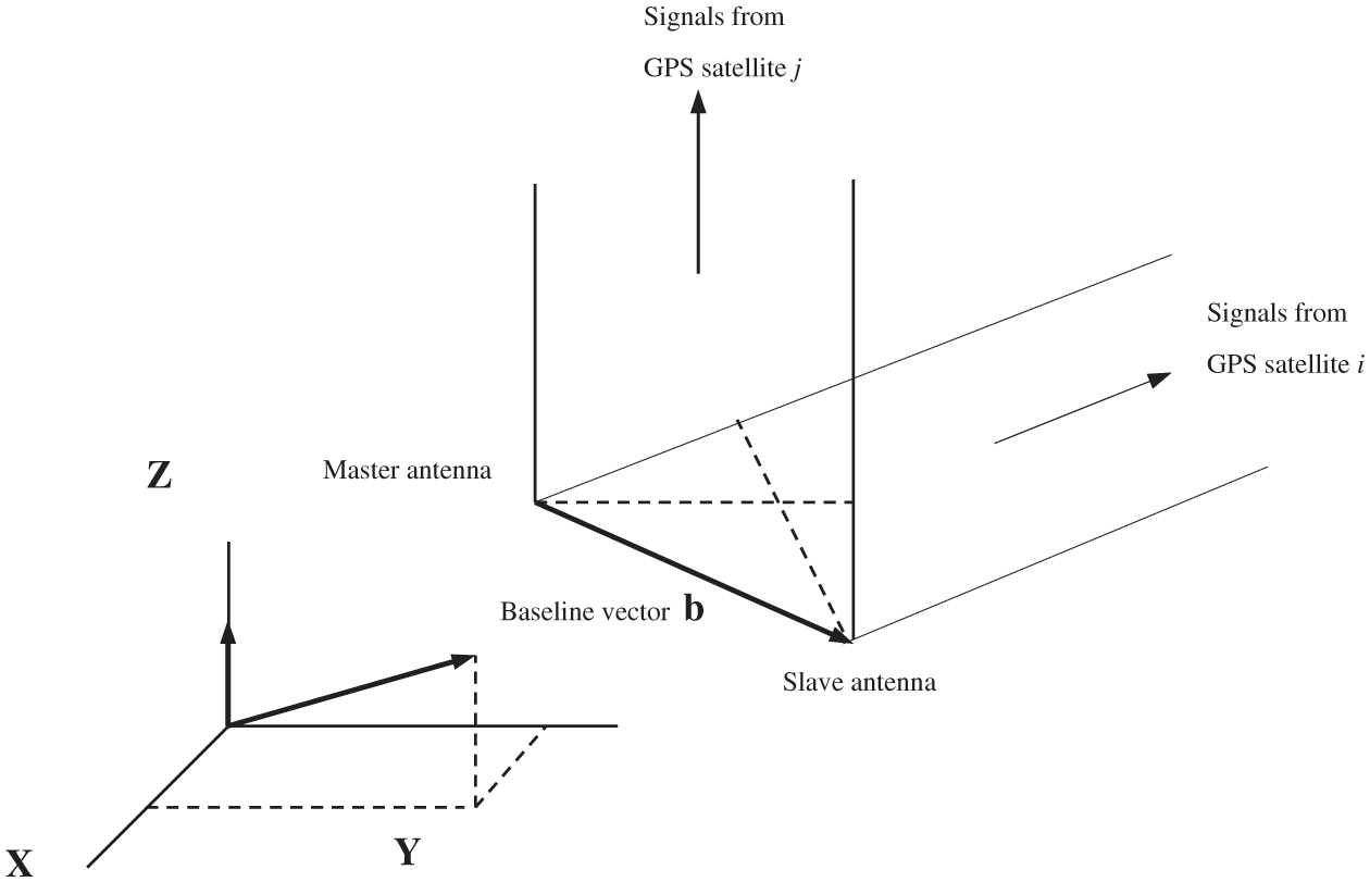
Figure 1: Receiver-satellite double differences [15]

Based on Eq. (8), signals received from (n+1) satellites by one GPS interferometer provide n independent double differences:

[∇ΔΦ1212∇ΔΦ1213⋮∇ΔΦ121n]=[(e1−e2)T(e1−e3)T⋮(e1−en)T][bxbybz]+[λ∇ΔN1212λ∇ΔN1213⋮λ∇ΔN121n](9)

When the integer ambiguity is known, the range-equivalent of Eq. (9) is

[∇Δr1212∇Δr1213⋮∇Δr121n]=[(e1−e2)T(e1−e3)T⋮(e1−en)T][bxbybz](10)

which can be expressed in matrix form ∇Δr=Eb.

There have been many methods proposed for the integer ambiguity resolution, typically including ambiguity function, antenna exchange/swap, baseline rotation methods. The residuals are the differences between the actual double difference measurements and those predicted based on the least-squares solution for b=[bxbybz]T, the approximate interferometer coordinates, and the known satellite coordinates. The accuracy of the attitude measurement depends on the baseline to noise ratio, and is also a function of antenna placement and GPS satellite geometry.

There are several methods available for solving vehicle attitudes, typically including Euler angle method and quaternion method [12,21]. The rotation transformation matrix that relates the NED and body frames provides the information for finding the vehicle attitude:

Rn2b=[CψCθSψCθ−Sθ−SψCϕ+CψSθSϕCψCϕ+SψSθSϕCθSϕSψCϕ+CψSθSϕ−CψSϕ+SψSθCϕCθCϕ](11)

where the subscripts n and b represent the local and body frames, respectively, and we defined the notations S≡sin and C≡cos. Since Rn2b is an orthonormal matrix, its inverse is easily founded to be

Rb2n=Rn2b−1=Rn2bT(12)

Finally, the vehicle attitude can be obtained through the relation:

θ=sin−1(−R13);ϕ=sin−1(R23cos⁡θ);ψ=sin−1(R12cos⁡θ)(13)

To perform the calculation of attitude determination, the antennas should be set up as nonzero and are on the non-collinear vector. Once the baseline vector is determined, estimation of the coordinate frame transformation R^b2n can be achieved and subsequently the transformation matrix from body to local frame can be estimated through the calculation

R^b2n=B^n(Bb)−1, where B^n=[b^1n,b^2n,b^1n×b^2n] and Bb=[b1b,b2b,b1b×b2b].

Once the Euler attitude angle rates are available, the body angular velocity can be found

[pqr]=[10−sin⁡(θ)0cos⁡(ϕ)sin⁡(ϕ)cos⁡(θ)0−sin⁡(ϕ)cos⁡(ϕ)cos⁡(θ)][ϕ˙θ˙ψ˙](14)

However, the attitude angle rate directly obtained from the difference of attitude angles, Θ=[ϕθψ]T between epochs k and k−1 with time interval Δt:

Θ˙=Θk−Θk−1Δt(15)

is usually corrupted and too noisy. Utilization of the Kalman type of filters provides resolves some of the problem.

3  Attitude and Angular Velocity Estimator Using the Extended Kalman Filter

The EKF has been successfully applied in the GPS receiver position/velocity determination, and the integrated GPS/INS navigation system design. In this paper, the KF and EKF will be employed as the estimator for attitude, attitude rates, and body angular velocities to enhance the accuracy and reliability of the attitude solution.

3.1 Implementation of the KF and EKF as the State Estimator

Consider a dynamical system whose state is described by a linear, vector differential equation. The process model and measurement model are represented as

xk+1=ϕkxk+wk,wk∼N(0,Qk)

zk=Hkxk+vk,vk∼N(0,Rk)

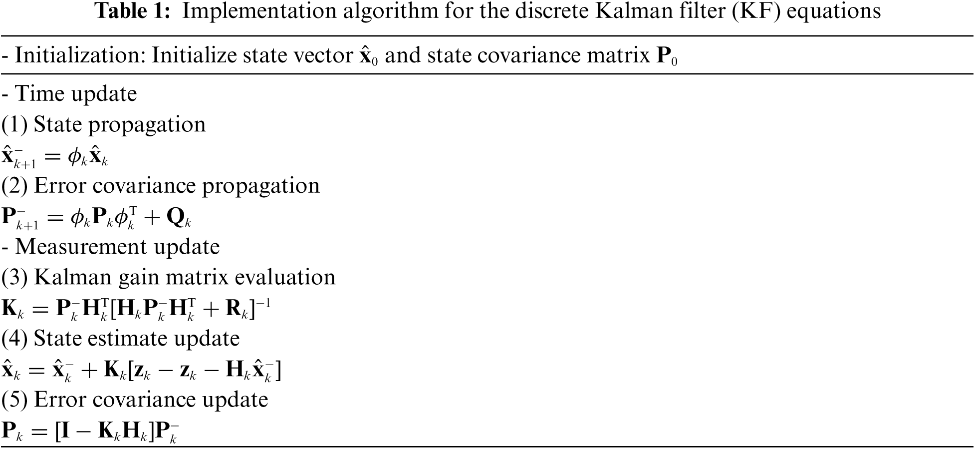
The Kalman filter equations are summarized in Tab. 1.

Consider a dynamical system whose state is described by a nonlinear, vector difference equation. Assuming the process to be estimated and the associated measurement relationship may be written in the form:

xk+1=f(xk,k)+wk(16a)

zk=h(xk,k)+vk(16b)

where the state vector xk∈ℜn, process noise vector wk∈ℜn, measurement vector zk∈ℜm, and measurement noise vector vk∈ℜm. The vectors wk and vk are zero mean Gaussian white sequences having zero cross-correlation with each other:

E[wkwiT]=Qkδik,E[vkviT]=Rkδik,E[wkviT]=0

where Qk is the process noise covariance matrix, Rk is the measurement noise covariance matrix. The symbol δik stands for the Kronecker delta function:

δik={1,i=k0,i≠k

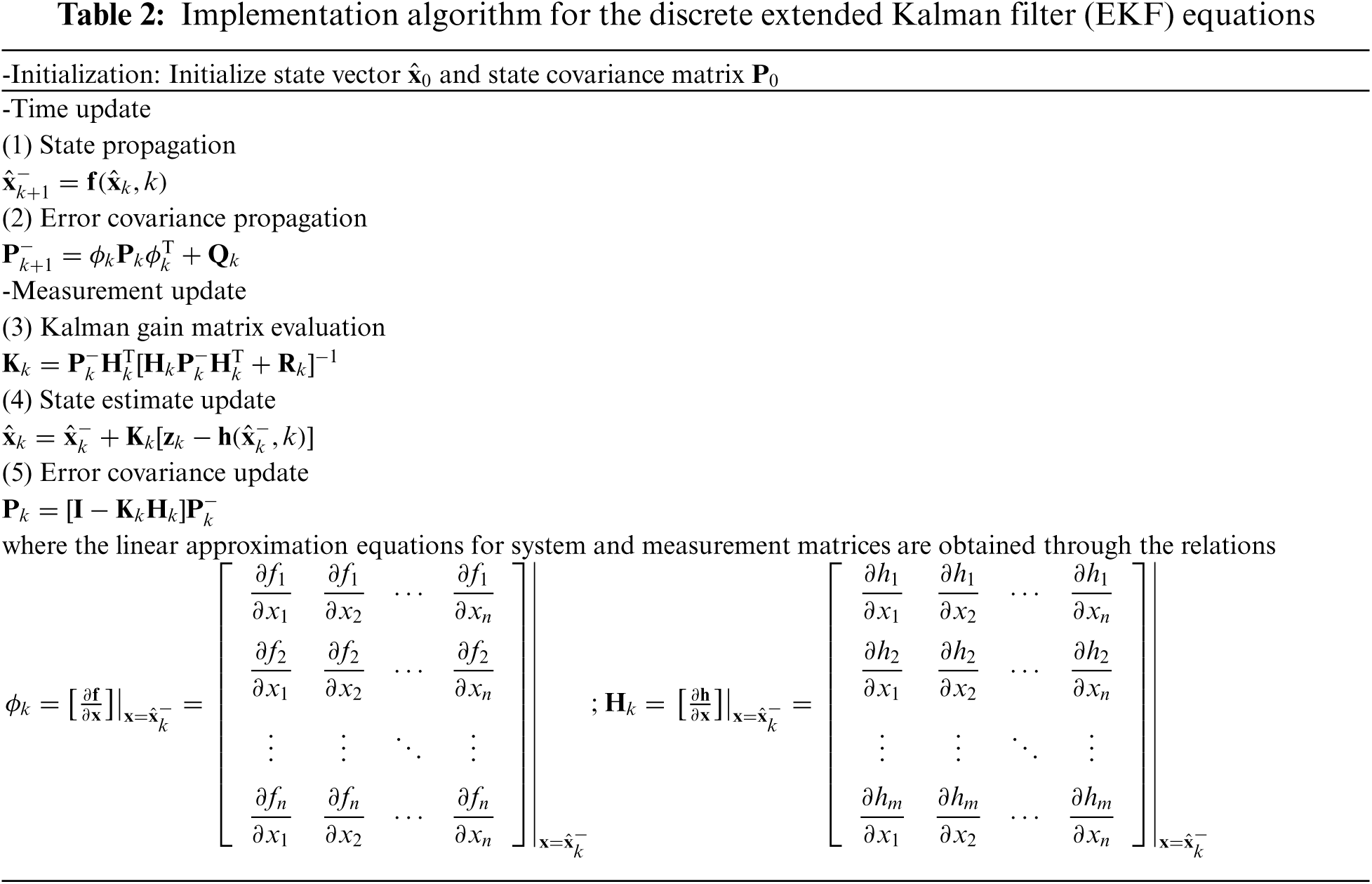
Without external aiding such as an inertial sensor to provide a reference trajectory, the process dynamics represent the total observer dynamics, as shown in Fig. 2. Implementation algorithm for the discrete EKF equations is provided in Tab. 2.

3.2 Modeling of Attitude Dynamics

The appropriate description of the dynamic process model depends on the type of dynamics encountered in a given application.

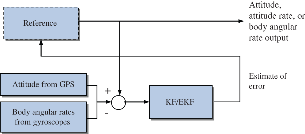
Figure 2: Attitude and angular velocity estimator as a special case of the feedback complementary filter using KF or EKF

3.2.1 Linear System Model Using the KF as the Estimator

A three-state filter model involving the state vector x=Θ=[ϕθψ]T is suitable for a stationary receiver where the attitude states are described as the random walk. This model is equivalent to the P (Position) model in GPS positioning. If the observer is moving nearly constant angular rate, the model corresponding to the double integrator will be more suitable. When the velocity cannot reasonably be modeled as constant, then acceleration states can be added.

(1)   CAV (constant angular velocity) model for the KF

For a low to medium dynamic receiver, a six-state filter model, here referred to as the ‘constant angular velocity’ model, or ‘CAV’ model is employed. The model contains 3 attitude angles and 3 attitude rates, x=[ϕθψϕ˙θ˙ψ˙]T. This model is similar to the PV (Position-Velocity) model in GPS navigation or CV (constant velocity) model in radar tracking. Consider the second-order model, Θ¨=uΘ(t), where Θ=[ϕθψ]T and the noise vector uΘ˙=[uϕuθuψ]T, namely, ϕ¨=uϕ; θ¨=uθ;ψ¨=uψ, we have

ddt[Θ3×1Θ˙3×1]=[03×3I3×303×303×3][Θ3×1Θ˙3×1]+[03×1uΘ](17)

In addition to a pure random walk, an alternative model using the body angular acceleration for the process model can be described as

ϕ¨=−1τϕϕ˙+uϕ,θ¨=−1τθθ˙+uθ,ψ¨=−1τψψ˙+uψ(18)

This model is reasonable since accelerations may not be always constant, but are correlated over short time intervals. Based on Eq. (18), the dynamic process model is given by

ddt[ϕθψϕ˙θ˙ψ˙]=[000100000010000001000−1/τϕ000000−1/τθ000000−1/τψ][ϕθψϕ˙θ˙ψ˙]+[000uϕuθuψ](19)

Furthermore, they can also be modeled as the Gauss-Markov process:

ϕ¨=−βϕ˙+2σ2βuϕ;θ¨=−βθ˙+2σ2βuθ;ψ¨=−βψ˙+2σ2βuψ(20)

(2)   CAA (constant angular acceleration) model for the KF

For a high dynamic receiver, a nine-state filter model, here referred to as the ‘constant angular acceleration (CAA)’ model, with x=[ϕθψϕ˙θ˙ψ˙ϕ¨θ¨ψ¨]T can be considered. The third-order model has the form Θ⃛=uΘ(t), where Θ=[ϕθψ]T and the noise vector uΘ¨=[uϕuθuψ]T. Selecting the state vector that contains the Euler attitude angles, Θ, the attitude rate, Θ˙, and the angular acceleration, Θ¨. This model is similar to the PVA (Position-Velocity-Acceleration) model in GPS positioning or CA (constant acceleration) model in radar tracking.

Selecting the state vector x≡[Θ3×1TΘ˙3×1TΘ¨3×1T]T, the CAA filter model is given by

ddt[Θ3×1Θ˙3×1Θ¨3×1]=[03×3I3×303×303×303×3I3×303×303×303×3][Θ3×1Θ˙3×1Θ¨3×1]+[03×103×1uΘ](21)

or

ddt[ϕθψϕ˙θ˙ψ˙ϕ¨θ¨ψ¨]=[000100000000010000000001000000000100000000010000000001000000−1/τϕ¨000000000−1/τθ¨000000000−1/τψ¨][ϕθψϕ˙θ˙ψ˙ϕ¨θ¨ψ¨]+[000000uϕuθuψ](22)

3.2.2 Nonlinear System Model Using the EKF as the Estimator

If the body angular velocity information is required, an alternative dynamic model can be applied such that the body angular velocity (p, q, r) estimate can be provided directly via the filter. This design provides a convenient way when the system is assisted by the body mounted rate gyroscopes, which is especially useful in case the GPS attitude information is not available.

(1)   CAV model for the EKF

The state vector is composed of 6 states: x=[ϕθψpqr]T. The attitude rates and the body angular velocity are related by

ϕ˙=p+qsin(ϕ)tan(θ)+rcos⁡(ϕ)tan⁡(θ)

θ˙=qcos⁡(ϕ)−rsin⁡(ϕ)

ψ˙=qsin(ϕ)sec(θ)+rcos⁡(ϕ)sec⁡(θ)

The above system of equations can be written in matrix form

[ϕ˙θ˙ψ˙]=[1sin⁡(ϕ)tan⁡(θ)cos⁡(ϕ)tan⁡(θ)0cos⁡(ϕ)−sin⁡(ϕ)0sin⁡(ϕ)sec⁡(θ)cos⁡(ϕ)sec⁡(θ)][pqr](23)

By combining the dynamic models of the body angular velocities: p˙=up; q˙=uq;r˙=ur, we have the following dynamic process model

ddt[ϕθψpqr]=[0001sin(ϕ)tan(θ)cos⁡(ϕ)tan⁡(θ)0000cos⁡(ϕ)−sin⁡(ϕ)0000sin⁡(ϕ)sec⁡(θ)cos⁡(ϕ)sec⁡(θ)000000000000000000][ϕθψpqr]+[000upuqur](24)

One of the alternative models for the dynamic of body angular rate is given by: p˙=−1τpp+up; q˙=−1τqq+uq; r˙=−1τrr+ur. In such case, we have

ddt[ϕθψpqr]=[0001sin(ϕ)tan(θ)cos⁡(ϕ)tan⁡(θ)0000cos⁡(ϕ)−sin⁡(ϕ)0000sin⁡(ϕ)sec⁡(θ)cos⁡(ϕ)sec⁡(θ)000−1/τp000000−1/τq000000−1/τr][ϕθψpqr]+[000upuqur](25)

Similarly, the Gauss-Markov can also be employed for the case of: p˙=−βpp+2σp2βpup; q˙=−βqq+2σq2βquq; r˙=−βrr+2σr2βrur.

The Jacobian matrix F=∂f∂x can be derived to be

F=[qtan(θ)cos(ϕ)−rtan(θ)sin(ϕ)qsin(ϕ)sec2(θ)+rcos(ϕ)sec2(θ)01sin(ϕ)tan(θ)cos⁡(ϕ)tan⁡(θ)−qsin⁡(ϕ)−rcos⁡(ϕ)001cos⁡(ϕ)−sin⁡(ϕ)qcos(ϕ)sec(θ)−rsin(ϕ)sec(θ)sec(θ)tan(θ)[qsin(ϕ)+rcos⁡(ϕ)]00sin⁡(ϕ)sec⁡(θ)cos⁡(ϕ)sec⁡(θ)000000000000000000](26)

and the corresponding discrete-time model is given by ϕk=exp⁡(F⋅Δt).

(2)   CAA model for the EKF

The state vector for the CAA model involves 9 states: x=[ϕθψpqrp˙q˙r˙]T, where the models for angular accelerations can be represented as: p¨=up; q¨=uq; r¨=ur, yielding the dynamic model

ddt[ϕθψpqrp˙q˙r˙]=[0001sin(ϕ)tan(θ)cos⁡(ϕ)tan⁡(θ)0000000cos⁡(ϕ)−sin⁡(ϕ)0000000sin⁡(ϕ)sec⁡(θ)cos⁡(ϕ)sec⁡(θ)000000000100000000010000000001000000000000000000000000000][ϕθψpqrp˙q˙r˙]+[000000upuqur](27)

Similarly, the alternative model that can be considered is given by p¨=−1τpp˙+up; q¨=−1τqq˙+uq; r¨=−1τrr˙+ur, leading to the process model:

ddt[ϕθψpqrp˙q˙r˙]=[0001sin(ϕ)tan(θ)cos⁡(ϕ)tan⁡(θ)0000000cos⁡(ϕ)−sin⁡(ϕ)0000000sin⁡(ϕ)sec⁡(θ)cos⁡(ϕ)sec⁡(θ)000000000100000000010000000001000000−1/τp˙000000000−1/τq˙000000000−1/τr˙][ϕθψpqrp˙q˙r˙]+[000000upuqur](28)

As mentioned, the Gauss-Markov process can also be employed when necessary:

p¨=−βpp˙+2σp2βpup;q¨=−βqq˙+2σq2βquq;r¨=−βrr˙+2σr2βrur

4  Illustrative Examples

Simulation was conducted for evaluating the estimation performance of GPS-based attitude and angular velocity determination. Computer codes were developed using the Matlab® software with assistance from the commercial software Satellite Navigation (SatNav) Toolbox by GPSoft LLC [24] employed for generation of the GPS satellite orbits/positions and thereafter, the satellite pseudorange, and carrier phase observables, required for simulation. The attitude dynamics for simulation is as follows:

p=π15sin⁡(π60t);q=π20cos⁡(π150t);r=3π100cos⁡(π300t)+0.03

with initial attitude ϕ0=θ0=ψ0=0. The attitude rates and body angular velocities in the simulation are shown in Fig. 3.

Three algorithms are involved for testing their performance, including

(1)   KF with measurement involving attitude angles only;

(2)   the first algorithm using EKF (herein referred to as the EKF1), for which the measurements involving attitude angles only;

(3)   the second algorithm using EKF (herein referred to as the EKF2), for which the measurements involving both attitude angles and body angular rates (possibly from gyroscopes).

Tab. 3 summarizes the three architectures employed in this paper for comparison evaluation.

To avoid the filter divergence, it should be noticed that setting the process noise PSD to zero is not acceptable, since it can be very detrimental to the filtering performance, especially if the vehicle is maneuvering rapidly. As a result, when the system reaches steady-state condition, the steady-state gain won't become zero and, subsequently, the filter is able to follow the time-varying attitude dynamics. A small value is admissible in practical design. However, one still needs to find the appropriate values that meet the requirement. The CAV model is employed for investigation since the dynamic for the illustrative is moderate. For the CAV model, the noise strengths for the process and measurement models are selected as:

Qk=[0.1I3×303×303×30.01I3×3];Rk=[I3×303×303×31e−5I3×3]

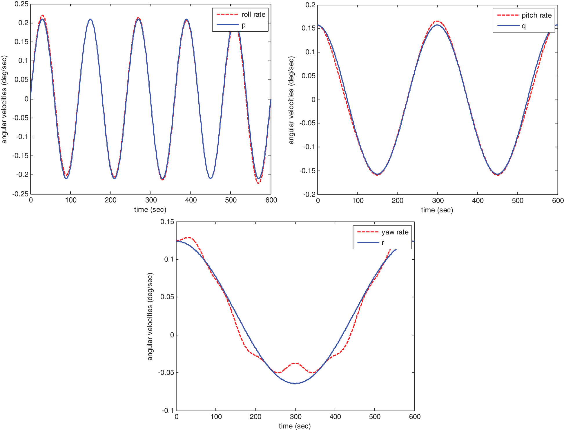
Figure 3: Attitude rates and body angular velocities in the simulation

Simulation results are shown in Figs. 4–8. Figs. 4 and 5 show the performance comparison for KF and EKF1 where Fig. 4 presents estimate of attitude angles without signal outage and Fig. 5 presents those with signal outage. It can be seen that the results from both architectures are equivalent for the case that no outage occurs while the results from EKF1 provides improved performance in some situation, but not so noticeably.

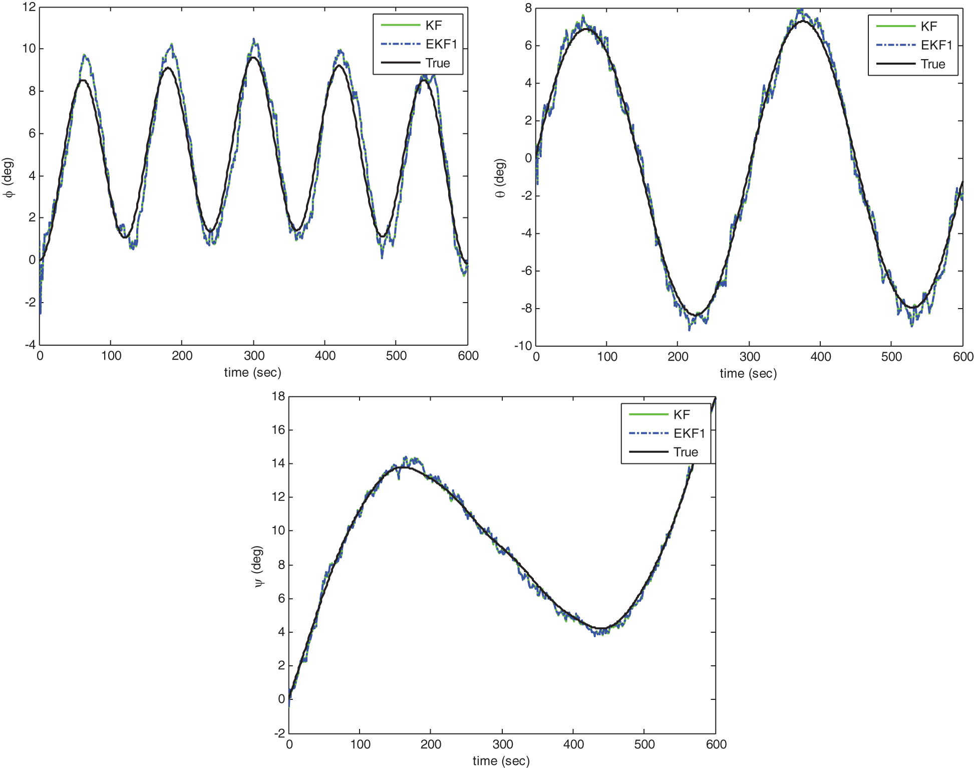
Figure 4: Estimate of attitude angles without signal outage: KF vs. EKF1

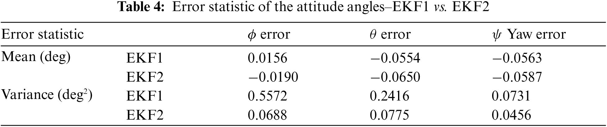
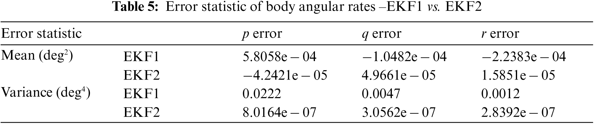
Figs. 6 and 7 show the performance comparison for EKF1 and EKF2 without signal outage. Fig. 6 shows estimate of attitude angles and Fig. 7 provides estimate of body angular rates. It can be seen that the EKF2 approach, with more measurement information available, outperforms the EKF1 approach noticeably. Notice that the solution provided by EKF2 is very close to the true states for the high quality rate gyros. Comparison of the error statistics for EKF1 and EKF2 regarding the attitude angles and body angular rates, respectively, are summarized in Tabs. 4 and 5, respectively. In addition, Fig. 8 shows estimate of attitude angles with signal outage for KF and EKF2. The assistance from body mounted gyroscopes, if available, can be utilized as the measurements for further performance improvement, especially useful for the case of GPS outages. Incorporation of the information of angular velocities into the EKF as the measurement not only achieves better accuracy but also catches the attitude dynamics well.

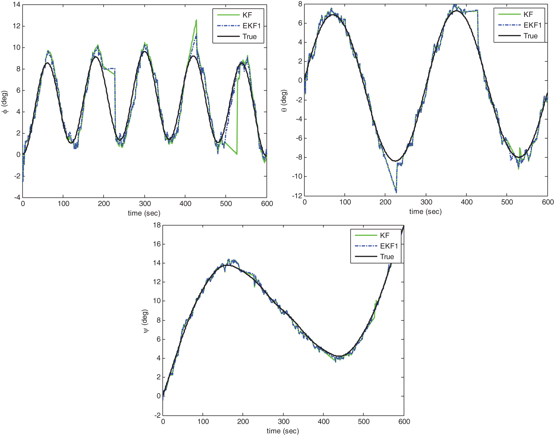
Figure 5: Estimate of attitude angles with signal outage: KF vs. EKF1

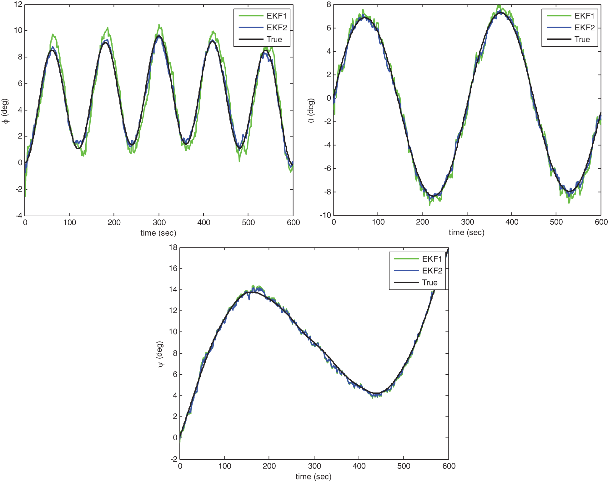
Figure 6: Estimate of attitude angles without signal outage: EKF1 vs. EKF2

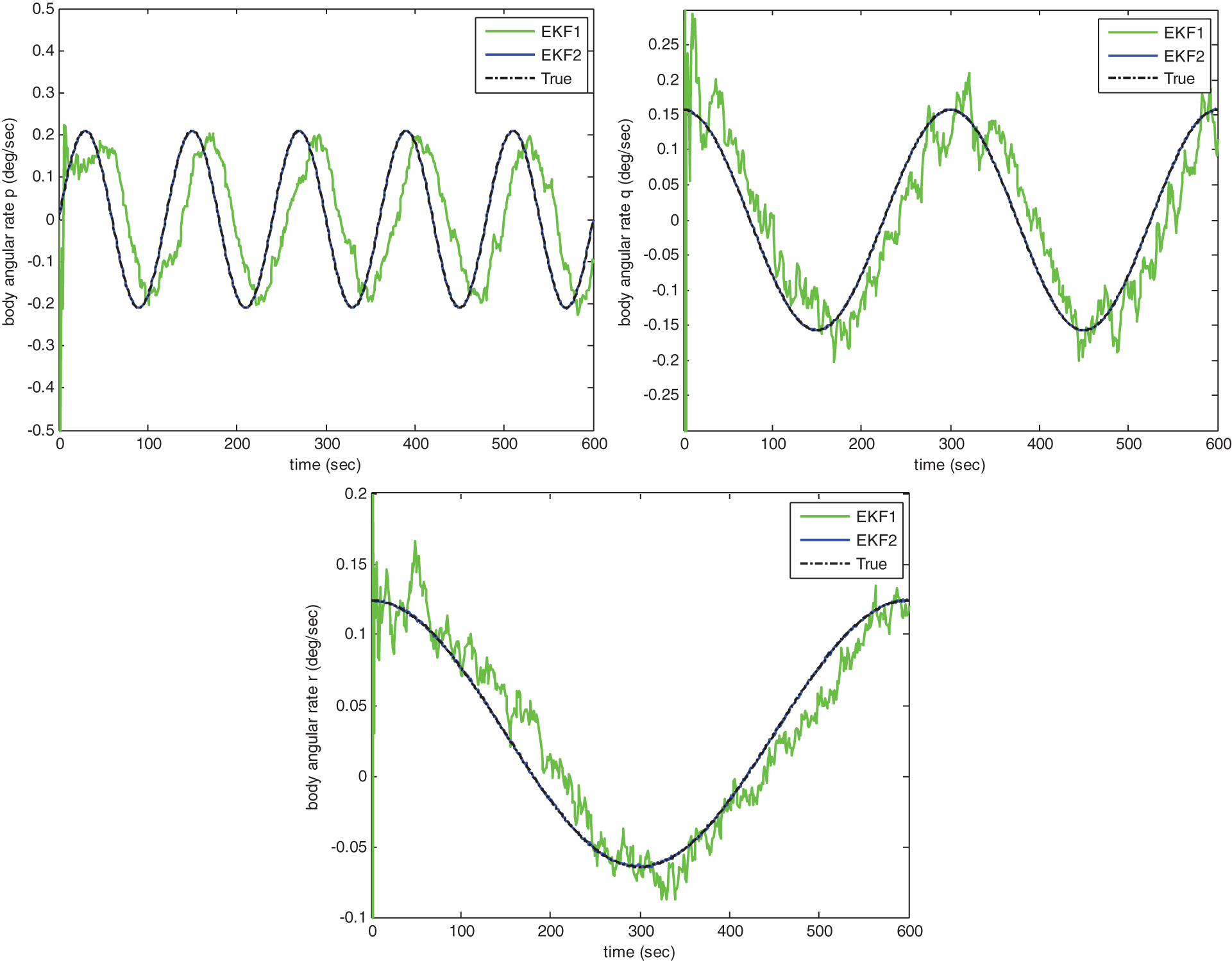
Figure 7: Estimate of body angular rates without signal outage: EKF1 vs. EKF2

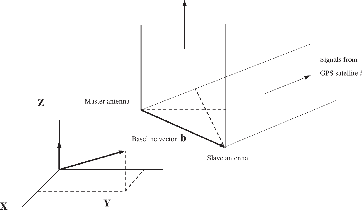
Figure 8: Estimate of attitude angles with signal outage: KF vs. EKF2

The above examples has demonstrated the attitude solutions obtained by KF and EKF based on measurements involving attitude angles only vs. those by EKF based on measurements involving both attitude angles and body angular velocities, possibly available from gyroscopes. In the case of signal outage, the body angular velocity is especially helpful from the view point of continuity of service and accuracy improvement.

5  Conclusions

The raw attitude solutions provided by the interferometry technique based on the least-squares approach are inherently noisy. The performance can be improved noticeably by using the Kalman family of filters. Incorporating the filter into the GPS interferometer effectively improves the performance in estimation performance. However, the case for GPS signal outage leads to performance degradation and even divergence. The proposed design provides the opportunity when body angular rates information from other sensor such as the gyroscopes is available for better resistance to the signal-challenged environment.

Details on dynamic models, including the CAV model as the second-order filter, and CAA model as the third-order filter, respectively, have been discussed. Numerical simulation has been carried out using the Kalman filter and extended Kalman filter, using the CAV model. Results involved include the estimate of attitude angles, attitude rates, and body angular velocities, for the cases with and without signal outages. Examples shown includes the attitude solutions obtained by KF and EKF based on measurements involving attitude angles only vs. those by EKF based on measurements involving both attitude angles and body angular velocities, possibly from gyroscopes. In the case of signal outage, the body angular velocity, possibly from gyroscopes is noticeably helpful from the view point of continuity of service and accuracy improvement.

Funding Statement: This work has been partially supported by the Ministry of Science and Technology, Taiwan [Grant Numbers MOST 109-2221-E-019-010 and MOST 110-2221-E-019-042].

Conflicts of Interest: The authors declare that they have no conflicts of interest to report regarding the present study.

References

 1.  K. Borre, D. M. Akos, N. Bertelsen, P. Rinder and S. H. Jensen, A Software-Defined GPS and Galileo Receiver, Boston, MA, USA: Birkhäuser, pp. 109–135, 2007. [Google Scholar]

 2.  B. Y. J. Tsui, Fundamentals of Global Positioning System Receivers: A Software Approach, Second Edition, New York, NY, USA: John Wiley & Sons, pp. 7–29, 2005. [Google Scholar]

 3.  D. Kaplan and C. J. Hegarty, Understanding GPS: Principles and Applications, Boston, MA, USA: Artech House, Inc., pp. 301–378, 2006. [Google Scholar]

 4.  P. Axelrad and R. G. Brown, Chapter 9 GPS Navigation Algorithms. In: B. W. Parkinson, J. J. Spilker, P. Axelrad and P. Enge (Eds.Global Positioning System: Theory and Applications, Washington, DC, USA: American Institute of Aeronautics and Astronautics, Inc., vol. 1, pp. 409–433, 1996. [Google Scholar]

 5.  B. Hofmann-Wellenhof, H. Lichtenegger and E. Wasle, GNSS–Global Navigation Satellite Systems, GPS, GLONASS, Galileo, and More, New York, NY, USA: Springer, pp. 309–340, 2008. [Google Scholar]

 6.  A. Raskaliyev, S. Hosi Patel, T. M. Sobh and A. Ibrayev, “GNSS-Based attitude determination techniques-a comprehensive literature survey,” IEEE Access, vol. 8, pp. 24873–24886, 2020. [Google Scholar]

 7.  L. M. Ryzhkov, “Using GPS for attitude determination,” in Proc. 2019 IEEE 5th Int. Conf. Actual Problems of Unmanned Aerial Vehicles Developments (APUAVD), Kyiv, Ukraine, pp. 199–201, 2019. [Google Scholar]

 8.  C. Erickson, “An analysis of ambiguity resolution techniques for rapid static GPS surveys using single frequency data,” in Proc. of the 5th Int. Technical Meeting of the Satellite Division of the Institute of Navigation (ION GPS 1992), Albuquerque, NM, USA, pp. 453–462, 1992. [Google Scholar]

 9.  H. Li, G. Nie, D. Chen, S. Wu and K. Wang, “Constrained MLAMBDA method for multi-GNSS structural health monitoring,” Sensors, vol. 19, no. 20, pp. 4462, 2019. [Google Scholar]

10. I. Al-Darraji, M. Derbali, H. Jerbi, F. Q. Khan, S. Jan et al., “A technical framework for selection of autonomous UAV navigation technologies and sensors,” Computers, Materials & Continua, vol. 68, no. 2, pp. 2771–2790, 2021. [Google Scholar]

11. Y. Li, M. Efatmaneshnik and A. G. Dempster, “Attitude determination by integration of MEMS inertial sensors and GPS for autonomous agriculture applications,” GPS Solutions, vol. 16, pp. 41–52, 2012. [Google Scholar]

12. J. A. Farrell and M. Barth, The Global Positioning System & Inertial Navigation, New York, NY, USA: McCraw-Hill, pp. 95–139, 1999. [Google Scholar]

13. P. Zhang, Y. Zhao, H. Lin, J. Zou and X. Wang et al., “A novel GNSS attitude determination method based on primary baseline switching for a multi-antenna platform,” Remote Sensing, vol. 12, no. 5, pp. 747, 2020. [Google Scholar]

14. M. Wei, M. E. Cannon and K. P. Schwarz, “Maintaining high accuracy GPS positioning on-the-fly,” in Proc. of IEEE Position Location and Navigation Symp. (PLANS), Monterey, CA, USA, pp. 403–411, 1992. [Google Scholar]

15. F. Van Grass and M. Braasch, “GPS interferometric attitude and heading determination: Initial flight test results,” Navigation, vol. 38, no. 4, pp. 359–378, 1991–1992. [Google Scholar]

16. B. J. Muth, P. J. Oonincx and C. C. J. M. Tiberius, “Differential observables for software-based GPS interferometry,” in Proc. 17th European Signal Processing Conf. (EUSIPCO), Glasgow, Scotland, pp. 2166–2170, 2009. [Google Scholar]

17. L. Lu, L. Ma, T. Wu and X. Chen, “Performance analysis of positioning solution using low-cost single-frequency u-blox receiver based on baseline length constraint,” Sensors, vol. 19, no. 19, pp. 4352, 2019. [Google Scholar]

18. A. Hauschild, O. Montenbruck and R. B. Langley, “Flight results of GPS-based attitude determination for the Canadian CASSIOPE satellite,” Navigation, vol. 67, no. 1, pp. 83–93, 2020. [Google Scholar]

19. R. G. Brown and P. Y. C. Hwang, Introduction to Random Signals and Applied Kalman Filtering, New York, NY, USA: John Wiley & Sons, pp. 190–241, 1997. [Google Scholar]

20. H. G. de Marina, F. J. Pereda, J. M. Giron-Sierra and F. Espinosa, “UAV attitude estimation using unscented Kalman filter and TRIAD,” IEEE Transactions on Industrial Electronics, vol. 59, no. 11, pp. 4465–4474, 2012. [Google Scholar]

21. L. Wang, Z. Zhang and P. Sun, “Quaternion-based Kalman filter for AHRS using an adaptive-step gradient descent algorithm,” International Journal of Advanced Robotic Systems, vol. 12, no. 9, pp. 131–143, 2015. [Google Scholar]

22. R. B. Widodo and C. Wada, “Attitude estimation using Kalman filtering: External acceleration compensation considerations,” Journal of Sensors, vol. 2016, article ID 6943040, pp. 24, 2016. [Google Scholar]

23. A. Deibe, J. A. A. Nacimiento, J. Cardenal and F. L. Pena, “A Kalman filter for nonlinear attitude estimation using time variable matrices and quaternions,” Sensors, vol. 20, no. 23, pp. 6731, 2020. [Google Scholar]

24. GPSoft LLC., Satellite Navigation Toolbox 3.0 User's Guide, Athens, OH, USA, 2003. [Google Scholar]

This work is licensed under a Creative Commons Attribution 4.0 International License, which permits unrestricted use, distribution, and reproduction in any medium, provided the original work is properly cited.