Computers, Materials & Continua DOI:10.32604/cmc.2022.019681
Article

Modeling and Simulation of Two Axes Gimbal Using Fuzzy Control

Ayman A. Aly1, Mohamed O. Elhabib2, Bassem F. Felemban1, B. Saleh1 and Dac-Nhuong Le3,4,*

1Department of Mechanical Engineering, College of Engineering, Taif University, Taif, 21944, Saudi Arabia
2Control and Mechatronics Division, School of Electrical Engineering, UTM, Johor Bahru, 81300, Malaysia
3Institute of Research and Development, Duy Tan University, Danang, 550000, Vietnam
4School of Computer Science, Duy Tan University, Danang, 550000, Vietnam
*Corresponding Author: Dac-Nhuong Le. Email: ledacnhuong@duytan.edu.vn
Received: 21 April 2021; Accepted: 23 November 2021

Abstract: The application of the guided missile seeker is to provide stability to the sensor's line of sight toward a target by isolating it from the missile motion and vibration. The main objective of this paper is not only to present the physical modeling of two axes gimbal system but also to improve its performance through using fuzzy logic controlling approach. The paper is started by deriving the mathematical model for gimbals motion using Newton's second law, followed by designing the mechanical parts of model using SOLIDWORKS and converted to xml file to connect dc motors and sensors using MATLAB/SimMechanics. Then, a Mamdani-type fuzzy and a Proportional-Integral-Derivative (PID) controllers were designed using MATLAB software. The performance of both controllers was evaluated and tested for different types of input shapes. The simulation results showed that self-tuning fuzzy controller provides better performance, since no overshoot, small steady-state error and small settling time compared to PID controller.

Keywords: Gimbal system; self-tuning fuzzy; proportional-integral-derivative (PID) control; cross coupling

1  Introduction

Weapon history has evolved in tandem with human history. Recent weapon systems are evolving to cause the least amount of human harm and to neutralize military facilities. The primary goal of a missile is too accurately to shoot the moving and fixed targets. As a result, it has been steadily producing missiles that use different seeker technologies. The seeker system's function is to actively track up to the target by detecting and locking on to the object. In this system, there are many sources of noise and disturbances, which come from vibrations of the seeker and maneuvering of the missile while flighting, also there is a decoupling in the line of sight (LOS) between the seeker and the object. So, it is realized that the seeker consists of a two-axis gimbal platform to track stably and make a stabilization loop [1].

In the two-axis gimbal system, dc motors are connected to each axis as actuating parts, for the sensing part, two sensors are used a gyro is used to measure the speed and position sensor for angle measuring. To avoid disturbance and measure stable values, sensors are located on the inner gimbal. Most disturbances result from missile motions, gimbal system geometry, and gimbal system imperfections like mass unbalance [2]. Therefore, the dynamics of the plant must be expressed in analytical form before the design of the gimbal system is taken up. The mathematical model and control system of two axes gimbal system has been studied by many research. Rue [3] presented the kinematics and geometrical coupling relationships for two degrees of freedom gimbal assembly for a simplified case when each gimbal is balanced. In [4], Ekstrand derived the equations of motion for the two axes gimbal configuration by assuming the gimbals have no mass imbalance and inertia disturbances and cross-couplings can be eliminated by certain inertia symmetry conditions. For one degree of freedom gimbal studied in [5], the static and dynamic imbalance disturbance torques created by the vibrations of the operating environment can be eliminated by statically and dynamically balancing the gimbal, which is regarded costly and time-consuming.

On the other hand, many controllers were designed and studied for years to stabilize the gimbal system. Nonlinear controllers such as, in [6] Sliding Mode Controller (SMC) is used under the assumption of uncoupled identical elevation and azimuth, although the controller was able to provide good results in terms of control design specifications, it lacks the simplicity of the design. In [7] authors presented a novel control approach to improve the performance of the system against internal and external disturbances, which consists of a backstepping controller, nonlinear disturbance observer, and two third-order reference models. According to simulation results, the controller improved the angular velocity precision and accurately tracks the desired rotation angles and angular velocities with very good transient and steady-state responses. Altan [8] used Model Predictive Control (MPC) with Hammerstein model to improve real time target tracking performance under external disturbance for a three-axis gimbal system. Based on the simulation and experimental results he found MPC algorithm with Hammerstein model provided good tracking to the target while maintaining the stability under external disturbances compared to the PID controller. Linear and optimal controllers (PID, Linear Quadratic. Regulator (LQR)) are limited to linear systems, and much tuning for parameters is required to obtain good performance and is difficult to be realized. Recently fuzzy logic controlling approach has been developed to improve the performance of the system and to deal with nonlinear models and uncertainties [9,10]. Therefore, this paper will focus on the designing of an intelligent controller (fuzzy logic controller) for a two-axis gimbal system and the PID controller will be used for comparison purposes.

This paper is organized as follows, it started by derivation the mathematical model of the system by using Lagrange equations followed by 3D physical modeling of two-axis gimbal using MATLAB Simscape, after that fuzzy logic controller based Mamdani type designed for inner and outer loops. Finally, the simulation results of both fuzzy and PID controllers are presented.

2  Mathematical Modeling

Let the figure of under consideration system as shown as in Fig. 1.

Figure 1: Two axis gimbal system

It contains a body with outer and inner gimbals such that the tracking sensor is mounted on the inner gimbal. In this regard, three references frames can be defined as body frame B, outer frame O, and inner frame I. The coordinate axes of these frames are {XB,YB,ZB}, {XO,YO,ZO}, and {XI,YI,ZI} respectively. As it is seen in figure φ is the rotation angle of outer frame about the ZO axis in the positive direction with respect to the body frame, and θ is the rotation angle of the inner frame about the outer frame about YI axis.

Let LOB is the transformation from B to O and LIO is the transformation from O to I, the transformation matrices will be:

LOB=[cos⁡∅sin⁡∅0−sin⁡∅cos⁡∅0001](1)

LIO=[cos⁡θ0−sin⁡θ010sin⁡θ0cos⁡θ](2)

For the inertial angular velocities of frame B, O, and I with respect to themselves, the following vectors are introduced:

ω¯B=[pqr],ω¯O=[poqoro],ω¯I=[piqiri](3)

p, q, and r are stands for roll, pitch, and yaw respectively, as usual notations in the flight system.

JI=[JixDxyDxzDxyJiyDyzDxzDyzJiz],JO=[JoxdxydxzdxyJoydyzdxzdyzJoz](4)

J represents the moment of inertia and product of inertia denoted by D or d. If we assumed that the center of the gimbal is in the common center of rotation, then there is no mass unbalance in the gimbals. If we consider the stabilization loop of the system, with the above notations, the aim is to keep the sensor non-rotating in the inertial space in the presence of the disturbances, which is achieved by keeping qi=ri=0.qi and ri can be measured in two ways; the first way by fixing a two-axis rate gyro on the inner gimbal. The other way is to use body-fixed rate gyros and using the gimbal angles ∅ and θ. For this, consider the following vector:

φ˙¯=[00∅˙],ϑ˙¯=[0θ˙0](5)

From the above equation, the relations between angular velocities of the outer gimbal, body, and inner gimbal are as follow:

ω¯O=LOB+φ˙¯(6)

ω¯I=LIO+ϑ˙¯(7)

From Eqs. (6) and (7), the angular velocities of the outer and inner gimbals will be as follows:

ω¯O=[pcos⁡∅+qsin⁡∅−psin⁡∅+qcos⁡∅r+∅˙](8)

ω¯I=[pcos⁡θ−rosin⁡θqo+θ˙posin⁡θ+rocos⁡θ](9)

2.1 Equation of Motion about the Pitch Axis

The gimbal dynamics model can be derived from the torque relationships about the inner and outer gimbals. The equation of motion for the inner gimbal can be expressed as follows:

T¯I(t)=[TIx(t)TIy(t)TIz(t)]=JIω˙¯I(t)+(ω¯I(t)∗JIω¯I(t))+[TUIx(t)TUIy(t)TUIz(t)]+[0TIfω(t)0](10)

where TUIx(t), TUIy(t), and TUIz(t) are the mass unbalance torque about the inner gimbal axes, TIy(t) is the applied control torque, TIx(t), TIz(t) are the reaction torque between inner and outer gimbal, and TIfω(t) stands for the friction and cable restraint torque and can be generate both linear and nonlinear disturbance as follows:

TIfw=TI,fric+TI,CR+KIfθ˙+KIwθ(11)

The inner gimbal motion equation about the pitch axis can be expressed as:

TIy=Jiyq˙i+KIfθ˙+KIwθ+TI,fric+TI,CR+TUIy+TD(12)

where TIy is the external torque about the pitch axis TI,fric and TI,CR are non-linear friction and non-linear cable restraint torque respectively, KIf, KIw are the viscous friction and cable restraint coefficients respectively, and TD is the undesired external disturbance torques due to the inertial terms as:

TD=(Jiz− Jix )piri+ Dxz(pi2− ri2)− Dyz(r˙i+ piqi)−Dxy(p˙i+qiri) (13)

The relation (14) can be considered with some approximation, and it is seen that how the disturbance torques due to the inertial terms can be vanished. For instance, if the products of the inertia are negligible and moments of inertia Jix and Jiz be equal, that is,

Dxy=Dxz= Dyz=0(14)

Jix= Jiz(15)

Then, TD is equal zero. In the procedure of the design, it should be tried satisfying the condition (14) and (15) in order to delete the disturbance due to the inertial terms. By using the relation (9), the Eq. (14) can be rewritten as:

TD=TB+ TC(16)

where,

TB= −(Dyzsinθ+ Dxycos⁡θ)(p˙0+q0r0)+(Dyzcosθ−Dxysinθ)p0q0+[(Jiz−Jix)cos (2θ)−2Dxzsin(2θ)]p0r0+ 12[(Jiz− Jix)sin⁡(2θ)+2Dxzcos(2θ)]p02(17)

TC=−(Dxysinθ− Dyzcos⁡θ)r˙0−12[(Jiz−Jix)sin⁡(2θ)+2Dxzcos(2θ)]r02(18)

If the body is non-rotating, i.e., p= q=r=0, then from the relation (8) we have p0= q0=0 and TB will be zero. However, TC is not necessarily zero and the motion of the outer gimbals. In the control point of view, TC related to the cross couplings between two axes, and TB is the disturbance due to the rotation of the body. It is obvious that if Eqs. (14) and (15) are satisfied, both terms will vanish.

2.2 The Equation of Motion about the Yaw Axis

The equation of motion for outer gimbal can be expressed as:

T¯O(t)=[TOx(t)TOy(t)TOz(t)]=(JOω˙¯O(t)+(ω¯O(t)× JOω¯O(t))+[Ti(t)]O)−[TUOx(t)TUOy(t)TUOz(t)]−[00TOfω(t)](19)

In which, all the parameters and coefficients are defined as a similar manner in the Section (2.1) and TOfw(t) again can be written as:

TOfw(t)= TO.fric+TO.CR+KOw(∅)(20)

TOz(t)=JSr˙O+KOf∅˙+KOwφ+TO,CR+TUOz+TD(21)

where TOz is the external torque about the yaw axis and other coefficients are as before with suitable index, JS is the total moment of inertia about the outer gimbal Zo axis. If the inner gimbal rotates, angle θ will change and therefore JS is an instantaneous moment of inertia about Zo axis dependent upon θ variations as follows:

Js = Joz+Jix sin2 θ + Jizcos2θ−Dxzsin(2θ) (22)

The external undesired disturbance torques TD in Eq. (21) can be considered as:

Td = Td1−Td2−Td3(23)

where,

Td1= [Jox+ Jix cos2θ + Jiz sin2θ+ Dxzsin(2θ)− (Joy+Jiy)]po qo(24)

Td2=−[dxz+(Jiz+Jix)sinθcosθ+Dxzcos(2θ)](po⋅−qoro)−(dyz+Dyzcosθ−Dxysinθ(qo⋅+poro))−dxy+Dxycosθ−Dyzsinθ(po2−qo2)(25)

Td3=θ¨(Dxysinθ−Dyzcosθ)+θ˙[(Jix−Jiz)(pocos⁡(2θ)−rosin⁡(2θ))+2Dxz(posin⁡(2θ))+rocos⁡(2θ)+(Dyzsinθ+Dxycos⁡θ)(qi+qo)−Jiypo](26)

These terms of disturbance torque can be interpreted as follows. Suppose the rotation angle of θ is constant, i.e., θ˙=0. It is resulted that Td3+0. Relations (24) and (25) indicate that Td1 and Td2 are the disturbance terms of equation motion of the rigid body for the gimbal system about Zo  axis. Td1 is due to the difference of the moments of inertia and Td2 comes from the products of inertia and both are dependent upon θ. However, in the case of that θ is varying, the gimbal system is not further a rigid body and an extra term is produced, Td3, which affects the equation of motion. In this case also, we can consider the conditions which cause disturbance rejection. Most of the disturbance terms in relations (24)–(26) can be deleted by satisfying the following conditions:

Dxy=Dxz=Dyz=0(27)

Jix=Jiz(28)

Js=Joz− Jiz(29)

Td1= [(Jox+ Jix)− (Joy+Jiy)]po qo(30)

Td2=0(31)

Td3= −Jiy θ˙.po(32)

By using the relation θ˙=qi−qo, the sum of the disturbances terms is:

Td1+Td2+Td3=(Jox+Jix−Joy)poqo−Jiypoqi (33)

If the mechanical design is such that the condition (34) is satisfied, then the total disturbance reduce to Jiy poq, which cannot be deleted.

Joy = Jix+ Jox (34)

The last manipulation which should be done on the derived equation of the outer gimbal is to rewrite the equation according to the ri instead of ro since ri is the controlled output variable. This can be simply accomplished by using the relations (8) and (9). In the similar manner of the inner gimbal, the TD can be interpreted by introducing the cross coupling.

By using relation θ˙=qi−qo, TD is rewritten as:

Td=Tb+Tc(35)

where,

Td=Td1+Td2+θ˙[(Jix−Jiz)cos⁡(2θ)+2Dxzsin⁡(2θ)−Jiy]po+[(Jix−Jiz)sin⁡(2θ)+2Dxzcos⁡(2θ)]qoro+(Dyzcos⁡θ−Dxysinθ)q˙o−(Dyxsinθ+Dxycosθ)qo2(36)

Tc=(Dxysinθ−Dyzcosθ)q˙i+(Dxycosθ+Dyzsinθ)qi2+[(Jiz−Jix)sin⁡(2θ)+2Dxzcos(2θ)]qiro(37)

For a non-rotating body p, q, and r are zero and we have po=qo=0, which results in Tb = 0. However, even in this case there is a cross coupling term Tc which is due to the inner gimbal motion. Tc will be zero if conditions (27) and (28) are satisfied.

3  Physical Modeling

Physical modeling is a way of modeling and simulating systems that consist of real physical components. It employs a physical network approach, where Simscape blocks correspond to physical elements, such as pumps, motors, and op-amps. By joining these blocks by lines corresponding to the physical connections that transmit power. This approach can describe the physical structure of a system, instead of linear and nonlinear equations. These virtual devices can drastically reduce the cost of testing control systems, software, and hardware. It can also improve the quality of the final product by enabling more complete testing of the entire system. SOLIDWORKS was used to design the gimbal, which consists of 3 parts as in Figs. 2 and 3 and connected by two revolute joints. Each joint was driven by a dc-motor (not shown in the figures below) via a gearbox. The mounting point of the camera on the body (3) in the θ direction.

Figure 2: Two axis gimbal Simscape diagram

Figure 3: Two axis gimbal SOLIDWORKS design

4  Fuzzy Controller Design

Fuzzy logic and fuzzy sets have been around now for more than 20 years. In 1965, Zadeh first proposed fuzzy sets, which are considered as an approach to processing data, and they became popular in the different fields of science. In (1974) Mamdani presented a fuzzy controller method and it gained high popularity in the engineering field [11–20]. Fuzzy Logic similar to the human decision-making methodology deals with vague and imprecise information.

Thus, it is easier to understand since its working principle depends on the linguistic statements. The fuzzy controller comprises four main phases, which are the fuzzification phase where the input values are converted to a fuzzy variable (linguistic variables). In this paper we used two input variables to control the dc motors, which are error (e) of the dc motor motion, and its derivative error (e.) with three fuzzy subsets are both, which are [H M L] and [N Z P] respectively, by using three Gaussian membership functions as in Figs. 4a and 4b.

The output has five subsets represented using z-membership functions as shown in Fig. 5, the subsets are [FC SC NC OS OF], where FC is fast close, SC is slow to close, NC is no change, OS is open slow, and FC is open fast. For the Fuzzy inference system, the MAX-MIN approach was used to determine the degree of membership function of the output variables. In the defuzzification phase, all the consequents were aggregated to obtain a crisp output in order to produce a non-fuzzy control that best represents the degree of certainty of an inferred fuzzy control action. They are several numbers of procedures of defuzzification the rules output-aggregate for the Mamdani method. In this project Center of gravity was used because it is considered the most efficient in that it gives a defuzzification output.

Figure 4: (a) Membership function of the error; (b) Membership function of the derivative error

Figure 5: Output membership function

5  Simulation Results

The two axes gimbal system is validated using MATLAB/Simulink environment is depicted with SimMechanics model in Fig. 2. A comparison of the proposed self-tuning fuzzy controller and conventional PID is carried out using step input commands in elevation and azimuth axes. As an example, one case of system response is displayed in Figs. 6a and 7a, respectively. The response of elevation illustrates that the rise time of PID control is 0.086 s with a small overshoot amplitude of 0.5% and for fuzzy it was 0.011 s with no overshoots while the steady-state error also improved from 0.0015 to be 0.001. The azimuth response with different step input amplitude assured the superiority of the proposed self-tuning fuzzy compared with the traditional PID. The rise time decreased from 0.093 s to be 0.013 s and the overshoot amplitude is changed from 0.063% to be nearly zero also the steady-state error decrease from 0.006 to be 0.002. The angle rates obtained from the derivation of the angle positions are shown in Figs. 6c and 7c. It is clear that the PID controller creates an overshoot and increases settling time. While a fuzzy controller can meet the variation of angle position and improve the transient and steady-state performance by achieving fast response with no overshoot as compared to conventional PID.

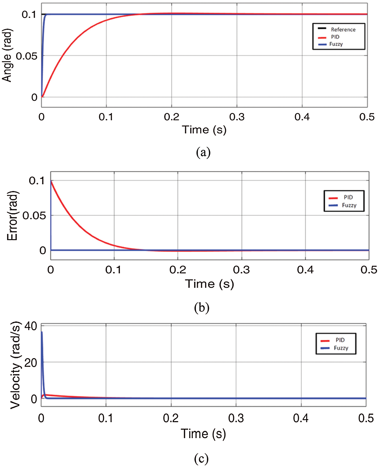
Figure 6: (a) The gimbal elevation step response for angular input; (b) the error signal; (c) the angular rate signal

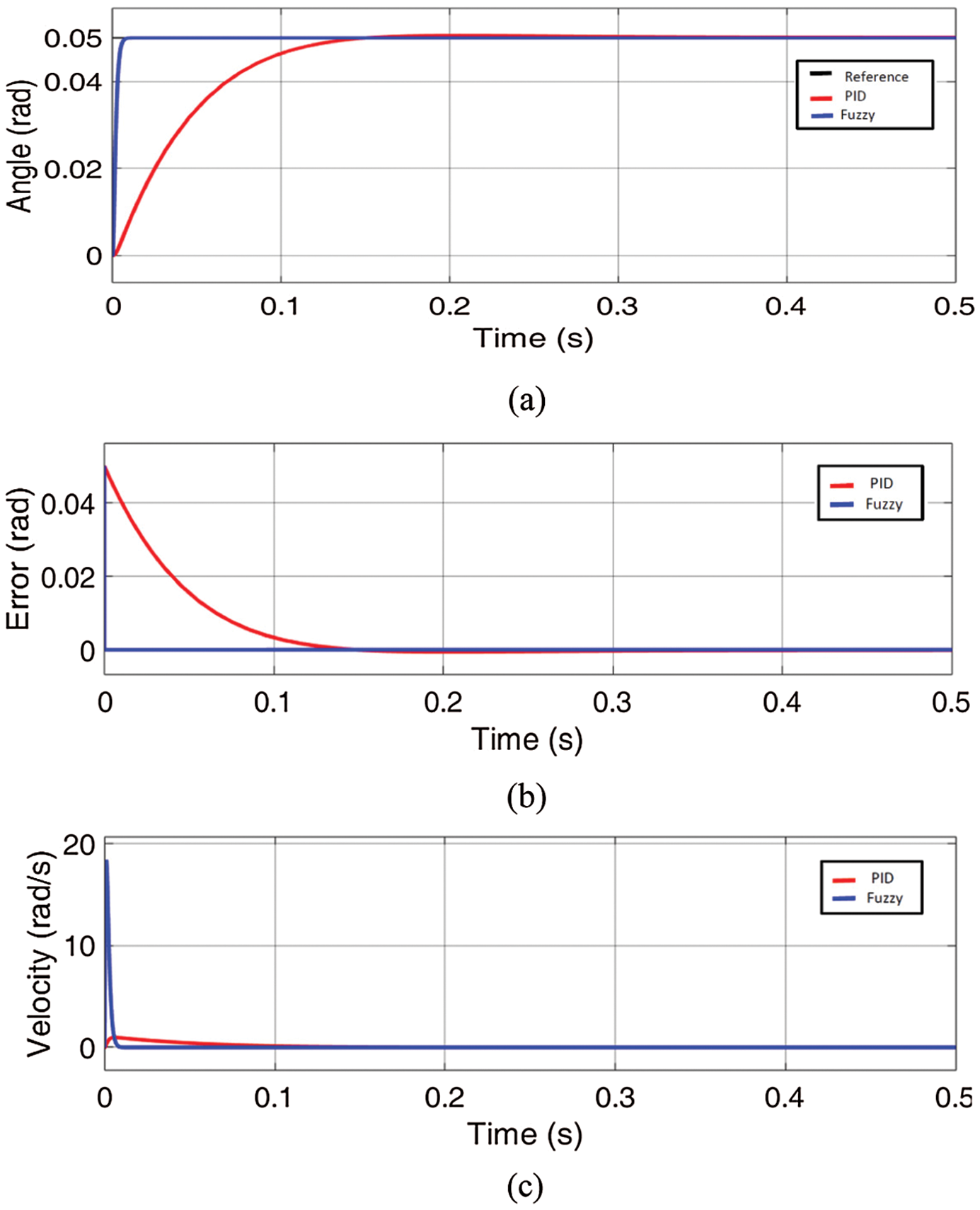
Figure 7: (a) The gimbal azimuth step response for angular input; (b) the error signal; (c) the angular rate signal

To confirm this efficiency, many comparison tests indicated using different inputs shapes.

In the following figures, a sin waves input is applied with different amplitudes for elevation and azimuth axes. The elevation axis response gave an error of 5.24 × 10−3 with PID control and 0.15 × 10−3 with fuzzy control while the azimuth response gave an error of 0.014 with PID control and 0.003 with fuzzy control. The error and control signal presented in Figs. 8c and 9c.

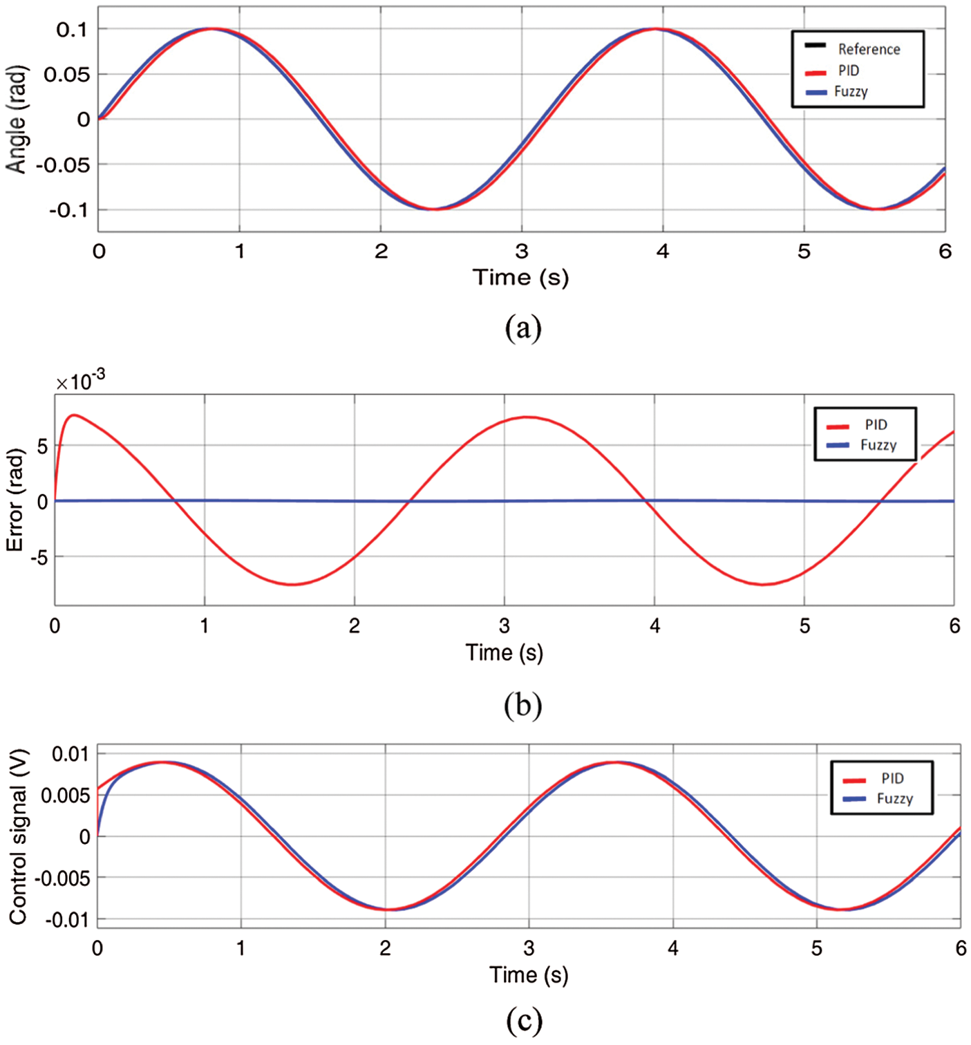
Figure 8: (a) The gimbal elevation sinusoidal response for angular input; (b) the error signal; (c) the controllers signals

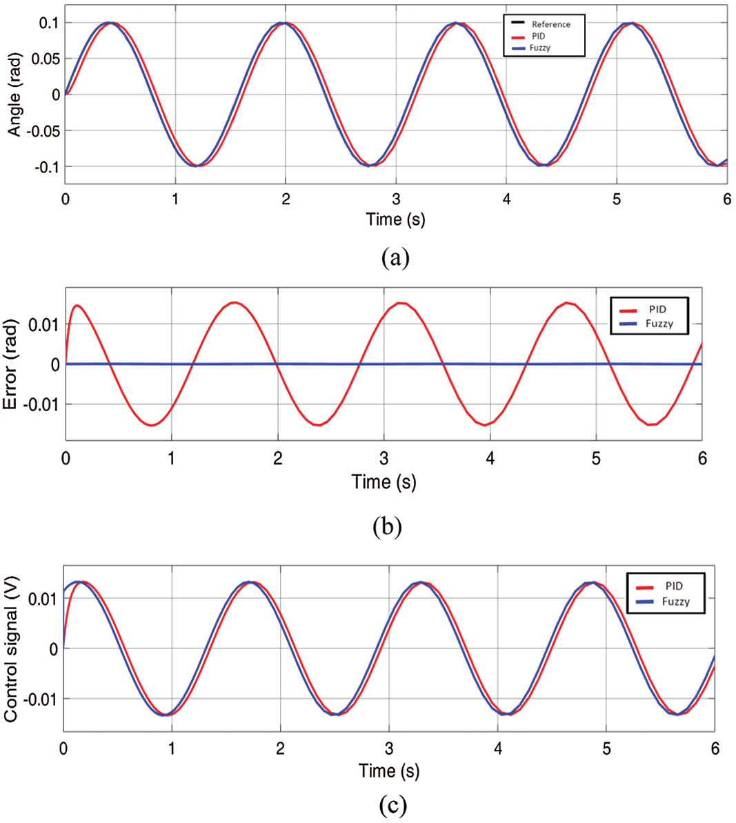
Figure 9: (a) The gimbal azimuth sinusoidal response for angular input; (b) the error signal; (c) the controllers signals

With the help of the control parameters of the electromechanical simulation model, the proposed fuzzy controller can track the command angle rapidly and accurately, by which high stabilization performance can be attained.

Due to fact, the elevation axis of the system is compatible with the azimuth axis to produce the final motion of the system. Therefore, it is necessary to test the control performance under movable base conditions by simulating the axes at various angles. In Fig. 10 the input to elevation is sin wave and for elevation is cosine wave which finally produces a complete circle.

Previous results clearly reflect the efficiency of the self-tuning fuzzy controller compared to the conventional PID. The test assures the superiority of the proposed fuzzy compared with the classical PID control. It has good tracking accuracy whether for azimuth gimbal or elevation gimbal.

Figure 10: The gimbal response for elevation sin and azimuth cosine inputs

6  Conclusion

In this paper, a two axes gimbal system was proposed and formulated utilizing Newton's second law. The equations for the gimbals’ motion were derived and introduced in two formulations according to the dynamic mass unbalance. The gimbal system was simulated using MATLAB/SimMechanics. A comparison between the system responses with different inputs shapes was made and the comparison results verified the proposed model. The responses have been analyzed, then the performance of the Self-tuning fuzzy controller has been tested using transient response analysis and a quantitative study of error analysis. Based on the obtained results, some observations can be cleared.

The proposed self-tuning fuzzy control provides good adaptivity to the gimbal system which offers high performance so that it can be utilized more efficiently in the dynamical environment that usually imposes large variable base rates. It is clear that the proposed fuzzy controller can reduce the response settling time as compared with the conventional PID controller.

Finally, the proposed fuzzy controller improves the closeness of System response and supports the system relative stability by reducing the response overshoot considerably without increasing the response rise time dramatically.

Acknowledgement: Taif University Researchers Supporting Project number (TURSP-2020/260), Taif University, Taif, Saudi Arabia.

Funding Statement: The authors would like to thank the Deanship of Scientific Research at Taif University for the grant received for this research. This research was supported by Taif University with research grant TURSP-2020/260, https://www.tu.edu.sa/En/Deanship-of-Scientific-Research/83/News/22911/Researchers-Supporting-Project-(TURSP).

Conflicts of Interest: The authors declare that they have no conflicts of interest to report regarding the present study.

References

 1.  K. J. Seong, H. G. Kang, B. Y. Yeo and H. P. Lee, “The stabilization loop design for a two-axis gimbal system using LQG/LTR controller,” in 2006 SICE-ICASE Int. Joint Conf., Busan, Korea, pp. 755–759, 2006. [Google Scholar]

 2.  M. Abdo, A. R. Vali, A. R. Toloei and M. R. Arvan, “Modeling control and simulation of two axes gimbal seeker using fuzzy PID controller,” in 2014 22nd Iranian Conf. on Electrical Engineering (ICEE), Tehran, Iran, pp. 1342–1347, 2014. [Google Scholar]

 3.  A. K. Rue, “Precision stabilization systems,” IEEE Transactions on Aerospace and Electronic Systems, vol. 1, pp. 34–42, 1974. [Google Scholar]

 4.  B. Ekstrand, “Equations of motion for a two-axes gimbal system,” IEEE Transactions on Aerospace and Electronic Systems, vol. 37, no. 3, pp. 1083–1091, 2001. [Google Scholar]

 5.  D. R. Otlowski, K. Wiener and B. A. Rathbun, “Mass properties factors in achieving stable imagery from a gimbal mounted camera,” in Airborne Intelligence, Surveillance, Reconnaissance (ISR) Systems and Applications V, vol. 6946, pp. 69460B, 2008. [Google Scholar]

 6.  B. J. Smith, W. J. Schrenk, W. B. Gass and Y. B. Shtessel, “Sliding mode control in a two-axis gimbal system,” in Proc. of 1999 IEEE Aerospace Conf., Cat. No. 99TH8403, Snowmass, CO, USA, vol. 5, pp. 457–470, 1999. [Google Scholar]

 7.  L. Mihai, “Control of double gimbal control moment gyro systems using the backstepping control method and a nonlinear disturbance observer,” Acta Astronautica, vol. 180, pp. 639–649, 2021. [Google Scholar]

 8.  A. Altan and R. Hacıoğlu, “Model predictive control of three-axis gimbal system mounted on UAV for real-time target tracking under external disturbances,” Mechanical Systems and Signal Processing, vol. 138, pp. 106548, 2020. [Google Scholar]

 9.  C. Y. Li and W. X. Jing, “Fuzzy PID controller for 2D differential geometric guidance and control problem,” IET Control Theory & Applications, vol. 1, no. 3, pp. 564–571, 2007. [Google Scholar]

10. D. Dubois and H. Prade (Eds.Fundamentals of Fuzzy Sets. Springer Science & Business Media, Switzerland AG, 2012. [Google Scholar]

11. T. K. Madhubala, M. Boopathy, J. S. Chandra and T. K. Radhakrishnan, “Development and tuning of fuzzy controller for a conical level system,” in Proc. of Int. Conf. on Intelligent Sensing and Information Processing, Chennai, India, pp. 450–455, 2004. [Google Scholar]

12. A. A. Hamad, A. S. Al-Obeidi, E. H. Al-Taiy, O. I. Khalaf and D. Le, “Synchronization phenomena investigation of a new nonlinear dynamical system 4d by gardano's and lyapunov's methods,” Computers, Materials & Continua, vol. 66, no. 3, pp. 3311–3327, 2021. [Google Scholar]

13. M. M. Abdo, A. R. Vali, A. R. Toloei and M. R. Arvan, “Stabilization loop of a two axes gimbal system using self-tuning PID type fuzzy controller,” ISA Transactions, vol. 53, no. 2, pp. 591–602, 2014. [Google Scholar]

14. H. Khodadadi and H. Ghadiri, “Self-tuning PID controller design using fuzzy logic for half car active suspension system,” International Journal of Dynamics and Control, vol. 6, no. 1, pp. 224–232, 2018. [Google Scholar]

15. A. Naderolasli and M. Tabatabaei, “Two-axis gimbal system stabilization using adaptive feedback linearization,” Recent Advances in Electrical & Electronic Engineering, vol. 12, pp. 1–11, 2019. [Google Scholar]

16. A. Naderolasli and M. Ataei, “Stabilization of a two-dof gimbal system using direct self-tuning regulator,” International Journal on Electrical Engineering and Informatics, vol. 12, no. 1, pp. 33–44, 2020. [Google Scholar]

17. D. N. Le, A. K. Pandey, S. Tadepalli, P. S. Rathore and J. M. Chatterjee, Network Modeling, Simulation and Analysis in MATLAB: Theory and Practices. John Wiley & Sons, USA, 2019. [Google Scholar]

18. A. A. Hamad, A. S. Al-Obeidi, E. H. Al-Taiy, O. I. Khalaf and D. Le, “Synchronization phenomena investigation of a new nonlinear dynamical system 4d by gardano's and lyapunov's methods,” Computers, Materials & Continua, vol. 66, no. 3, pp. 3311–3327, 2021. [Google Scholar]

19. D. N. Le, G. N. Nguyen, H. Garg, Q. T. Huynh, T. N. Bao et al., “Optimizing bidders selection of multi-round procurement problem in software project management using parallel max-min ant system algorithm,” Computers, Materials & Continua, vol. 66, no. 1, pp. 993–1010, 2021. [Google Scholar]

20. R. Singh and B. Bhushan, “Improving self-balancing and position tracking control for ball balancer application with discrete wavelet transform-based fuzzy logic controller,” International Journal of Fuzzy Systems, vol. 23, pp. 27–41, 2021. [Google Scholar]

This work is licensed under a Creative Commons Attribution 4.0 International License, which permits unrestricted use, distribution, and reproduction in any medium, provided the original work is properly cited.