Computers, Materials & Continua DOI:10.32604/cmc.2022.020244
Article

An Optimal Deep Learning for Cooperative Intelligent Transportation System

K. Lakshmi1, Srinivas Nagineni2, E. Laxmi Lydia3, A. Francis Saviour Devaraj4, Sachi Nandan Mohanty5, Irina V. Pustokhina6,* and Denis A. Pustokhin7

1Department of Computer Science and Engineering, Periyar Maniammai Institute of Science & Technology, Thanjavur, 613403, India
2Department of Computer Science and Engineering, KG Reddy College of Engineering and Technology, Telangana, 500075, India
3Department of Computer Science and Engineering, Vignan’s Institute of Information Technology (Autonomous), Visakhapatnam, 530049, India
4Department of Computer Science and Engineering, Kalasalingam Academy of Research and Education, Krishnankoil, 626128, India
5Department of Computer Engineering, College of Engineering Pune, Pune, Maharashtra, 411005, India
6Department of Entrepreneurship and Logistics, Plekhanov Russian University of Economics, Moscow, 117997, Russia
7Department of Logistics, State University of Management, Moscow, 109542, Russia
*Corresponding Author: Irina V. Pustokhina. Email: ivpustokhina@yandex.ru
Received: 15 May 2021; Accepted: 16 June 2021

Abstract: Cooperative Intelligent Transport System (C-ITS) plays a vital role in the future road traffic management system. A vital element of C-ITS comprises vehicles, road side units, and traffic command centers, which produce a massive quantity of data comprising both mobility and service-related data. For the extraction of meaningful and related details out of the generated data, data science acts as an essential part of the upcoming C-ITS applications. At the same time, prediction of short-term traffic flow is highly essential to manage the traffic accurately. Due to the rapid increase in the amount of traffic data, deep learning (DL) models are widely employed, which uses a non-parametric approach for dealing with traffic flow forecasting. This paper focuses on the design of intelligent deep learning based short-term traffic flow prediction (IDL-STFLP) model for C-ITS that assists the people in various ways, namely optimization of signal timing by traffic signal controllers, travelers being able to adapt and alter their routes, and so on. The presented IDL-STFLP model operates on two main stages namely vehicle counting and traffic flow prediction. The IDL-STFLP model employs the Fully Convolutional Redundant Counting (FCRC) based vehicle count process. In addition, deep belief network (DBN) model is applied for the prediction of short-term traffic flow. To further improve the performance of the DBN in traffic flow prediction, it will be optimized by Quantum-behaved bat algorithm (QBA) which optimizes the tunable parameters of DBN. Experimental results based on benchmark dataset show that the presented method can count vehicles and predict traffic flow in real-time with a maximum performance under dissimilar environmental situations.

Keywords: Cooperative intelligent transportation systems; traffic flow prediction; deep belief network; deep learning; vehicle counting

1  Introduction

Cooperative Intelligent Transport System (C-ITS) is a well-known and effective model which aspires to enhance road safety, traffic control, and driver security. It is the internal component used in future progressiveness of modern cities. A principle used in C-ITS has unique connectivity of vehicles and be aware of traffic rules. Using the vehicle to vehicle connectivity, Road Side Units (RSUs) are deployed in diverse geographical position and distribute the data from transports to Traffic Command Centers (TCCs). Here, the centralized TCC guides in controlling the city level traffic to make sure the emergency alert signals and investigation of traffic based data for effective route estimation. Also, TCC offers the wireless transceivers of vehicles with significant data for congestion management and guides in election of security models [1]. Initially, C-ITS is used to resolve with maximum data interchanging among diverse C-ITS utilities like vehicles, RSUs as well as TCCs. Moreover, data analytics is a major device which can be applied for extracting applicable outcomes. In addition, data can be attained from diverse alternate sensors on road as well as mobile phones to withstand C-ITS domains. The main responsibility of data analytics is the précised data interpretation and make appropriate decisions for optimizing the performance of C-ITS which increases the scalability as well as efficiency.

The major challenge issues that have been raised while using data analysis to C-ITS is data generation as well as communication. As C-ITS is applied in numerous domains, data demands should be resolved effectively. Data analytics offers suitable final outcomes with maximum data quality. Moreover, standards have evolved with collective messages as well as data which has to be inter-changed between CITS utilities with the transmission demands [2]. In addition, data demands for numerous newly developed applications that apply C-ITS have been described. C-ITS domains produce maximum data which requires collection and forward to TCC for data investigation. IEEE 802.11p is a wireless model which has been applied to effective data dispersion in C-ITS. Followed by, Long Term Evolution (LTE)-V2X is alternate potential wireless method which is an effective distribution of traffic as well as mobility data. It is significant to decide applicable wireless scheme for specific domain. The wireless technology has to be operated in cooperation with heterogeneous wireless system.

Unlike, traffic controlling domains exploit a centralized scheme in which the TCC in decision-making. Therefore, TCC is composed of data analytics method to manage different factors of CITS transmission. The attained simulation outcomes of data analytics offer feedback to different C-ITS channels on applying the variables to increase the communication efficacy. The application of data analytics offers a considerable solution to report crucial challenges in C-ITS. For instance, Quality of Service (QoS) of diverse domains is enhanced under the application of traffic density on road. A prolonged examination of traffic mobility details guides the travelers in decision making process regarding the effective routes to destination and manages the complex traffic. In C-ITS, data analytics models were applied to enhance the scalability of transmission with respect to congestion control as well as cooperative transmissions. There are numerous domains which depend upon making smart decisions on the basis of gathered data. An only limited number of data analytics models leverage effective disseminated processing of big data in C-IT’S applications.

The massive C-ITS domains gather and examine the sensors details and offer services to individuals. In this method, 2 operators have been adopted namely, smart parking model as well as road condition tracking. In [3], developers have projected a cloud-relied smart parking method by applying Internet of Things (IoT). A vehicle is trained with Radio Frequency Identification (RFID) tag as well as parking space contains RFID reader in both entry and exit portions. The newly developed model gathers data regarding parking spaces with the help of RFID readers. Also, users can reserve the parking area by mobile application. Followed by, the parking allocation is decided by using a central server. Next, crowd sensing-based road state tracking system is defined in [4]. Furthermore, vehicles are embedded with sensors like accelerometers as well as gyroscopes. In order to gather the data regarding road state, developers have performed real-time experiments under the application of diverse vehicles size and manufacturing period. Road abnormalities are categorized according to the trajectory data of the vehicles. Initially, wavelet packet-denoising has been applied for reducing the noise in data. Followed by, feature extraction models are used to gain the actual road state which depends upon the received data. Moreover, Support Vector Machine (SVM) classifier activates the categorization of road issues which depends upon the severity.

Since C-ITS produces dense quantity of data, effective parallel as well as distributed computing models are essential. Hadoop and Spark are the 2 generally applied materials to perform effective distributed computing of big data. In [5], developers have applied Hadoop tool for examining massive amounts of traffic information. Especially, MapReduce approach has been applied in Hadoop to classify huge scale traffic event data as sub-class. Then, parallel processing is employed on sub-events to gain abnormal traffic actions. In [6], researchers have presented a data management model for dynamic highway toll pricing operation. Spark is applied as parallel processing method to enhance the efficiency of data processing. Moreover, it has been applied to compute data cleaning as well as data harmonization. MongoDB scheme is employed for data storage and management.

This paper presents an intelligent deep learning based short-term traffic flow prediction (IDL-STFLP) model for C-ITS that offers assistance to the people in distinct ways such as optimization of signal timing by traffic signal controllers, travelers being able to adapt and alter their routes, and so on. The presented IDL-STFLP model involves two main stages namely vehicle counting and traffic flow prediction. The IDL-STFLP model employs the Fully Convolutional Redundant Counting (FCRC) based vehicle count process. Besides, deep belief network (DBN) model is applied for the prediction of short-term traffic flow. For improving the traffic flow prediction results of the DBN, it will be optimized by Quantum-behaved bat algorithm (QBA) which optimizes the tunable parameters of DBN. A wide range of experimentation analyses was performed and the experimental results denoted that the presented IDL-STFLP method can count vehicles and predict traffic flow in real-time with maximum performance under dissimilar environmental situations.

2  Related Works

This section reviews the recently developed state of art methods of vehicle counting and traffic flow prediction models, particularly designed for ITS.

2.1 Prior Works on Vehicle Counting Process

The extensively used models of vehicle counting are vehicle prediction as well as vehicle monitoring. The earlier vehicle prediction is performed to extract movable targets from image series and find the extracted objects. A vehicle prediction model is operated on background reduction scheme, frame variation model as well as optical flow model. Therefore, background reduction scheme applies the weighted average framework for background enhancement which impacts the security of vehicle extraction as well as the prediction accuracy. In addition, frame variation model has been influenced by vehicle speed as well as the time period of prominent frames. Moreover, optical flow technology is defined as pixel-level density evaluation which is not applicable for practical domains because of the huge computation [7]. Recently, the effect of solving complex scenarios to gain précised target prediction, Machine Learning (ML) models and classifiers are employed extensively prior to applying Deep Learning (DL) which is considered as the major stream of computer vision. Therefore, ML as well as classifiers are highly composed of demerits of maximum time complexity, weak region election, and inefficiency of features extracted manually. At last, DL scheme is projected for target prediction which has depicted that features gained by using Deep Convolutional Neural Networks (DCNN) are supreme when compared with hand-engineered features. In contrast to ML, the previous target prediction models have relied on DL which can be categorized as proposal-relied schemes like Region-based CNN (R-CNN), Spatial Pyramid Pooling (SPP)-net, Fast R-CNN, Faster R-CNN, and Mask R-CNN, and proposal-free models like Single Shot Multibox Detector (SSD) as well as You Only Look Once (YOLO). Inversely, SSD and YOLO apply a model of allocating default boxes and divide the input image as fixed grid for computing target prediction as well as classification significantly where the training and predicting process is robust when compared with R-CNN series. Therefore, SSD ensures a robust prediction speed and accuracy is supreme than YOLO. In addition, election of adequate labeled training instances is essential in SSD model. Then, the extensive application of efficient DL methods and datasets is significant to maximize the efficacy and accuracy of vehicle prediction.

In recent times, Vehicle tracking is one of the well-known process carried out in vehicle counting and gained maximum concentration from many developers. The traditional schemes for vehicle counting depend upon the video classification as DL-based tracking approaches, online methods (Markov decision process (MDP)), and batch-relied models (Internet of Underwater Things (IOUT)). Practically, online as well as batch-based models experience limited target prediction. Xiang et al. [8] utilized online scheme for extracting vehicles for target forecasting, however, the accuracy is degrading by obstruction in case of numerous vehicles and vehicle speed which is random in nature. Presently, significant models for video-relied vehicle monitoring could be classified as generative and discriminative approaches. Sparse Coding is one of the major streams of generative tracking models like ALSA and L1APG.

The recently developed discriminative tracking approach, correlation filtering scheme has occupied the mainstream location and accomplished considerable simulation outcomes like Kalman filter (KF) and Kernel Correlation Filter (KCF). The previous DL-based monitoring approaches are relied on DL prediction and make use of KCF, KF, and alternate modalities for tracking. Therefore, KCF as well as KF has to acquire recent frames from the existing frame, which refers that, to develop constraints by developing a motion mechanism and achieve set of feasible candidate regions of defined location. It is applicable for single target monitoring, however, if multi-target observation is carried out, it is simple to generate tracking errors because of the occlusion issues. At last, to resolve the tracking complexities formed by different movable scenes, defined occlusion, deformation, and vehicle scale extensions, structure of efficient vehicle monitoring technology plays a vital role in performance estimation.

2.2 Prior Works on Traffic Flow Prediction

Numerous studies have presented short term traffic flow prediction and deployed diverse models. Here, KF, local linear regression, Neural Network (NN), as well as Fuzzy Logic (FL) based methods are few models applied in predicting short term traffic flow. Because of stochastic and non-linear hierarchy of traffic stream, ML models have attained maximum concentration and are considered as alternatives for traffic flow detection. Dougherty et al. [9] applied Backpropagation Neural Network (BPN) for developing a traffic flow prediction scheme, speed as well as traffic occupancy. Finally, it has been defined that elasticity sample is considered a better option for interpreting NN method. Based on the comparison of NN and statistical methods for short term traffic flow detection on motorway traffic data is computed by [10].

Dia [11] presented object based NN technology to predict the short term traffic constraints on highway distance from Brisbane as well as Gold Coast in Queensland, Australia. Wang et al. [12] applied SVMs for computing short term traffic detection. It has been recommended that proper election of kernel attributes in SVM is a crucial process. In order to overcome this difficulty, a novel kernel function has been applied using wavelet theory to hold non-stationary features of short term traffic speed details. Furthermore, it has sampled in real-time traffic speed data. Theja et al. [13] assumed the combination of less-lane disciplined traffic data and similar traffic flow. It has also employed SVM and BP artificial neural network (ANN) to create traffic prediction scheme. Finally, it has been defined that SVM technique is considered to be précised. Centiner et al. [14] referred the homogeneous traffic flow and applied ANN method for developing STFLP scheme on traffic data gathered from Istanbul. The reliability and efficacy of NN for short term prediction of traffic with mixed Indian traffic flow state on 4-lane continuous highways were depicted by Kumar et al. [15] and assumed ANN scheme for traffic flow prediction and employed traffic volume, speed, traffic density, time as input attributes. Moreover, it has been defined that working function of ANN is reliable even the prediction time is changed. Guo et al. [16] utilized adaptive KF model for STFLP and uncertainty measurement. The STFLP method for real-time traffic data accumulated from 4 diverse highway modules from UK, Minnesota, Washington, and Maryland from USA. Habtemichael et al. [17] projected a non-parametric detection method by applying extended k-nearest neighbors (kNN) model for short-term traffic flow rate detection. It has been identified that the newly developed model has surpassed existing parametric method applied. Moreover, Ma et al. [18] described that accuracy is one of the significant elements used to STFLP. A 2D predictive manner has been presented under the application of KF for traditional traffic details. As a result, the attained results from presented model are optimal when compared with remarkable KF scheme. Guo et al. [19] recommended that interval detection is highly essential and effective when compared with point prediction for traffic controllers in forthcoming scenarios of ITS. It has employed fuzzy data granulation model in conjunction with ANN, SVM, and KNN techniques to make a prediction method for point as well as interval detection on real-time traffic data gathered from American field TS. The derived outcome has implied that maximum time interval, stability of detection system has been accomplished.

3  The Proposed IDL-STFLP Model

The presented IDL-STFLP model operates on two main stages namely vehicle counting and traffic flow prediction. In the first stage, vehicle counting takes place using an FCRC model. It is generally a DNN architecture that comes from the Family of Inception networks which performs redundant counting instead of predicting a density map to average over errors. Once the vehicles are counted, in the second stage, traffic flow prediction takes place using optimal DBN using QBA, which has been used for the prediction of traffic flow in short term.

3.1 FCRC Based Vehicle Counting Technique

Basically, the number of objects in an input image I has been evaluated for the limited number of training samples with point annotations. These objects are used in counting small, and complete image is huge in volume. Since the counting process is laborious, only limited number of labeled images are applied. Rather than using CNN model, a smaller network can be employed over the image and generate intermediate count map. Hence, smaller network is subjected to training the count of objects in receptive domain. Recently, the image I is computed with the network in FC manner and generate a matrix F(I) which indicates the number of objects for certain receptive field r×r of sub-network which proceeds counting task. Thus, high-level overview is listed in the following:

•   Pre-process the image using padding

•   Compute an image in FC manner

•   Integrate the counts jointly as overall count of image

The FC network computes an image under the application of a network with minimum receptive field on completed image. As a result, the overfitting issues can be reduced. Firstly, the tiny, Fully Convolutional Network (FCN) is composed of limited variables when compared with a network trained on complete image. Followed this, by dividing the image, FCN has maximum number of training data and fits the parameters.

In this model, developers have managed to estimate the target objects of an image I. Also, the image is composed of several target objects which are labeled with point labels L. Due to the counting network behavior, the dimensions are reduced from (32×32)→(1×1) and input I should be padded to deal with the objects present in edges [20]. Moreover, objects on border of an image would be in the receptive field with column and row overlapping of input image. In case of r = 32, a pixel from F(I) is estimated to be 15 pixels from border I. F(I) defines the alignment of target T. It is significant that receptive field of a network is arranged with appropriate regression target. The target image is developed from point-annotated map L, identical size as input imageI, in which the object undergoes annotation by using a single pixel. It is considered due to the labeling of dots and it is simple than drawing boundaries to perform segmentation.

Assume that R(x,y) is the collection of pixels position in receptive field and referred as T[x,y]. Next, the target image T can be developed by:

T[x,y]=∑(x′,y′)∈R(x,y)L[x′,y′](1)

where T[x,y] denotes the sum of cells with size of r×r receptive field. It is considered as the regression target for r×r region of an image. Here, FCN has been applied with receptive field of 32×32. Moreover, the result of FCN on 320×320 image is defined as 287×287 pixels. As a result, the simulation outcome of FCN is maximum when compared with actual input. A pixel from output illustrates the number of targets in receptive field. In order to carry out mapping, the Count-ception structure is applied from the Inception system. Followed by, the convolution of Leaky ReLU activation has been used. Therefore, the max pooling as well as stride=2 convolutions have been applied. As a result, it is simple to measure the receptive field of a network due to the strides and include a modulus for estimating the size of count map. Followed by, downsampling is performed in 2 locations with the help of large filters and reduce the size of a tensor. Next, the training process has been initialized by applying Batch Normalization (BN) layers after the convolution process. Developers gave attempted the combination of loss functions and identified L1 loss to estimate an optimal outcome.

min‖F(I)−T‖1(2)

Xie examined that L2 penalty is extremely complex for network training. Moreover, the unification of pixel-wise loss and loss relied on entire prediction of complete image. It has identified the cause of over-fitting and offered with no assistance of training. The predefined loss is defined as a surrogate objective for real-time count which is highly significant. Moreover, the number of a cell is measured for several iterations to gain average feasible errors. The stride of 1 where the target is estimated to pixel in corresponding receptive field. Since, the stride is increased, the count of redundant can be reduced.

#redundantcounts=(rs)2(3)

To regain the actual count, sum of each pixel is divided by count of repeated counts.

#truecounts=∑x,yF(I)[x,y]#redundant counts(4)

There are numerous advantages in applying redundant counts. When the pixel label is inaccurate in the middle of a cell, the network is capable of learning average cell which is demonstrated in a receptive field.

3.2 Optimal DBN Based Traffic Flow Prediction Technique

In order to gain accurate traffic flow detection, DBN method has been applied to know the significant features of traffic flow details. Actually, DBN belongs to the Deep Neural Network (DNN) with numerous hidden layers and massive number of hidden units in every layer. In traditional DBN is same as Restricted Boltzmann Machine (RBM) method which is composed of output layer. Moreover, DBN applies robust, greedy unsupervised learning method for training RMB and supervised fine-tuning scheme to change the system by labeled data [21–23]. The RBM is comprised of visible layer v and hidden layer h, linked by undirected weights. For stack of RBMs in DBN, hidden layer of RBM is considered as visible layer of upcoming RBM. The parameter set of RMB as θ=(w,b,a), in which wij implies the weight among vi and hj. bi and aj are defined as bias of layers. Fig. 1 shows the structure of DBN model [24]. The RBM describes corresponding energy as depicted below:

E(v,h∣θ)=−∑ibivi−∑jajhj−∑i∑jwijvihj(5)

and the joint probability distribution of v and h is determined by,

p(v,h∣θ)=exp⁡(−E(v,h∣θ))∑v,hexp⁡(−E(v,h∣θ))(6)

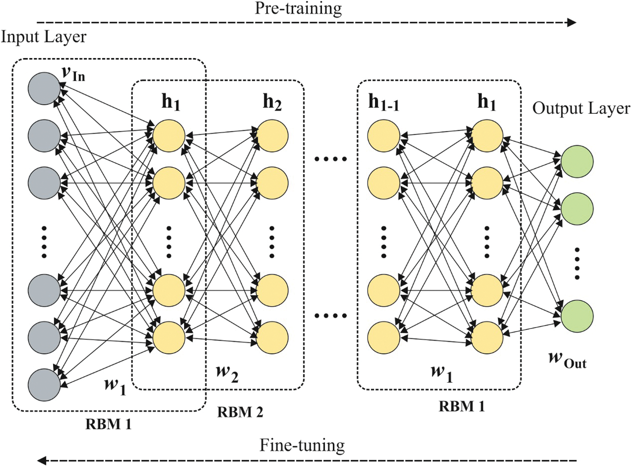
Figure 1: The structure of DBN

While marginal probability distribution of v is illustrated as,

p(v∣θ)=∑hexp⁡(−E(v,h∣θ))∑v,hexp⁡(−E(v,h∣θ))(7)

For gaining best θ value for single data vector v, gradient of log-likelihood evaluation is estimated on the basis of applied expression,

∂logp(v∣θ)∂aj=⟨hj⟩data−⟨hj⟩model,(8)

where ⟨⋅⟩ indicates the expectations by distribution of specific subscript. Due to the absence of links among units in similar layer, ⟨⋅⟩data is simply obtained by measuring the conditional probability distributions and represented as

p(hj∣v,θ)=11+exp⁡(−∑iwijvi−aj)(9)

The activation function is referred as sigmoid function [25]. In case of ⟨⋅⟩model, Contrastive Divergence (CD) learning model is employed by redevelopment to reduce the variations of 2 Kullback–Leibler divergences (KL). Initially, CD learning is effective in real-time application and limits the processing cost when compared with Gibbs sampling approach. Therefore, weights in DBN layers undergo training with the help of unlabeled data by fast and greedy unsupervised mechanism. In case of prediction, supervised layer is included in DBN to change the learned features by using labeled data under the application of up-down fine-tuning method. Here, the Fully Connected (FC) layer acts as a top layer, and sigmoid activation function has been employed.

3.3 Hyperparameter Optimization

In order to fine tune the hyperparameters such as ‘weights’ and ‘bias’ of the DBN model, QBA is employed. It can be extended version of Bat Algorithm (BA). Basically, BA is devised by Yang [26] and evolved from the echolocation features of bats. It is a novel and well-known nature-based metaheuristic technique which is renowned for the capability of integrating the merits of effective models. BA is elegant and effective than Genetic algorithm (GA) and particle swarm optimization (PSO) techniques. A Bat can usually find prey, remove hurdles, and explore food using the advanced echolocation ability and the self-adaptive utility to balance the Doppler Effect in echoes. Traditionally, Doppler Effect and foraging behavior of bats were not considered; instead, it was assumed the bats foraging which is not true and does not resemble the normal performance of bats. In this model, these 2 phenomena were regarded as alternate features of BA. The development of QB in bats expands the foraging nature of bats that contributes to population diversification.

Basically, BA depends upon 3 idealized procedures namely, (1) echolocation capability of bats to predict the distance and to measure the variance among the prey as well as background obstacles, (2) bats change the wavelength (k0) and loudness (A0) for identifying the prey. Moreover, it regulates the frequency as well as rate of the released pulses, which depends upon the distance of prey; (3) assume the loudness has differed from a maximum (A0) value to lower constant value (Amin). The location (xi) and velocities (vi) of virtual bats are upgraded by using the given function:

fi=fmin+(fmax−fmin)α(10)

vit=vit−1+(xit−gt)fi(11)

xit=xit−1+vit(12)

where α,fi,fmin, and fmax indicates the random vector from [0, 1], pulse frequency, lower and higher frequency. Followed by, vit,vit−1,xit,xit−1, and gt means the velocity of ith bat at iteration t, velocity of ith bat at iteration (t−1), and recent optimal global location identified by the bats, correspondingly. The local random walk is applied for generating a novel solution for a bat after selecting a solution from recent optimal solutions. Hence, new position is defined as shown in the following:

xnew=xold+εAt(13)

where ε denotes the arbitrary value from [−1,1] and At indicates the average loudness of bats at iteration t. Thus, optimal solution can be accomplished by the given expressions:

xdt+1=gdt×[1+j(0,σ2)](14)

where j(0,σ2) denotes the Gaussian distribution along with mean 0 and standard deviation (SD)σ2. xdt+1 and gdt implies the location of ith bat at iteration t+1 as well as recent optimal global location examined by bats at dimension d.Ait refers the loudness of ith bat at iteration t. ε means the combined value used to make sure the positive SD σ2. The loudness Ai as well as pulse emission rate ri are upgraded for all iterations by the given functions:

Ait+1=δAit(15)

where Ait, Ait+1, ri0, and rit+1 implies the loudness of ith bat at iteration t, loudness of ith bat at iteration t+1, basic pulse emission rate of ith bat as well as pulse emission rate of ith bat at iteration t+1, correspondingly. d and C resembles constants from [0, 1] and maximum when compared with 0 (γ>0).

In order to make effective performance, maximum number of idealized rules were adopted with 3 idealized rules identified in actual BA namely, (1) Bats are composed of diverse foraging habitats instead of having single foraging habitat which depending upon the stochastic selection and (2) bats are composed of self-adaptive ability to manage the Doppler Effect in echoes [27]. In QBA, quantum-hierarchy virtual bats location is described in the following:

xidt=gdt+β|mbestd−xidt|ln⁡(1u),u(0,1)<0.5(16a)

xidt=gdt−β|mbestd−xidt|ln⁡(1u),u(0,1)≥0.5(16b)

where xidt signifies the location of ith bat in dimension d at iteration t. The bats with self-adaptive management for Doppler Effect modifies the upgrading function as depicted in Eqs. (10) and (11) as follows:

fid=(340+vit−1)(340+vgt−1)×fid×[1+Ci×(gdt−xidt)|gdt−xidt|+ε](17)

vidt=(w×vidt−1)+(gdt−xidt)fid(18)

xidt=xidt−1+vidt(19)

where fid indicates the frequency of ith bat in dimension d; vgt−1 represents the velocity of global best position at iteration t−1, and Ci means the positive value of ith bat within [0, 1]. Then, consider the value of C as 0, afterward bat is unable to compensate the Doppler Effect in echoes and when C= 1, it refers that bat compensates completely for Doppler Effect in echoes. Fig. 2 illustrates the flowchart of BA technique.

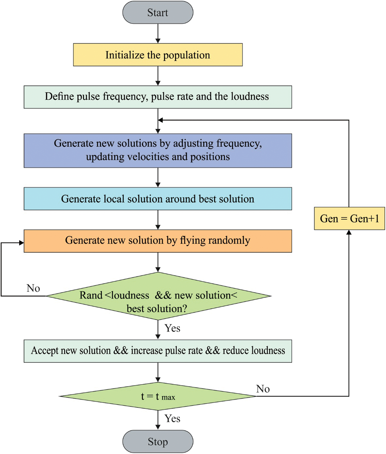
Figure 2: Flowchart of BA algorithm

4  Performance Validation

A detailed experimental analysis of the IDL-STFLP model takes place with other existing techniques interms of precision as shown in Tab. 1 and Fig. 3 under varying volume and speed. The experimental outcome stated that the GNB and KELM models have showcased least precision values whereas the DKELM and DSAE models have portrayed slightly improved precision values. But the presented IDL-STFLP model has resulted in higher precision. For instance, under the volume of 5 min, the IDL-STFLP model has resulted in a maximum precision of 90.783% whereas the other methods such as GNB, KELM, DKELM, and DSAE models have offered a minimum precision of 83.150%, 83.273%, 84.473%, and 85.525%. Likewise, under the volume with 15 min, the IDL-STFLP method has resulted in a higher precision of 94.882% while the alternate methods like GNB, KELM, DKELM, and DSAE models have offered a lower precision of 91.210%, 91.137%, 90.922%, and 91.524%. Similarly, under the volume with 25 min, the IDL-STFLP model has resulted in a maximum precision of 99.275% and the other approaches such as GNB, KELM, DKELM, and DSAE methods have provided a minimum precision of 92.550%, 93.142%, 94.020%, and 93.911%.

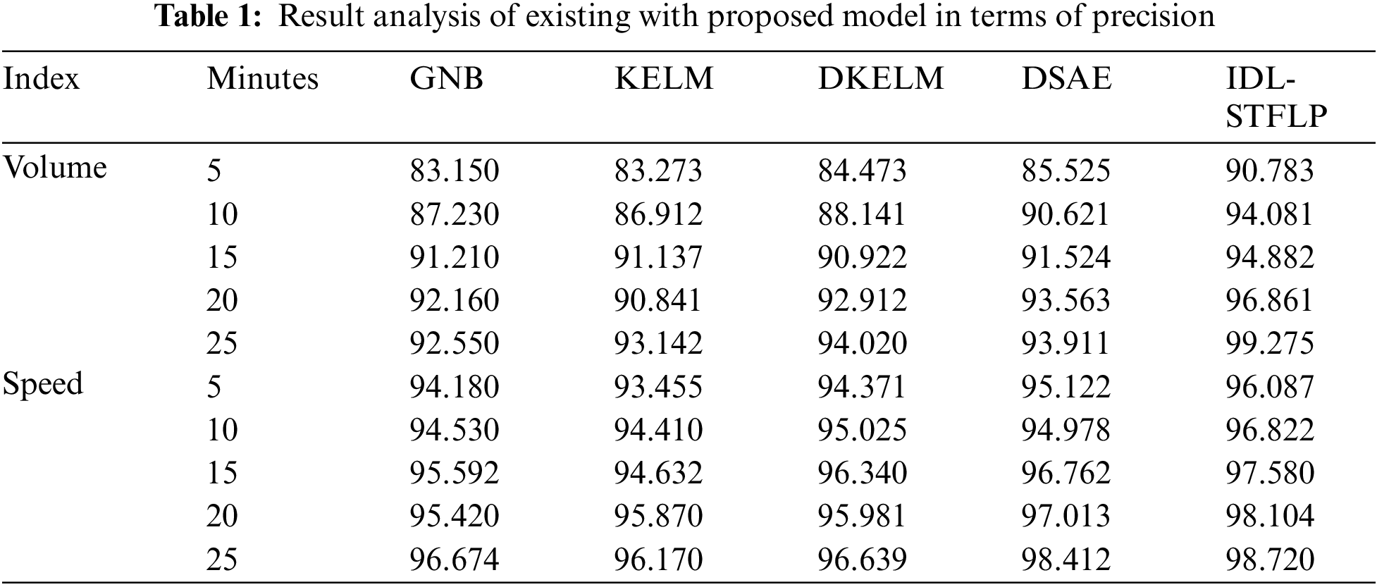
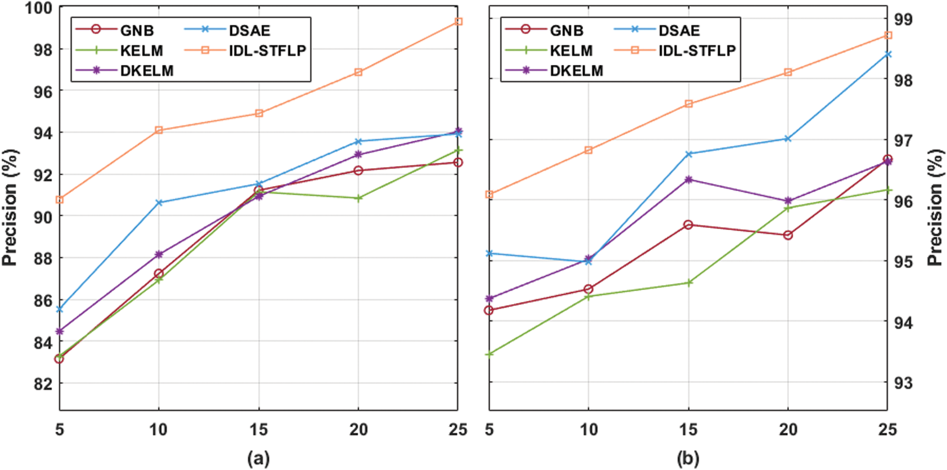
Figure 3: Result analysis of IDL-STFLP model interms of precision (a) Under varying volume, (b) Under varying speed

The experimental results have recommended that the GNB and KELM methods have exhibited minimum precision values while the DKELM and DSAE models have portrayed slightly improved precision values. However, the projected IDL-STFLP scheme has provided maximum precision. For example, under the speed of 5 min, the IDL-STFLP framework has exhibited a maximum precision of 96.087% and alternate methods such as GNB, KELM, DKELM, and DSAE models have displayed least precision of 94.180%, 93.455%, 94.371%, and 95.122%. Likewise, under the speed of 15 min, the IDL-STFLP model has resulted in a maximum precision of 97.580% and the other methods like GNB, KELM, DKELM, and DSAE models have offered a low precision of 95.592%, 94.632%, 96.340%, and 96.762%. Likewise, under the speed of 25 min, the IDL-STFLP model has finalized higher precision of 98.720% while the other methods such as GNB, KELM, DKELM, and DSAE models have offered a minimal precision of 96.674%, 96.170%, 96.639%, and 98.412%.

A detailed experimental examination of the IDL-STFLP model is compared with traditional techniques by means of recall as shown in Tab. 2 and Fig. 4 under varying volume and speed. The experimental results stated that the GNB and KELM models have showcased least recall values whereas the DKELM and DSAE models have depicted slightly improved recall values. But the presented IDL-STFLP model has resulted maximum recall. For instance, under the volume with 5 min, the IDL-STFLP model has shown a maximum recall of 95.310% whereas the other methods such as GNB, KELM, DKELM, and DSAE techniques have offered a minimum recall of 83.020%, 83.890%, 83.530%, and 84.900%. Similarly, under the volume with 15 min, the IDL-STFLP model has resulted in a greater recall of 95.990% whereas the other methods such as GNB, KELM, DKELM, and DSAE models have showcased a minimum recall of 90.840%, 91.060%, 94.410%, and 91.720%. Similarly, under the volume of 25 minutes, the IDL-STFLP model has offered a maximum recall of 98.860% whereas the other methods such as GNB, KELM, DKELM, and DSAE models have exhibited a minimum recall of 92.770%, 93.420%, 96.510%, and 96.460%.

The experimental results stated that the GNB and KELM models have showcased least recall values whereas the DKELM and DSAE models have portrayed slightly improved recall values. But the presented IDL-STFLP model has finalized maximum recall. For instance, under the speed of 5 min, the IDL-STFLP model has resulted in a maximum recall of 96.740% while the other techniques like GNB, KELM, DKELM, and DSAE models have offered a minimum recall of 92.410%, 94.300%, 94.780%, and 96.500%. In line with this, under the speed of 15 min, the IDL-STFLP model has offered a maximum recall of 98.630% whereas the other methods such as GNB, KELM, DKELM, and DSAE models have provided the least recall of 94.570%, 94.590%, 95.120%, and 96.520%. Likewise, under the speed of 25 min, the IDL-STFLP model has showcased higher recall of 99.040% whereas the other methods such as GNB, KELM, DKELM, and DSAE methods have offered a minimum recall of 95.860%, 96.500%, 97.680%, and 97.270%.

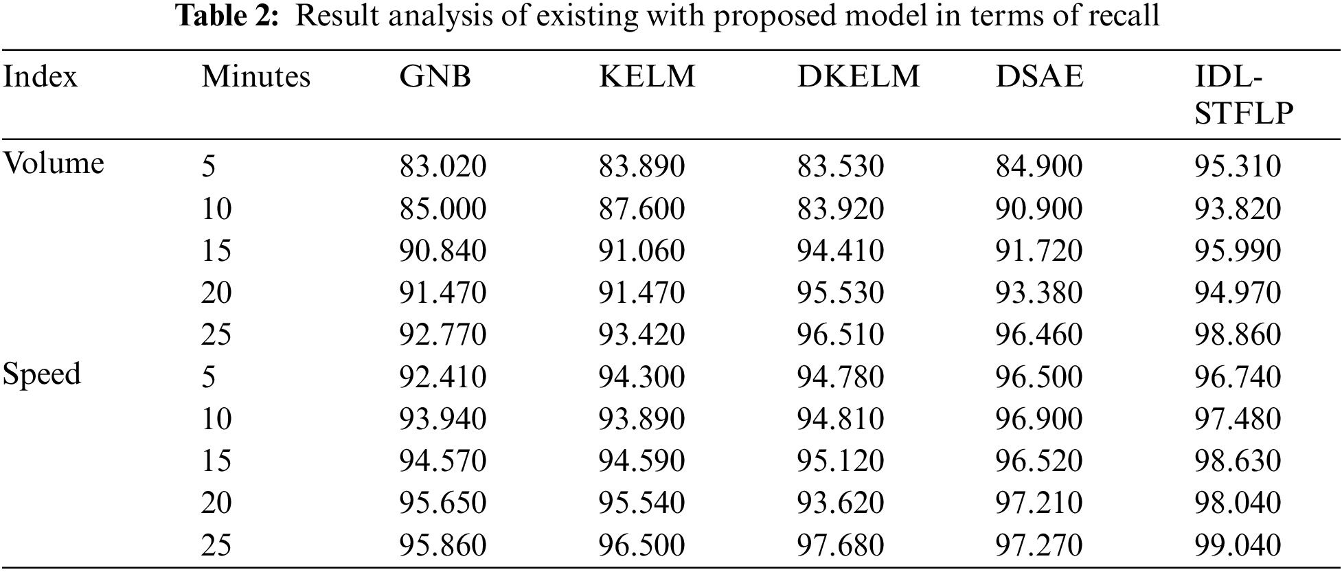
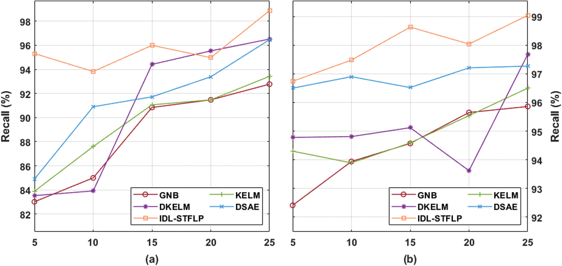
Figure 4: Result analysis of IDL-STFLP model interms of recall (a) Under varying volume, (b) Under varying speed

A detailed experimental analysis of the IDL-STFLP model takes place with other existing techniques with respect to accuracy as depicted in Tab. 3 and Fig. 5 under diverse volume and speed. The experimental results stated that the GNB and KELM models have showcased least accuracy values while the DKELM and DSAE models have portrayed slightly improved accuracy values. Therefore, the proposed IDL-STFLP model has resulted in higher accuracy. For instance, under the volume with 5 min, the IDL-STFLP model has resulted in a maximum accuracy of 92.671% while the other methods such as GNB, KELM, DKELM, and DSAE models have offered a low accuracy of 83.591%, 83.990%, 84.656%, and 84.990%. Similarly, under the volume with 15 min, the IDL-STFLP model has resulted in a maximum accuracy of 94.694% whereas the alternate methods such as GNB, KELM, DKELM, and DSAE models have offered a minimal accuracy of 90.613%, 89.882%, 90.990%, and 91.654%. Likewise, under the volume with 25 min, the IDL-STFLP model has resulted in greater accuracy of 98.411% whereas the other methods such as GNB, KELM, DKELM, and DSAE models have showcased least accuracy of 92.121%, 93.741%, 93.653%, and 94.567%. The experimental outcome depicted that the GNB and KELM models have showcased least accuracy values whereas the DKELM and DSAE models have illustrated slightly improved accuracy values. Then, the proposed IDL-STFLP model has resulted in higher accuracy. For example, under the speed of 5 min, the IDL-STFLP model has offered a maximum accuracy of 96.223% whereas the other methods such as GNB, KELM, DKELM, and DSAE models have offered a lower accuracy of 93.700%, 93.742%, 93.853%, and 95.292%. Likewise, under the speed of 15 min, the IDL-STFLP model has exhibited a maximum accuracy of 98.022% whereas the other models like GNB, KELM, DKELM, and DSAE models have offered a minimum accuracy of 95.450%, 95.222%, 95.457%, and 95.823%. Along with that, under the speed of 25 min, the IDL-STFLP technique has concluded a greater accuracy of 99.210% while the other methods like GNB, KELM, DKELM, and DSAE models have offered a lower accuracy of 96.010%, 95.831%, 95.881%, and 97.997%.

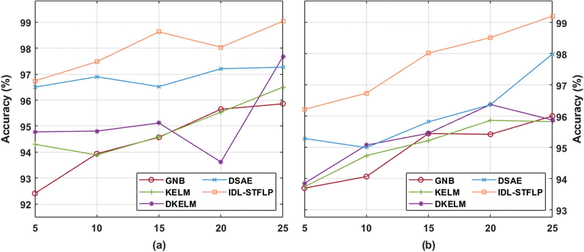
Figure 5: Result analysis of IDL-STFLP model interms of accuracy (a) Under varying volume, (b) Under varying speed

5  Conclusion

This paper has developed an effective IDL-STFLP model for traffic flow prediction in C-ITS. The presented IDL-STFLP model operates on two main stages namely vehicle counting and traffic flow prediction. Primarily, vehicle counting takes place using an FCRC model that carries out the redundant counting rather than the density map prediction to average over errors. Next to the vehicle count process, traffic flow prediction takes place using optimal DBN which has been used for the prediction of traffic flow in short term. A wide range of experimentation analyses was performed and the experimental results denoted that the presented IDL-STFLP method can count vehicles and predict traffic flow in real-time with maximum performance under dissimilar environmental situations. In future, the performance of the IDSL-STFLP model can be raised by the use of advanced deep learning architectures with optimal hyperparameter settings.

Funding Statement: The authors received no specific funding for this study.

Conflicts of Interest: The authors declare that they have no conflicts of interest to report regarding the present study.

References

 1.  M. A. Javed and E. B. Hamida, “On the interrelation of security, QoS, and safety in cooperative ITS,” IEEE Transactions on Intelligent Transportation Systems, vol. 18, no. 7, pp. 1943–1957, 2017. [Google Scholar]

 2.  M. A. Javed, S. Zeadally and E. B. Hamida, “Data analytics for cooperative intelligent transport systems,” Vehicular Communications, vol. 15, no. 7, pp. 63–72, 2019. [Google Scholar]

 3.  T. N. Pham, M.-F. Tsai, D. B. Nguyen, C.-R. Dow and D.-J. Deng, “A cloud-based smart-parking system based on internet-of-things technologies,” IEEE Access, vol. 3, pp. 1581–1591, 2015. [Google Scholar]

 4.  A. S. El-Wakeel, J. Li, A. Noureldin, H. S. Hassanein and N. Zorba, “Towards a practical crowdsensing system for road surface conditions monitoring,” IEEE Internet Things Journal, vol. 5, no. 6, pp. 4672–4685, 2018. [Google Scholar]

 5.  W. Y. H. Adoni, T. Nahhal, B. Aghezzaf and A. Elbyed, “The mapreduce-based approach to improve vehicle controls on big traffic events,” in 2017 Int. Colloquium on Logistics and Supply Chain Management, Rabat, Morocco, pp. 1–6, 2017. [Google Scholar]

 6.  G. Guerreiro, P. Figueiras, R. Silva, R. Costa and R. J. Goncalves, “An architecture for big data processing on intelligent transportation systems. An application scenario on highway traffic flows,” in 2016 IEEE 8th Int. Conf. on Intelligent Systems, Sofia, Bulgaria, pp. 65–72, 2016. [Google Scholar]

 7.  Q. Meng, H. Song, Y. Zhang, X. Zhang, G. Li et al., “Video-based vehicle counting for expressway: A novel approach based on vehicle detection and correlation-matched tracking using image data from ptz cameras,” Mathematical Problems in Engineering, vol. 2020, pp. 1–16, 2020. [Google Scholar]

 8.  Y. Xiang, A. Alahi and S. Savarese, “Learning to track: Online multi-object tracking by decision making,” in Proc. of the Computer Vision, Santiago, Chile, pp. 4705–4713, 2015. [Google Scholar]

 9.  M. S. Dougherty and M. R. Cobbett, “Short-term inter-urban traffic forecasts using neural networks,” International Journal of Forecasting, vol. 13, no. 1, pp. 21–31, 1997. [Google Scholar]

10. H. R. Kirby, S. M. Watson and M. S. Dougherty, “Should we use neural networks or statistical models for short-term motorway traffic forecasting?,” International Journal of Forecasting, vol. 13, no. 1, pp.43–50, 1997. [Google Scholar]

11. H. Dia, “An object-oriented neural network approach to short-term traffic forecasting,” European Journal of Operational Research, vol. 131, no. 2, pp. 253–261, 2001. [Google Scholar]

12. J. Wang and Q. Shi, “Short-term traffic speed forecasting hybrid model based on chaos-wavelet analysis-support vector machine theory,” Transportation Research Part C: Emerging Technologies, vol. 27, no. 92, pp. 219–232, 2013. [Google Scholar]

13. P. V. V. K. Theja and L. Vanajakshi, “Short term prediction of traffic parameters using support vector machines technique,” in 2010 3rd Int. Conf. on Emerging Trends in Engineering and Technology, Goa, India, pp. 70–75, 2010. [Google Scholar]

14. B. Çetiner, M. Sari and O. Borat, “A neural network based traffic-flow prediction model,” Mathematical and Computational Applications, vol. 15, no. 2, pp. 269–278, 2010. [Google Scholar]

15. K. Kumar, M. Parida and V. K. Katiyar, “Short term traffic flow prediction in heterogeneous condition using artificial neural network,” Transport, vol. 30, no. 4, pp. 397–405, 2015. [Google Scholar]

16. J. Guo, W. Huang and B. M. Williams, “Adaptive kalman filter approach for stochastic short-term traffic flow rate prediction and uncertainty quantification,” Transportation Research Part C: Emerging Technologies, vol. 43, no. 2, pp. 50–64, 2014. [Google Scholar]

17. F. G. Habtemichael and M. Cetin, “Short-term traffic flow rate forecasting based on identifying similar traffic patterns,” Transportation Research Part C: Emerging Technologies, vol. 66, pp. 61–78, 2016. [Google Scholar]

18. M. Ma, S. Liang, H. Guo and J. Yang, “Short-term traffic flow prediction using a self-adaptive two-dimensional forecasting method,” Advances in Mechanical Engineering, vol. 9, no. 8, pp. 16–12, 2017. [Google Scholar]

19. J. Guo, Z. Liu, W. Huang, Y. Wei and J. Cao, “Short-term traffic flow prediction using fuzzy information granulation approach under different time intervals,” IET Intelligent Transport Systems, vol. 12, no. 2, pp. 143–150, 2018. [Google Scholar]

20. J. P. Cohen, G. Boucher, C. A. Glastonbury, H. Z. Lo and Y. Bengio, “Count-ception: Counting by fully convolutional redundant counting,” in 2017 IEEE Int. Conf. on Computer Vision Workshops, Venice, pp. 18–26, 2017. [Google Scholar]

21. G. N. Nguyen, N. H. L. Viet, M. Elhoseny, K. Shankar, B. B. Gupta et al., “Secure blockchain enabled cyber-physical systems in healthcare using deep belief network with ResNet model,” Journal of Parallel and Distributed Computing, vol. 153, no. 2, pp. 150–160, 2021. [Google Scholar]

22. I. V. Pustokhina, D. A. Pustokhin, J. J. P. C. Rodrigues, D. Gupta, A. Khanna et al., “Automatic vehicle license plate recognition using optimal k-means with convolutional neural network for intelligent transportation systems,” IEEE Access, vol. 8, pp. 92907–92917, 2020. [Google Scholar]

23. N. Metawa, I. V. Pustokhina, D. A. Pustokhin, K. Shankar, M. Elhoseny et al., “Computational intelligence-based financial crisis prediction model using feature subset selection with optimal deep belief network,” Big Data, vol. 9, no. 2, pp. 100–115, 2021. [Google Scholar]

24. J. Yu and G. Liu, “Knowledge-based deep belief network for machining roughness prediction and knowledge discovery,” Computers in Industry, vol. 121, no. 4, pp. 103262, 2020. [Google Scholar]

25. Y. Jia, J. Wu and M. Xu, “Traffic flow prediction with rainfall impact using a deep learning method,” Journal of Advanced Transportation, vol. 2017, no. 722, pp. 1–10, 2017. [Google Scholar]

26. P. Progias, A. A. Amanatiadis, W. Spataro, G. A. Trunfio and G. Ch Sirakoulis, “A cellular automata based FPGA realization of a new metaheuristic bat-inspired algorithm,” AIP Conference Proceedings, vol. 1776, no. 1, pp. 800002, 2016. [Google Scholar]

27. F. P. Mahdi, P. Vasant, M. A. A. Wadud, V. Kallimani and J. Watada, “Quantum-behaved bat algorithm for many-objective combined economic emission dispatch problem using cubic criterion function,” Neural Computing and Applications, vol. 31, no. 10, pp. 5857–5869, 2019. [Google Scholar]

This work is licensed under a Creative Commons Attribution 4.0 International License, which permits unrestricted use, distribution, and reproduction in any medium, provided the original work is properly cited.