DOI:10.32604/cmc.2022.021410
| Computers, Materials & Continua DOI:10.32604/cmc.2022.021410 | |
| Article |
Weighted-adaptive Inertia Strategy for Multi-objective Scheduling in Multi-clouds
1Department of Communication Technology and Networks, Universiti Putra Malaysia (UPM), Serdang, 43400, Malaysia
2Institute for Mathematical Research (INSPEM), Universiti Putra Malaysia (UPM), Serdang, 43400, Malaysia
3Faculty of Education-Saber, University of Aden, Aden, 2408, Yemen
*Corresponding Author: Mazen Farid. Email: mazenfareed7@yahoo.com
Received: 02 July 2021; Accepted: 11 October 2021
Abstract: One of the fundamental problems associated with scheduling workflows on virtual machines in a multi-cloud environment is how to find a near-optimum permutation. The workflow scheduling involves assigning independent computational jobs with conflicting objectives to a set of virtual machines. Most optimization methods for solving non-deterministic polynomial-time hardness (NP-hard) problems deploy multi-objective algorithms. As such, Pareto dominance is one of the most efficient criteria for determining the best solutions within the Pareto front. However, the main drawback of this method is that it requires a reasonably long time to provide an optimum solution. In this paper, a new multi-objective minimum weight algorithm is used to derive the Pareto front. The conflicting objectives considered are reliability, cost, resource utilization, risk probability and makespan. Because multi-objective algorithms select a number of permutations with an optimal trade-off between conflicting objectives, we propose a new decision-making approach named the minimum weight optimization (MWO). MWO produces alternative weight to determine the inertia weight by using an adaptive strategy to provide an appropriate alternative for all optimal solutions. This way, consumers’ needs and service providers’ interests are taken into account. Using standard scientific workflows with conflicting objectives, we compare our proposed multi-objective scheduling algorithm using minimum weigh optimization (MOS-MWO) with multi-objective scheduling algorithm (MOS). Results show that MOS-MWO outperforms MOS in term of QoS satisfaction rate.
Keywords: Multi-cloud environment; multi-objective optimization; Pareto optimization; workflow scheduling
The cloud environment provides a platform where servers in a data center can be accessed in shared mode when users request services [1]. Cloud computing architecture is composed of three distinct layers, namely Infrastructure as a Service (IaaS), Software as a Service (SaaS) and Platform as a Service (PaaS). SaaS integrates three different organizations: cloud providers, software providers and users. A multi-cloud system involves the collaboration of multiple cloud infrastructure providers (such as Microsoft Azure, 2018; Amazon EC2, 2018 and Google Compute Engine, 2018) that configure their computing needs using a wide range of cloud-based IaaS. They provide their virtual machines at a price using “pay as you go” models which is one of the most popular ways to share resources between cloud providers. [2,3].
The workflow is a common method for modeling most distributed systems used in scientific applications. It is typically represented as an acyclic graph where the relation between tasks is shown on the edges of each node. Usually, the number of tasks is greater than the number of virtual machines (VMs) available. This necessitates the use of an appropriate scheduling policy for task assignments. Recently, workflow scheduling in the cloud has been a subject of focus due to the importance of workflow applications. Therefore, selecting the near-optimal schedules in such scenarios is generally NP-hard.
Most of the recently proposed solutions have only taken one of the qualities of service (QoS) requirements into account. For example, the workflow completion time is considered when investigating makespan. Other important factors related to QoS include cost, cloud security, performance and reliability. Hence, an efficient task scheduling algorithm must strike a balance between several QoS objectives. This is known as multi-objective task scheduling. One way of striking such a balance is the use of Pareto optimal algorithms that allow users to select the best result within an acceptable set of solutions.
A Pareto optimal solution simultaneously optimizes conflicting objectives. If the optimal solution has a number of candidates, the set is known as the Pareto front. No solution is considered dominant within the Pareto front. Since heuristic algorithms are generated, it becomes difficult to choose the appropriate permutation for service providers [4]. The main drawback of the Pareto optimization method is that it needs a longer time to make a better final decision [5]. The authors of [6] used a well-known decision-making process called weighted aggregated sum product assessment (WASPAS). This method enables service providers to communicate their needs and give specific weight to objectives based on consumers’ preferences. It selects the best solution from the optimal Pareto set with respect to a given priority.
In this article, we propose a multi-objective workflow scheduling algorithm with minimum weight optimization (MWO) method. A Pareto front is used to reveal all possible solutions and determine an optimal solution. This way, both the service provider and customer needs can be catered for simultaneously. The introduced algorithm utilizes the MWO method to meet the following five requirements.
1. Minimum workflow time (makespan).
2. Minimum cost.
3. Maximum resources utilization.
4. Maximum workflow reliability.
5. Minimum risk probability of workflow.
In real-time applications, some users may be concerned with makespan reduction, some other users may care about the cost of paying VMs while others focus on high workflow reliability. In contrast to these users’ concerns, VM providers aim at maximizing the utilization of their resources and minimizing risk probability. Therefore, a multi-objective method of optimization is needed to achieve an almost optimum trade-off between these conflicting concerns and satisfy them simultaneously.
In this article, the main contributions are:
1. Presenting a multi-objective method for scheduling workflow in a cloud environment based on the particle swarm optimization (PSO) algorithm.
2. Defining a fitness function that simultaneously considers the interests of users and service providers (by decreasing makespan, cost and risk probability and increasing resource utilization and reliability).
3. Deploying a newly proposed decision-making method called minimum weight optimization to choose a feasible solution and illustrating the solution using the Pareto front based on users’ preferences.
4. Using alternative weight values to determine the inertia weight by deploying an adaptive strategy to increase the convergence of the PSO in the first few iterations of the algorithm.
The rest of this paper is organized thus: Section 2 presents an overview of the related works. Section 3 defines the scheduling model and explains the problem and network model formulation. Section 4 discusses the multi-objective optimization methods. Section 5 presents the proposed algorithm and details its implementation while Section 6 elaborates the experimental setup and simulation results. Section 7 discusses the performance measurement and Section 8 concludes this article.
Finding the most suitable workflow scheduling solution is an NP-hard problem. A workflow scheduling method is generally aimed at achieving one specific or multiple objectives. It balances the trade-off between conflicting objectives. One of such multi-objective scheduling methods is the aggregation method. This strategy tackles a multi-objective scheduling problem by converting it to a single objective. The weight is taken into account for each objective and the number of weighted objectives is optimized. In [7], a multi-objective problem was transformed into a single objective problem using cost-conscious scheduling. The system was designed to maximize makespan and minimize cost. Jeannot et al. [8] proposed a scheduling strategy that increases performance and reliability using the aggregation method. During runtime, the dynamic level strategy (DLS) introduced in [9], can changes the task priority. Doǧan et al. [10] enhanced the DLS method with a genetic algorithm and proposed Bi-objective Dynamic Level Scheduling (BDLS).
The Pareto approach differs from the aggregation approach as it leads to a trade-off between undesired objectives that should be reduced (e.g., cost) and desired objectives that should be maximized. Such algorithms are assisted by solutions that are non-dominant in the Pareto front. Adopting this approach, Sagnika et al. [11] introduced a Cat Swarm Improvement algorithm to schedule workflows in the cloud. The algorithm reduces the time consumption, cost and processor's idle time. The authors compared the proposed method with multi-objective particle swarm optimization (MOPSO) algorithm and the results revealed that the proposed algorithm performs better than MOPSO.
A multi-objective scheduling method was proposed by Udomkasemsub et al. [12] using the Pareto optimizer algorithm with the Artificial Bee Colony (ABC) algorithm to minimize cost and makespan. Similarly, Wu et al. [13] proposed an RDPSO algorithm for managing workflows in the cloud to reduce cost or makespan. In [14], a new multi-objective scheduling approach that uses the Gray Wolf algorithm was introduced with a focus on cost, makespan and resource efficiency. Another multi-objective approach using the MODPSO algorithm was proposed by Yassa et al. [15] to reduce cost, energy and makespan. Dynamic voltage and frequency scaling was used to minimize cost. The proposed scheduling algorithm was compared with the Heterogeneous Earliest Finish Time (HEFT) algorithm.
Considering more than two significant scheduling factors, [16] deployed a heuristic black hole multi-objective Pareto-based algorithm. They proposed a suitable approach for analyzing the problem of cloud scheduling to reduce cost and makespan and increase resource efficiency. Kaur et al. [17] proposed an incremented frog slipping algorithm for scheduling workflows to reduce the execution cost while meeting the task deadline. Simulation, using WorkflowSim, reveals that the proposed scheme outperforms the PSO-based approach with respect to minimizing the overall workflow execution cost. Khalili et al. [14] focused on preserving the QoS requirement for service providers by developing a multi-objective scheduling algorithm using the Grey Wolf and Pareto optimizers to decrease makespan, time and cost. The algorithm increases throughput, which is a fundamental service requirement, compared to the Strength Pareto Evolutionary Algorithm 2 (SPEA2).
An adaptive multi-objective scheduling method for mapping workflow at the IaaS level was proposed by Zhang et al. [18]. Their goals are to reduce user resource costs and balance loads on VMs without violating the deadline constraint of the workflow. The Non-dominated Sorting Genetic Algorithm-2 (NSGA2) extension, which uses mutation and crossover operators, was used to achieve Pareto-front and search diversity. The authors deployed Inverted Generational Distance (IGD) which measures the minimum Euclidean distance and calculated the diversity and convergence of a collection of Pareto solutions. In an attempt to reduce costs, makespan time and the use of cloud energy related to the workload deadline, a new approach to workflow scheduling was suggested by Singh et al. [19]. The authors grouped users using machine learning technology. Thereafter, time, cost and negotiation-based policies were considered. Simulation results from CloudSim indicated that the proposed strategy is consistent with other methods in relation to the three objectives studied.
Verma et al. [20] proposed Hybrid PSO (HPSO) by incorporating budget and deadline constrained heterogeneous earliest finish time algorithm (BDHEFT) to schedule multi-objective workflows with budget and deadline constraints. MOPSO is used to reduce resources cost and workflow makespan during the scheduling process. The original solution can be generated through BDHEFT and other randomly selected initial solutions. During the MOPSO implementation cycle, optimal (non-dominated) solutions are maintained as the Pareto front. The final solution is the ultimate Pareto set. Dharwadkar et al. [21] introduced a new programming method, called Horizontal Reduction (HR), to minimize failure, execution costs, scheduling overhead and makespan by integrating control point, replication and PTE algorithms. The findings revealed that the suggested approach outperforms other methods in terms of the three objectives studied.
In [16], a new multi-objective hyper-volume algorithm that expands the black hole detection algorithm was proposed. The algorithm uses a dominant strategy that increases its flexibility and convergence towards the Pareto optimum. The conflicting objectives optimized are resource utilization, resource cost and makespan (completion time). Durillo et al. [22] presented a list-based multi-objective workflow scheduling algorithm. A single-objective Pareto optimizer was used to minimize the resource utilization cost and makespan. Another new multi-objective scheduling approach called Multi-objective HEFT (MOHEFT) [22] was also presented. [23] further proposed an improvement of [24], called the Pareto Multi-objective List Scheduling Heuristic (PMLSH), for estimating solutions when ranking in HEFT. A consistency metric, Crowding Distance (CD), was deployed to maximize various objectives. CD is a test to assess the solutions around a particular population of solutions. In each iteration of the algorithm, one can choose nearer optimal solutions. Hypervolume was used as a benchmark to test the proposed algorithm.
Yu et al. [25] used a multi-objective evolutionary algorithm (MOEA) to solve issues regarding workflow planning. The strategy was applied to reduce two conflicting issues which are the costs of utilizing services and the time of implementation. In addition to that, they established objective functions that are compatible with the constraints. Similarly, Kalra et al. [26] put forth a workflow scheduling method by integrating Intelligent Water Drop and Genetic Algorithms (IWD-GA). The method reduces makespan and execution cost and offered a variety of solutions with respect to reliability and deadline constraints. IWD-GA helped consumers to flexibly select solutions based on their requirements.
From the above, it is clear that multi-objective workflow scheduling algorithms take many objectives into consideration to provide effective scheduling. In this regard, an accurate selection (of objectives) is required to effectively allocate tasks to the virtual machines. Most of the previous studies in related literature used Pareto optimality approach [14,26]. However, increasing the number of conflicting objectives increases the Pareto computation cost and completion time. Other methods like aggregation and hypervolume are not scalable when the number of objectives are increased [8,16]. In order to address these limitations, we develop the minimum weight approach that reduces the cost and time of the scheduling process and improves the scalability even with a higher number of objectives. Thus, this paper introduces a new multi-objective scheduling minimum weight optimization (MOS-MWO) algorithm for scheduling scientific workflow in a multi-cloud environment using the MWO process. This is targeted at reducing workflow costs, risk probability and makespan and increasing reliability and resource utilization within the set reliability constraints.
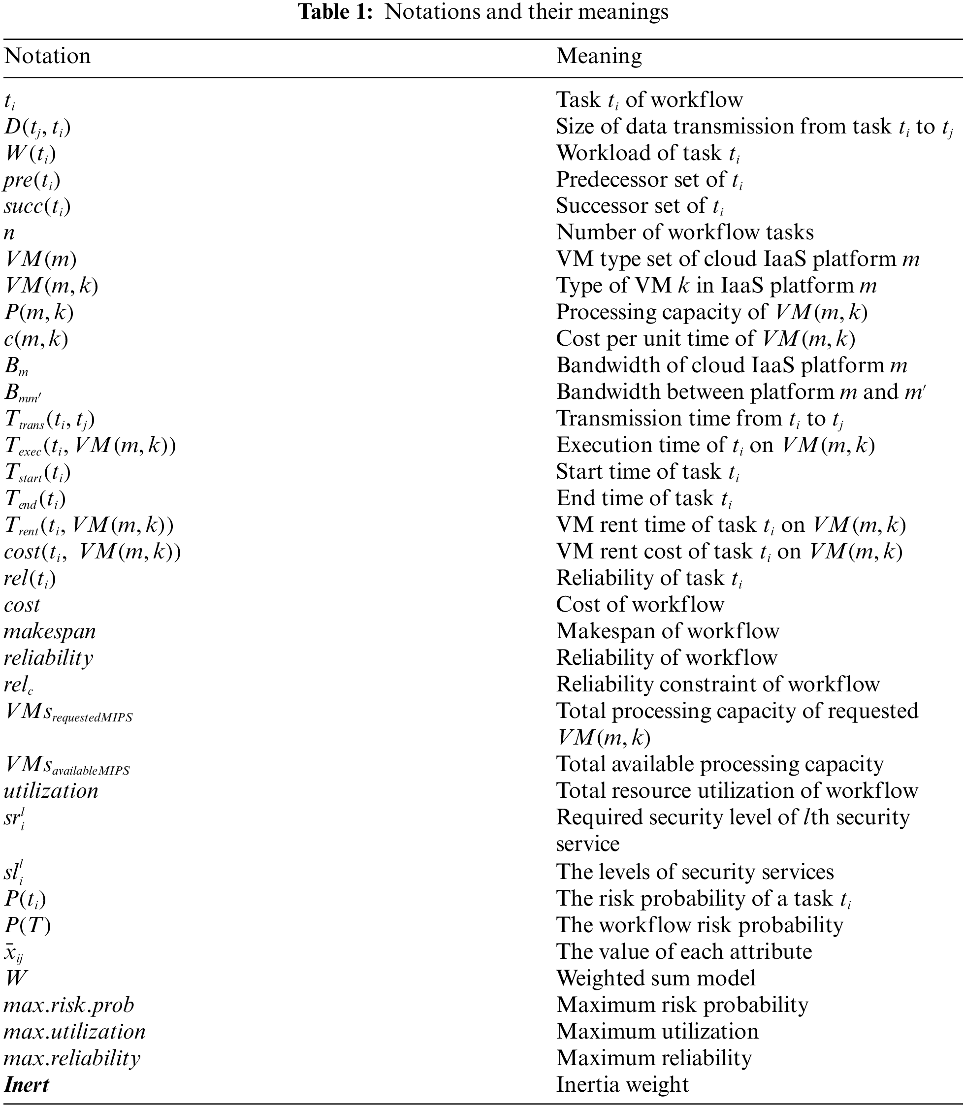
This section discusses the workflow scheduling model and metrics with special attention to reliability, makespan, cost, workflow model, multi-cloud model, resource utilization, risk probability and problem formulation. The proposed MOS-MWO algorithm considers five QoS requirements: cost, risk probability, makespan, resource utilization and reliability. The schedule model is provided in Fig. 1 while the notations used in this study are defined in Tab. 1.

Figure 1: Scheduling model
The first phase involves designing the cloud user workflow application structure. Workflows are distributed to a suitable cloud infrastructure that meets workflow requirements and VM types. Each cloud provider has a task queue and these tasks are executed according to the workflow structure. Since cloud users have access to an infinite number of VM resources, simultaneous services are provided for concurrent tasks based on dependence relationships. It is vital to know that every cloud service provider has its own performance and price trends in the multi-cloud environment.
A sequence of scheduled activities is necessary to achieve a defined objective. These activities are known as workflows. Workflows provide sets of basic processes designed to address a more complicated problem [27]. These processes must follow a standard pattern to ensure coherence and to improve the efficiency of executing the desired tasks. A workflow aims to decide how various tasks can be configured, performed and monitored.
Workflow can be modeled with nodes and edges as a direct acyclic graph (DAG). It can be expressed as W = (T, E), where the task set consists of T = {t0, t1,…, ti,…, tn − 1}. A number of arcs E = {(ti, tj)|ti, tj
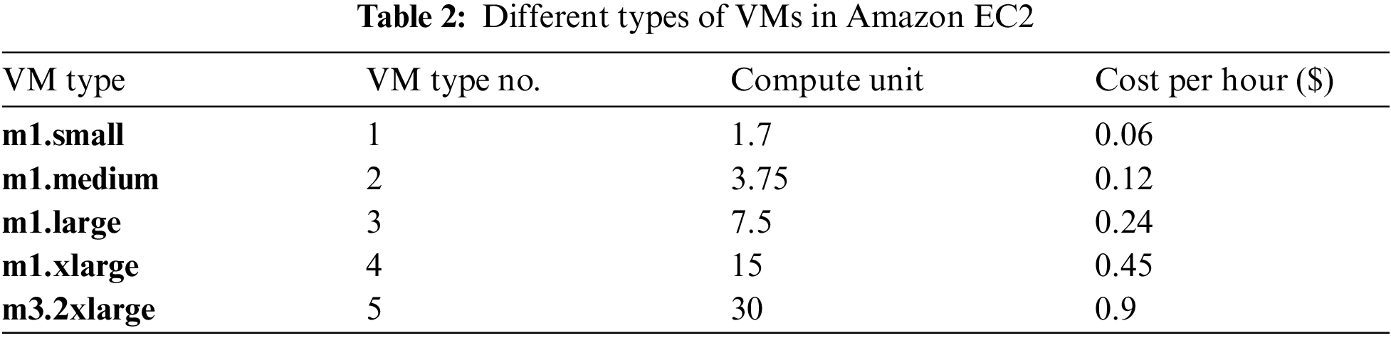
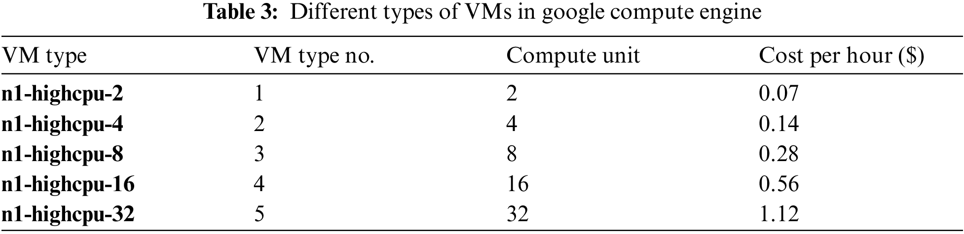
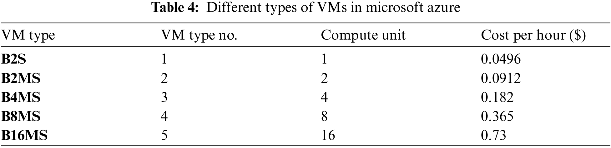
This paper considers three providers of cloud services: Google Compute Engine, Amazon EC2 and Microsoft Azure. Here, we discuss the multi-cloud architecture that gives users access to VMs from multiple cloud providers with different pricing models. For example, (Amazon EC2, 2018) rate is based on operating hours. Every partial clock gradually hits full hours. Likewise, (Azure, 2018) consumers pay per minute. (Google Compute Engine, 2018) charges per minute after the first ten minutes the VM instances are launched. The various types of VMs are shown in Tabs. 2–4.
Different IaaS platforms can be provided in a multi-cloud environment for a collection of VMs where VM(m) = {VM(m, 1),…,VM(m, k),…, VM(m, ks)}, m = 1, 2,…,M. Let (m|m = 1, 2 and 3), where m represents various IaaS cloud providers (i.e., Amazon, Microsoft and Google). The VM(m, k) is the instance VM specified by the IaaS cloud provider m. P(m, k) is its processing power, hourly costs are denoted by C(m, k) and CU refers to the VM CPU computing capacity [28–30]. We assume the various cloud providers can supply end users with an unlimited number of VMs. Bm indicates the bandwidth of cloud platform m and Bmm’ is a bandwidth between two cloud platforms m and m’.
In a multi-cloud environment, workflow/tasks on various IaaS platforms can be delegated and executed. Other VMs need to wait before tasks are received. This is because VMs transfer many copies of their output to other VMs. The nature of the receiver's performance depends on the task order. Eq. (1) defines the group sorting process of workflow/tasks in set A.
The sequence of the tasks in partial set B is the same as the previous tasks ti in A. If A = {t1, t3, t4, t2}, then B = {t1, t3} if ti = t4. The start time of the task ti is represented as Tstart(ti) in Eq. (2) and the end time is Tend(ti).
where Twait(tj, ti) is the waiting time for ti to receive input data from task tj. This is presented as follows:
Note that if ti = tentry, then Tstart(ti) = 0.
In order to calculate the transmission time, we have
where the transmission time between ti and tj is Ttrans(tj, ti).
As a result, task ti has a receiving time given by
The time of execution of each task ti depends on the output data size for each task [31,28]. The execution time to perform different tasks on a different VM(m, k) can be determined using the following equation.
The processing capacity of VM(m, k) in CU can be taken for the end time of each task. Therefore,
Then,
Makespan is the last task's end time
IaaS platforms have unique pricing methods that follow the multi-cloud model. The existing workflow algorithms compute the rental time of the VM by taking the interval from start time to finish time [28,30–32]. When the task is done, the VM stops and the task output is transferred to its successor. Data transfer priority depends on the task order. The time of sending task ti can be specified as:
The rental time of the task ti for the VM running on VM(m, k) is specified in Eq. (11).
The VM rental cost for task ti on each IaaS platform is calculated below.
For Amazon EC2 which charges per hour, task ti cost on VM(1, k) is expressed in Eq. (12).
where Tminute = 60.
Microsoft Azure charges per minute, task ti execution cost on VM(2, k) is stated in Eq. (13).
Google charges the instance per minute after the first ten minutes. This is indicated as the task cost on VM(3, k) in Eq. (14), where Tten = 10.
The cost of the workflow can be calculated using Eq. (15).
The budget constraint can be calculated during workflow scheduling using VMs with the maximum price in a critical path.
3.5 Resource Utilization Computation
Scheduling plays a crucial role in efficiently allocating resources for cloud operation. Many scheduling processes are also conducted by assigning tasks to strike a balance between cost-effectiveness, resource utilization and makespan [33]. It takes more time for cheaper resources to complete task execution than expensive ones. This means that a VM's CPU achieves better resource efficiency at the expense of cost. The total capacity of a requested VM is calculated in Eq. (16).
The workflow utilization percentage for each workflow can be determined using Eq. (17).
Since users always assume that they are working with a service provider that provides high resource utilization, the value of max.utilization is set to 100 in Eq. (32).
Cloud computing failures are unavoidable. Failures may result from within (for example, software faults, hardware failures, power defects, etc.) [34,35] or outside (for example, harmful web attacks) [36,37]. Short-term failures also occur thereby causing failure during task workflow. The case of failure can be based on the Poisson distribution [8,38,39]. It is determined by computing the exponential of the reliability that task
where the cloud service provider failure coefficient λm > 0 (m = 1, 2, 3).
Every IaaS platform also has a specific multi-cloud failure coefficient. If there are problems during the rental period, the mission may fail. So long as the failures are independent, the reliability of the workflow is determined by Eq. (19).
Suppose λmax = max{ λm|m = 1, 2, 3} indicates the maximum failure coefficient and λmin = min{ λm|m = 1, 2, 3} refers to the minimum failure coefficient, the resulting scheduling workflow for the reliability can be Maximum (relmax) or Minimum (relmin). In addition, different workflow results are generated in different clouds according to the task scheduling process. Consequently, cloud users must set appropriate reliability constraint relc for the scientific workflow application, i.e., relc ∈ [relmin, relmax].
Workflow applications are run in a non-risk-free cloud computing environment and thus, security awareness is critical for quantitative assessment of services. The risk analysis model determines the risk rate throughout the workflow [36]. The model assumes that the probability of risks is determined by the level of security and that the distribution of the risk for any fixed interval is based on the Poisson probability distribution. The risk probability of the security service lth for the task can therefore be defined by an exponential distribution as follows [40,41]:
a, g and c represent the services of authentication, integrity and confidentiality, respectively.
Three major cloud threats are snooping, altering and spoofing, and the three security services used to secure scientific workflow applications are authentication service, integrity service and confidentiality service [42]. Users flexibly merge these security services to provide a robust defense against different risks and attacks. The designed model assumes that a typical task will involve three types of security services with different user-defined security rates. For example,
The risk coefficient
The workflow risk probability P(T) with task set T can be calculated according to Eq. (22).
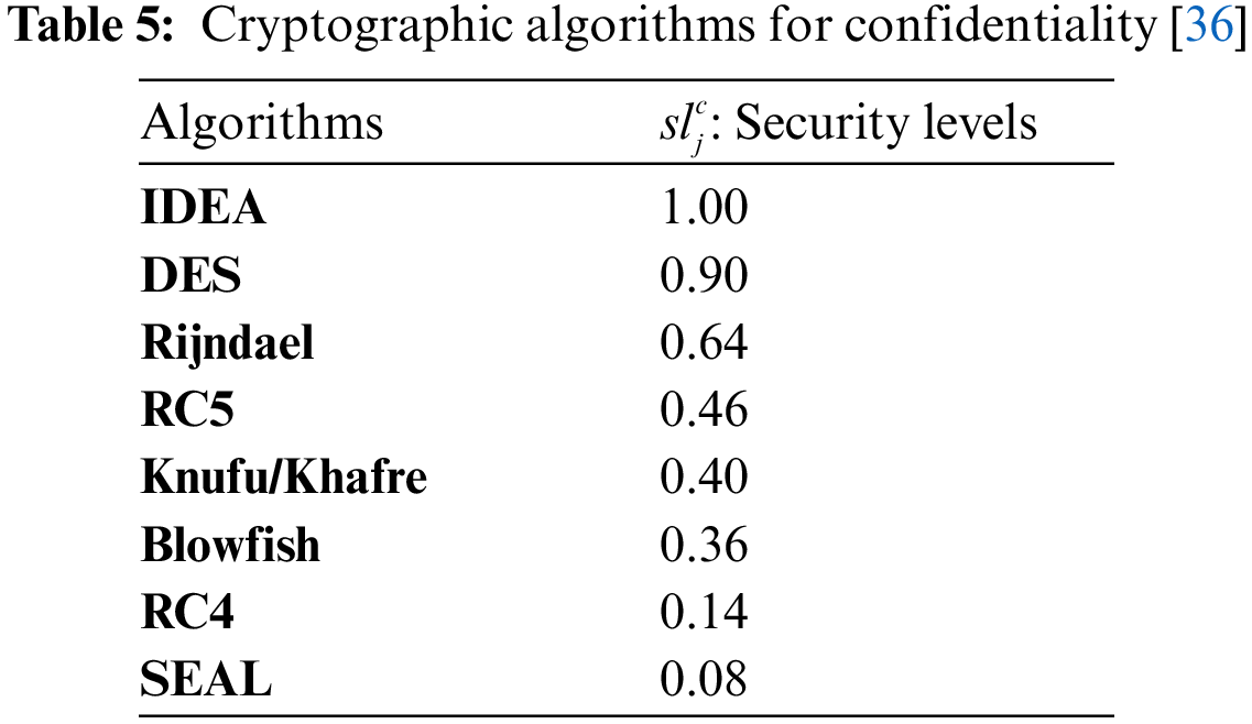
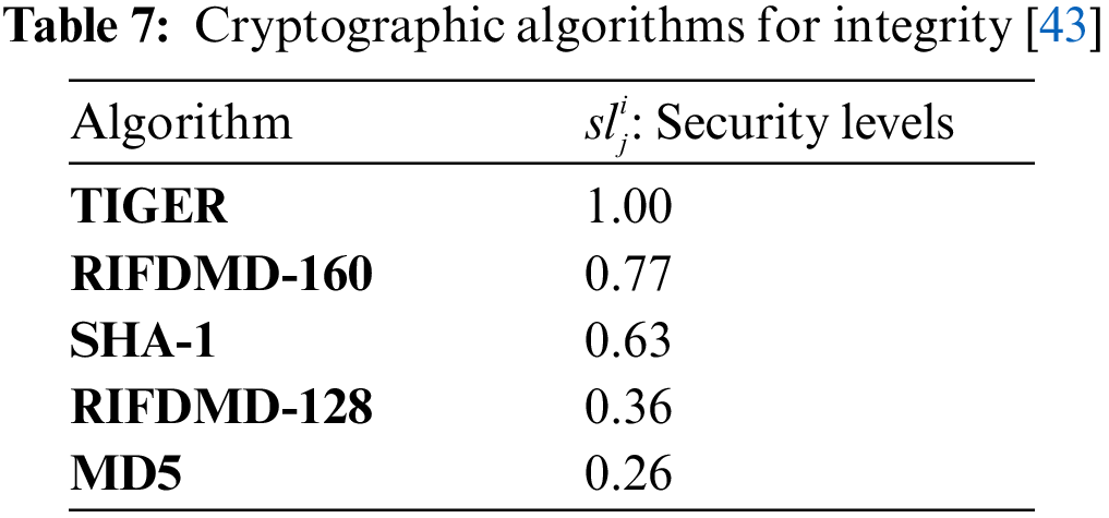
This workflow risk probability will be used as a QoS constraint for problem formulation in the next section. The confidentiality, availability and integrity algorithms are shown in Tabs. 5–7 [36,42,43]. Based on the cryptographic algorithm efficiency, a security level of 0.08 to 1 is assigned to each algorithm. Let the set

For each objective, there is a corresponding user-defined scheduling requirement. The constraint is referred to as a hard requirement. Most of the previous studies [2,44] used the deadline constraint as the user-defined hard requirement. But in our experiments, we determined the deadline as the completion time of the workflow scheduling process using a critical path with the lowest processing capacity of VMs.
Budget constraint is another user-defined hard requirement. Budget is determined in our experiments as the maximum cost of the critical path for scheduling workflow using VMs with the most expensive price.
The probability that task ti will be performed correctly on any VM is calculated using the exponential distribution as shown in Eq. (18). According to Eq. (19), the reliability of the workflow is calculated as the product of task reliabilities. Thus, workflow reliability becomes smaller. For this reason, we use the mean reliability of each workflow to get the workflow total reliability as shown below.
Since users always assume that they are working with a service provider that provides high resource utilization and high reliability, the value of max.utilization and max_reliability are set to 100 in Eq. (32).
The focus of this paper is to maximize resource utilization and reliability and reduce risk probability, makespan and cost. Thus, the workflow is represented as WF = (T, E). The primary objective is scheduling Γ = (Loc, Ord, R), where Loc = {loc(t0), loc(t1),…, loc(tn − 1)} is the workflow task to be executed, Ord = {ord(t0), ord(t1),…, ord(tn − 1)} is the task's data transfer order used primarily to determine the tasks waiting time (the tasks order must also reflect dependence relations), R = {R0, R1,…, Ri,…, Rn − 1} is a set of resources for the whole workflow where Ri = (ti, VM(m; k), Tstart (ti), Tend(ti)). Next, we formally describe the multi-objective optimization problem.
Some previous studies have designed scheduling methods for task execution [28,31,36] but the data transmission order has not been prioritized. Meanwhile, this is particularly important in the design of a scheduling strategy. The scheduling results would be different if different tasks are executed in the same location. We, therefore, take into account the priority of data transmission.
4 Multi-Objective Optimization Methods
In this section, two algorithms (MOS [45] and MOS-MWO) by which the Pareto frontier set can be derived are discussed. Similarly, the effectiveness of these multi-objective optimization methods is compared. According to [46], the Pareto optimal solutions must be preferably accurate and uniformly distributed. Thus, three common effectiveness metrics (distance distribution, coverage ratio and maximum distribution ratio) are used for comparing the collections of archives (Pareto front) in the proposed algorithm.
4.1 Particle Swarm Optimization (PSO)
PSO was invented in 1995 by Kennedy and Eberhart. It is a swarm intelligence-based computational method that works by the principle of evolution [47]. PSO simulates birds’ hunting behaviour. Initially, the PSO algorithm was used to solve single-objective optimization problems. Its great search capacity motivated its exploration for solving multi-objective problems [48–50]. PSO's basic component is the particle moving through the search area. The direction and velocity of the particle are used to determine the movement of the particle. The velocity is generated by integrating the best historical locations with random perturbations. Eqs. (27) and (28) provide the velocity and position update functions, respectively.
where Inert is an inertia weight determined by Eq. (36), φ1 and φ2 are positive integers and rd1, rd2 ∈ [0, 1] are numbers chosen randomly from a uniform distribution [51]. Each PSO particle is represented by a three-dimensional vector: the best local position
The weighted sum function method is employed to integrate the features of a multi-objective problem into one feature with weighted sum factors. The weighted sum method is especially efficient and easier to apply compared to the Pareto optimality approach. However, a prior understanding of the relationship between the derived objectives is required. Also, it does not include details of the influence of the variable on particular design objectives.
This study deploys the MOS algorithm with a new decision-making method (i.e., MWO). The proposed algorithm can produce solutions showing various cost-makespan trade-offs and reliability-resource utilization relationships from which cloud users can select. The first step is weight determination of each alternative. We adopt the normalization function for the values of each attribute in accordance with Eq. (29) if
The weighted sum model (WSM) is calculated using Eq. (31) for all alternatives.
After the candidate alternatives are weighed based on the W-values, the member with the lowest W-value is assigned higher priority among the group members. MWO is advantageous because users or experts do not need to determine the weight for each attribute as required in multi-criteria decision-making (MCDM). Eq. (32) shows how to normalize the makespan, cost, resource utilization, reliability and risk probability. For the case with different constraints, we normalize the execution cost by cost/budget; makespan by makespan/deadline; resource utilization by (1-utilization/maximum utilization); reliability by (1-reliability/maximum reliability) and risk probability by (risk probability/maximum risk probability). After normalization, all values should not be greater than one if they meet their respective constraints. Then, we can easily determine the alternative particle/schedule with the optimal solution.
Let
The MOS-MWO algorithm solves PSO multi-cloud workflow scheduling problems. Therefore, we compare our proposed method with the MOS algorithm and show that the proposed MOS-MWO algorithm outperforms the MOS algorithm.
4.3 QoS Satisfaction Rate (QSR)
The QoS satisfaction rate (QSR) is used to evaluate the performance of multi-objective optimization approaches in a multi-cloud environment. In our study, we calculate the weight of each alternative (workflow) and the algorithm chooses the alternative with the minimum weight which is considered as the best alternative. According to the MWO method, the minimum weight implies a higher performance indicating a higher satisfaction and vice versa. Thus, the key factor that affects satisfaction is the discrepancy between the received and offered performance. Satisfaction is formulated in Eq. (34) based on the Oliver Theory of Expectancy Disconfirmation [53,54].
where QSR denotes the QoS satisfaction rate of the alternative for the kth attribute, Rk is the received performance of the alternative for kth attribute and Ok is the offered performance for kth attribute.
Similarly, we used the minimum weight to denote high performance. Thus, the above equation is modified to suit the minimum weight. The satisfaction rate is then formulated as Eq. (35).
Example:
In a five-objective case study, the operation of the proposed algorithm is explained using different values of the attributes of two workflows that are described in Tab. 8. The selection of the alternative according to weight and the evaluation of the QSR is shown below.

Assuming the deadline is 80 and the budget is 40 in the scenario above, the minimum weight value MW of each workflow is computed using Eq. (32) as shown below.
Workflow x will be selected because its weight Wx is less than Wy. Also, the QSR of the workflow with the minimum weight is high according to Eq. (35).
4.4 Adaptive Inertia Weight Strategy
The inertia weight plays an important role in balancing the exploration and exploitation processes. The contribution rate of a particle's previous velocity to its velocity at the current time is determined by the inertia weight. There is no inertia weight in the basic PSO presented by Kennedy et al. in 1995 [55]. Shi et al. [56] later introduced the concept of inertia weight in 1998. They concluded that a large inertia weight makes a global search easier while a small inertia weight makes a local search easier. Other scholars that proposed dynamic inertia weight include Eberhart et al. [57]. They suggested a random inertia weight strategy that improves PSO convergence in early iterations of the algorithm.
In our experiment, we used a random inertia weight strategy by considering the weight of the alternative as a random value as shown below.
where
High inertia weight indicates that the solution is not optimal and that more exploration in global search space is required to obtain a good solution. Whereas, low inertia weight indicates that the solution is nearly optimal and that more exploitation in local search space is required to refine the solution and avoid large jumps in the search space.
In this study, we propose a PSO-based algorithm (MOS-MWO) to optimize the multi-cloud scheduling process while considering different attributes. The algorithm adopts a new decision-making method (MWO) to obtain a better set of solutions in the Pareto front. MOS-MWO involves three main procedures: encoding and initial swarm generation, fitness evaluation and selection and particle updating. In the course of encoding and initial swarm generation procedure, all scheduling solutions are properly represented and the first set of solutions are generated. The fitness evaluation and selection step involves evaluating and selecting best solution from the set of solutions generated. Lastly, the particle updating procedure involves the evolution of the PSO particles. All the procedures are executed using Algorithms 1, 2 and 3 which are integrated to obtain near-optimal multi-objective solutions.
The coding strategy is illustrated in Eq. (38). The order of each task is determined and such a task is assigned to an optimal location for data transmission. This way, the multi-objective scheduling problem can be solved as mentioned earlier. Tab. 9 shows the search space for different VM types of the three IaaS platforms considered in this study.

From Eq. (38), the number of parameters in Γc shows the dimension of the particle, i.e., Ω = 2⋅n. 0 to n − 1 positions determine the kinds of VMs that are assigned to the tasks. For every task, loc(ti) takes into account the VM type and the execution location. The order of tasks ord(ti) affects the waiting time of the task. Fig. 2 shows the workflow encoding plan.

Figure 2: Encoding approach of workflow
The proposed MOS-MWO algorithm is described in Algorithm 1. Note that Algorithms 1, 2 and 3 are integrated to get near-optimal multi-objective solutions.
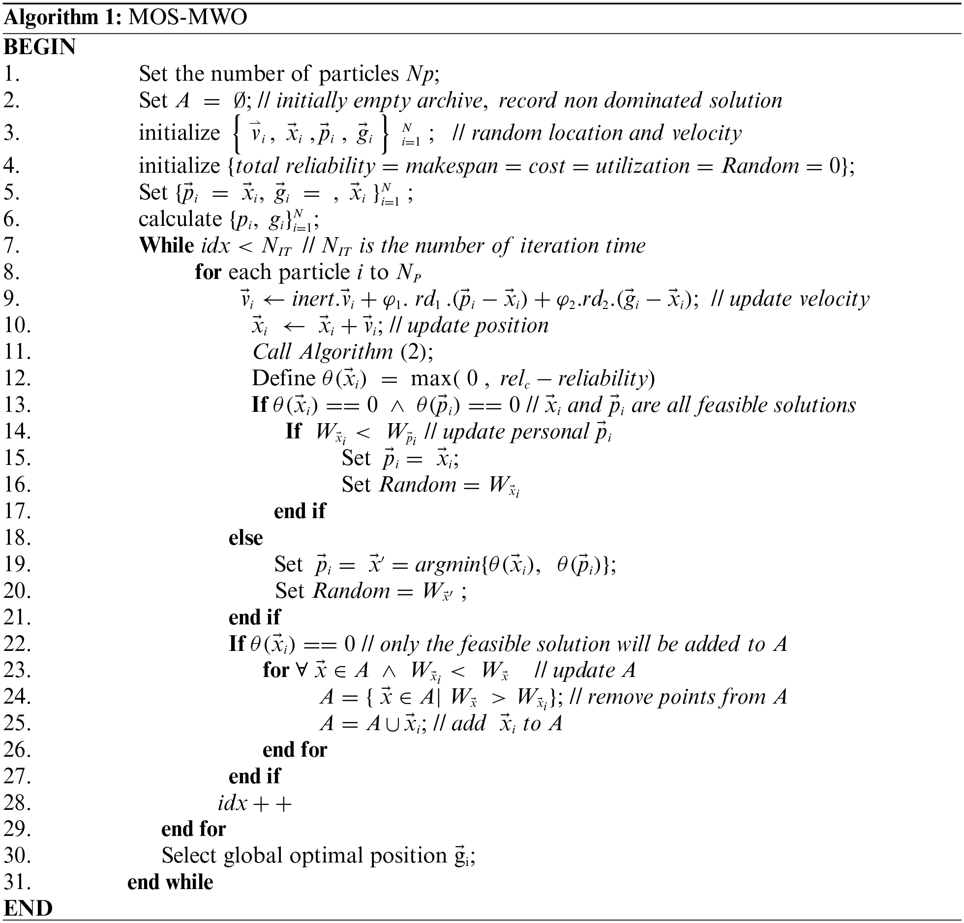
MOS-MWO scheduling algorithm involves estimating the fitness of each particle. Scheduling parameters and PSO parameters are initialized (lines 1–6). MOS-MWO calls Algorithm 2 to calculate the QoS parameters (line 11). There are two reliability constraints for selecting the viable solution [58]: 1) The optimal solution within the set of possible solutions (lines 13–17). In this case, a Random variable takes the weight of the optimal solution. 2) If not all solutions are feasible, the best solution and the Random value shall be chosen with the least reliability constraint (lines 18–21) [38]. So, only feasible solutions are stored (lines 22–27). The selected method is used to evaluate the optimal location (line 30) for multi-objective problems according to the weight of the alternative. The algorithm continues until the final condition is fulfilled (line 7).
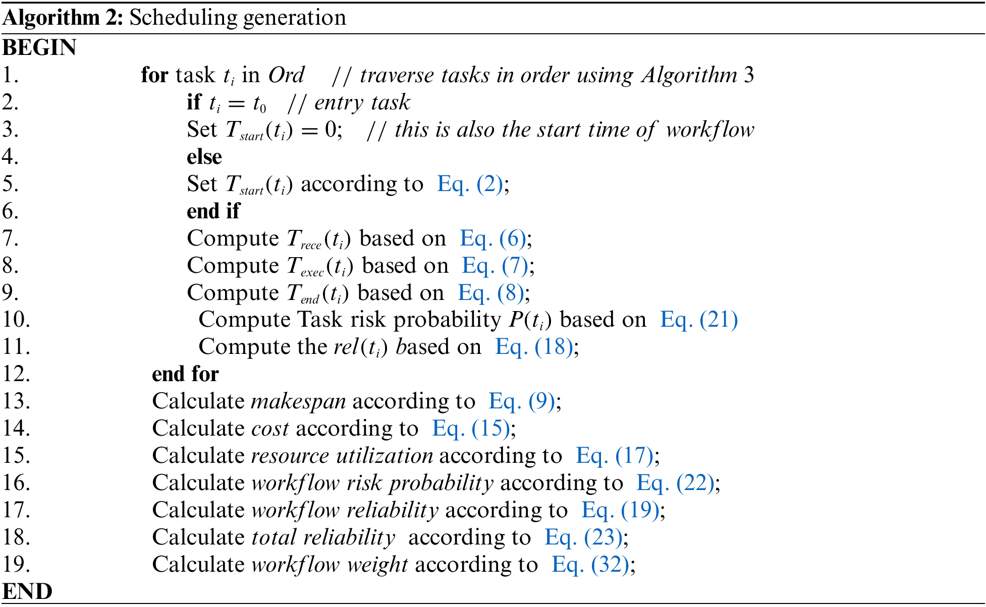
The output parameters are evaluated by scheduling generation (Algorithm 2) (lines 7–18) and tasks are traversed in order (line 1) using Algorithm 3 during the workflow scheduling process. The start time is calculated to find the makespan for each task (lines 2–6). Next, receiving data time Trece(ti), task execution time Texec(ti) and end time Tend(ti) are calculated (lines 7–9). The risk probability and reliability of the task (lines 10–11) then cost, reliability, resources utilization, risk probability and makespan of the workflow are determined (lines 13–18). The total reliability is calculated using Eq. (23) (line 18) and the minimum weight using Eq. (32). Finally, the weight of the workflow is calculated (line 19).

Algorithm 3 identifies task order according to the dependencies between tasks, that is, task t1must be executed before task t2 if it precedes task t2 in string Ord. Firstly, the scheduled tasks are initialized, i.e.,
6 Experimental Setup and Simulation Results
Fig. 3 shows the structure of the scientific workflow. Experiments were carried out using an i7 6 cores computer with a 16 GB RAM CPU. The proposed algorithm was implemented in Workflowsim 1.0 using four real-world scientific workflows; SIPHT, montage, LIGO and CyberShake. Random rd1 and rd2 values were generated by uniform distribution in the range [0, 1] with [1,32] computing units; respectively. The various cloud failure coefficients for Amazon EC2, Google Compute Engine and Microsoft Azure were identified as λ1 = 0.001, λ2 = 0.003 and λ3 = 0.002, respectively. The bandwidth was set to 0.1 G/s if the VMs are located within the same cloud while the bandwidth of the VMs was set to 0.05 G/s if they are located in different clouds. In the multi-objective problem, the reliability of the workflow should be equal or greater than the reliability constraint according to Eq. (26). Maximum reliability can be calculated by Eq. (19).

Figure 3: Structure of scientific workflows [45]
In MOS-MWO, φ1 = φ2 = 2.05, and the number of particles NP = 50. For the MOS-MWO algorithm, the number of compensation solutions NS = 15, the repeat time NIT = 1000 and repeat programming is 20 times. Besides the maximum workflow reliability, we also measured the minimum workflow reliability (relmin) to provide sufficient reliability. Users can set the reliability of workflow as follows:
where ρ
In our experiments, we set the reliability constraint coefficient ρ as 0.2.
This section discusses the results obtained from the experiments above with two and five conflicting objectives. The simulations were carried out under reliability constraint on four scientific workflow applications (Montage, LIGO, SIPHT and CyberShake) using MOS-MWO and the original MOS algorithms. The purpose of each algorithm is to optimize the QoS constraints. Feasible solutions were determined according to the minimum weight of the alternatives.
6.2.1 The Two-Objective Case Study
This scenario minimized two objectives, makespan and cost, to get the best trade-off during the scheduling process. The results are shown in Fig. 4. Makespan and cost are two non-beneficial metrics so they are normalized according to Eq. (30) and the minimum weight is calculated using Eq. (41) below.

Figure 4: Makespan-cost trade-off on real world scientific workflow in the case of two objectives
By applying our proposed algorithm in Fig. 4a, makespan and cost reduced by 26% and 21%, respectively compared to original-MOS. In Fig. 4b, it can be observed that MOS-MWO scheduling on LIGO yields better makespan and cost as it achieves 15% and 21% reduction, respectively. Fig. 4c shows that when MOS-MWO was applied on CyberShake, the makespan reduced by 12% while cost also reduced by 24% as compared to the original MOS algorithm. The result of the makespan-cost trade-off on SIPHT workflow (Fig. 4d) indicates that the makespan is reduced by 39% and the cost reduced by 30% using MOS-MWO. Overall, applying our proposed MOS-MWO algorithm minimized makespan and cost and performs better than original-MOS.
6.2.2 The Five-Objective Case Study
We consider a scenario consisting of five important objectives in real-life applications: makespan, cost, resource utilization, reliability and risk probability. Resource utilization and risk probability are vital to the resource provider while the other objectives are particularly of concern to the users. This section discusses the results obtained from the experiments with these five conflicting objectives. Fig. 5 shows the results of deploying MOS-MWO and original-MOS algorithms for the different scientific workflows to obtain their optimum solutions. Results from the Montage workflow in Fig. 5a show that the MOS-MWO algorithm yields the best set of makespan-cost trade-offs as compared with original-MOS algorithm. With MOS-MWO, makespan is reduced by 28% as compared to the original MOS and cost is also reduced by 4%. Similarly, Fig. 5b shows that MOS-MWO produced the best set of alternatives in terms of makespan-cost trade-off on LIGO. It reduced makespan and cost by 35% and 8%, respectively when compared to original-MOS.
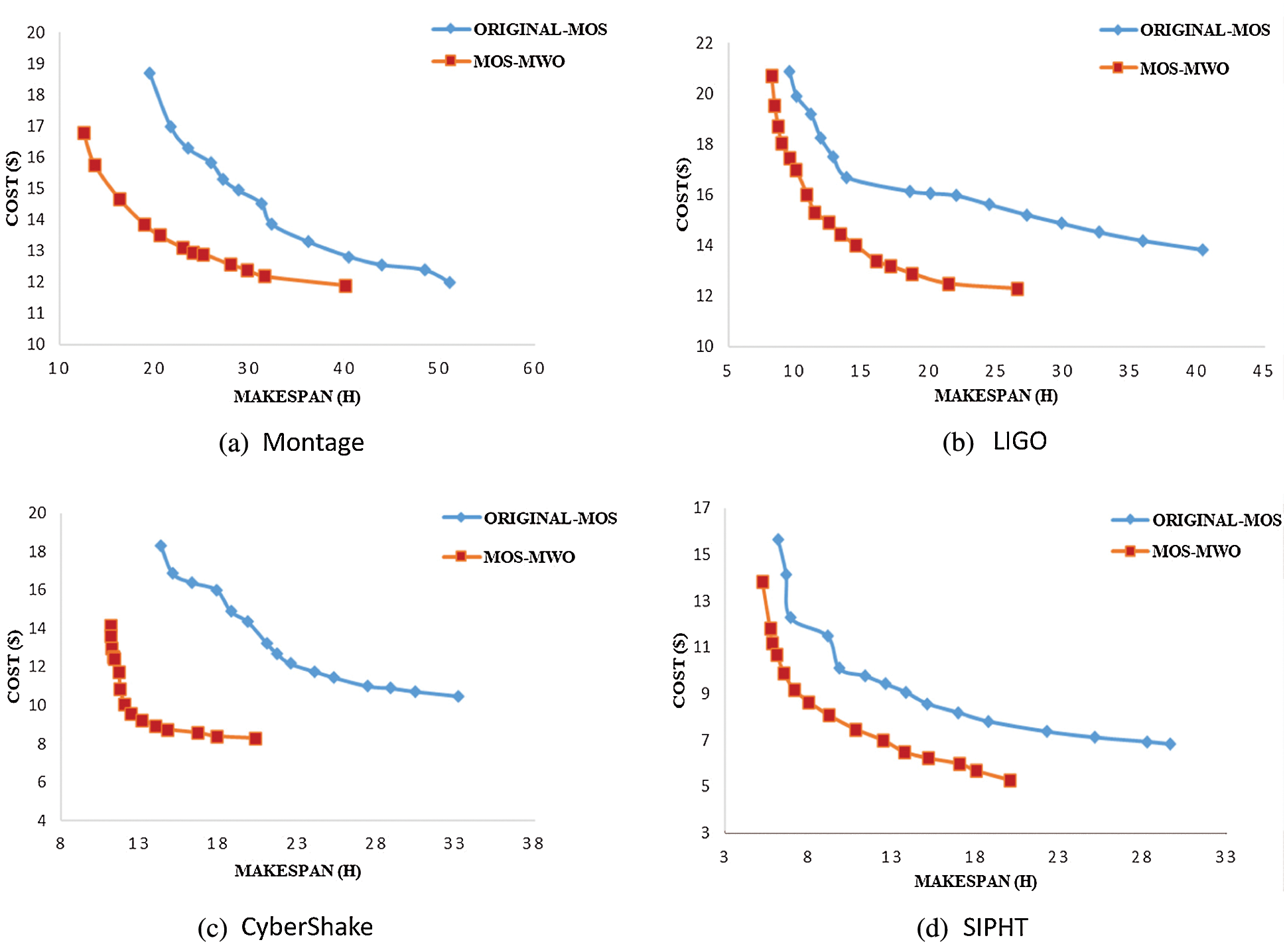
Figure 5: Makespan-cost trade-off on real world scientific workflow in case of five objectives
Looking at the two algorithms applied on CyberShake in Fig. 5c, results show that MOS-MWO produced solutions with the best makespan-cost trade-off. As compared to original-MOS, MOS-MWO reduced makespan and cost by 41% and 20%, respectively. This is also observed in the graphs for the SIPHT workflow (Fig. 5d). On applying MOS-MWO on SIPHT, we get a better makespan-cost trade-off and the makespan and cost reduced by 30% and 12%, respectively. Deductively, MOS-MWO outperforms original-MOS that applies the Pareto dominance method.
Fig. 6 shows the relationships between resource utilization and reliability. MOS-MWO and original-MOS algorithms are applied to various scientific workflows. Similar to Fig. 5, the results show that the MOS-MWO achieves the best performance (i.e., higher resource utilization and reliability) in comparison with the original MOS algorithm. This is an indication of the efficiency of our new decision-making method.
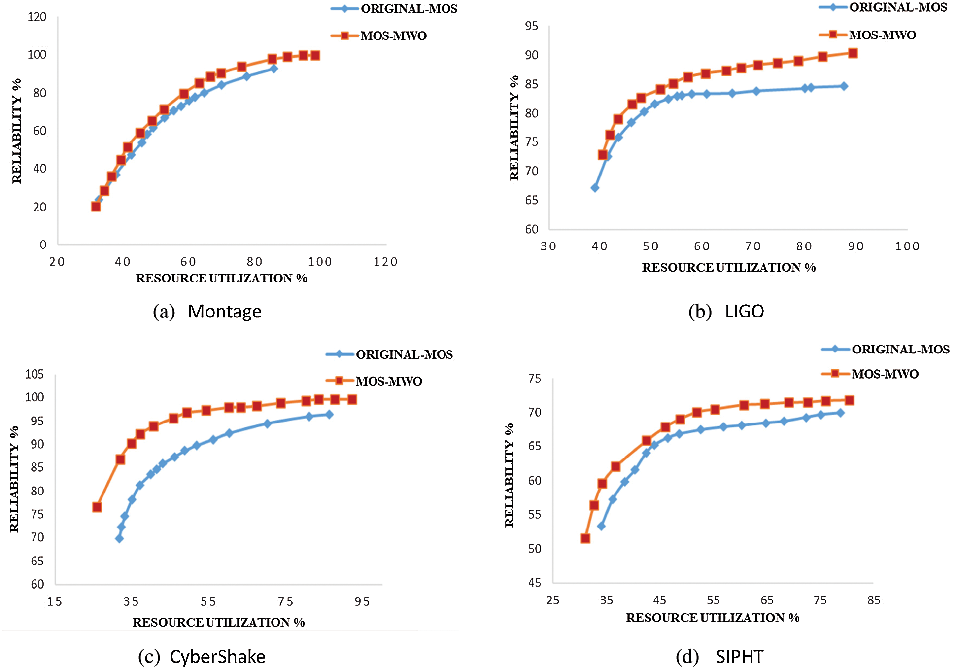
Figure 6: The relation between resource utilization and reliability
Fig. 6a shows that using MOS-MWO for scheduling Montage scientific workflow can produce better results in terms of reliability and resource utilization than original-MOS. The resource utilization and reliability increased by 13% and 15%, respectively when compared with original-MOS. Applying MOS-MWO on LIGO in Fig. 6b increased the resource utilization of MOS by 4%. The reliability also increased by 5% more than the original MOS. Fig. 6c shows that working with MOS-MWO on CyberShake gives best results in terms of resource utilization and reliability, so the resource utilization is 6% more than the original MOS and the reliability increased by about 4% more than original-MOS. As for SIPHT (Fig. 6d), we can see that MOS-MWO produced better results in terms of resource utilization with a 3% increase. Also, the reliability increased by 3% as compared to original-MOS.
Tab. 10 shows the results for the two multi-objective scheduling algorithms studied in this article. Both algorithms were executed in 1000 iterations to obtain the solutions with the highest reliability. With the conflicting attributes (makespan, cost, risk probability, reliability and resource utilization), the table shows that MOS-MWO yields the best results while working with all workflows. MOS-MWO performs better than the original MOS algorithm for all attributes. We noticed in Tab. 10 that in the case of SIPHT, original-MOS produces less cost as compared with MOS-MWO. This does not affect the overall performance because we are concerned about the general optimization of the scheduling process considering all the existing attributes. Nevertheless, MOS-MWO yields an optimal solution when compared with the original MOS algorithm.
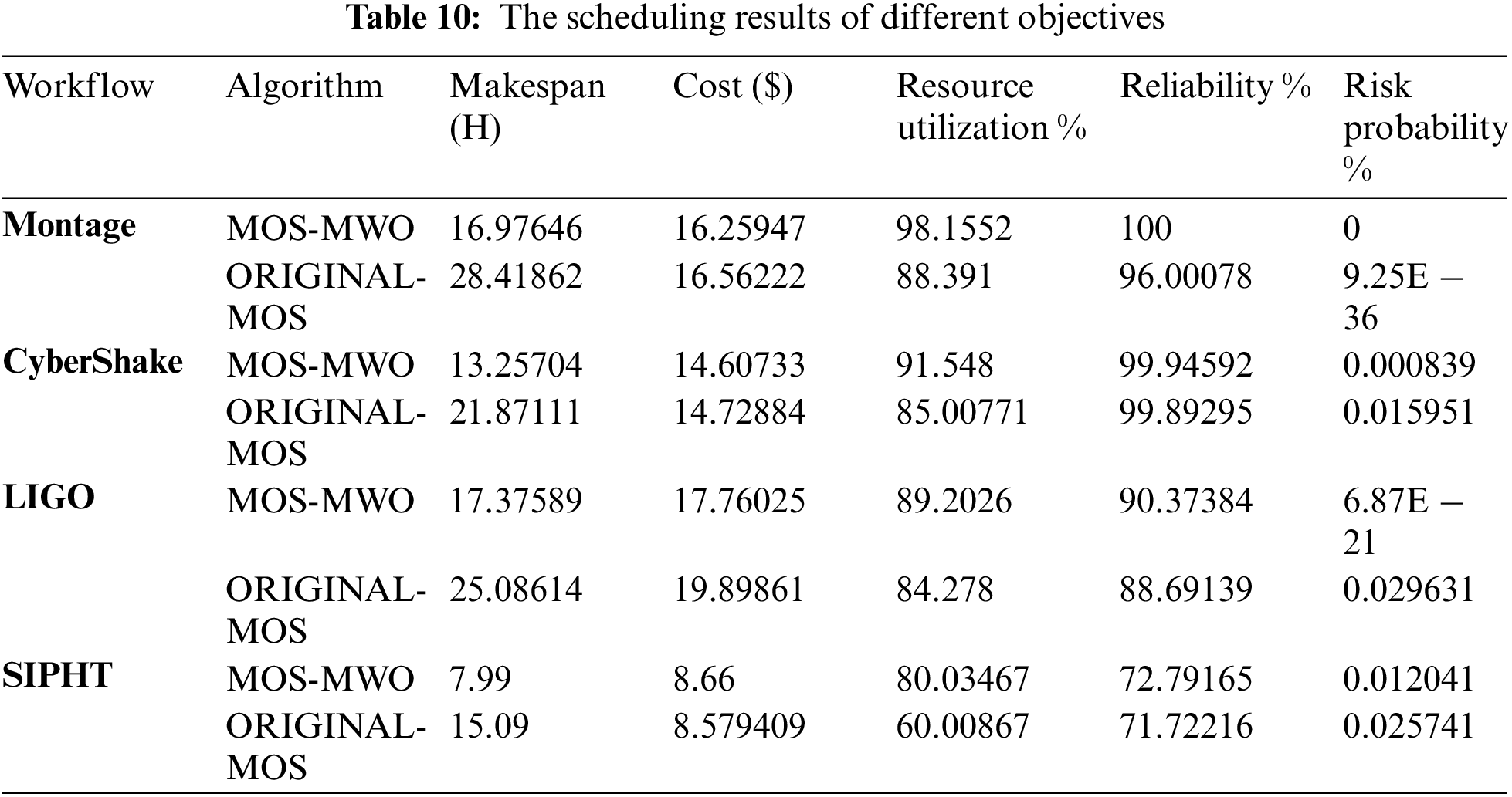
Fig. 7 shows the QoS satisfaction rate achieved by both MOS-MWO and original-MOS for all scientific workflows used in this study. As observed in Fig. 7a, MOS-MWO achieves the best QSR when dealing with Montage compared to original-MOS algorithm as it uses a number of iterations under the reliability constraint. MOS-MWO achieves a 2% improvement with respect to QSR while using 200 iterations and it achieved around 4% improvement of QSR when the number of iterations is 600. With 1000 iterations, MOS-MWO improved the satisfaction rate by 5% as compared with original-MOS. While increasing the number of iterations, we can get better QSR by using MOS-MWO.
Fig. 7b illustrates the results of scheduling LIGO scientific workflow by using both MOS-MWO and original-MOS under the reliability constraint. With 200 iterations, MOS-MWO yields about 3% QSR improvement as compared to MOS. By increasing the number of iterations to 1000, QSR increased by 4% when compared with original-MOS. Using MOS-MWO to schedule CyberShake in 200 iterations, the QSR improved by 3% more than original-MOS as shown in Fig. 7c. When the number of iterations increased to 1000, MOS-MWO improved QSR by 5% more than original-MOS.
Fig. 7d illustrates the results of scheduling SIPHT scientific workflow using both MOS-MWO and original-MOS algorithms under the reliability constraint. As compared to original-MOS, MOS-MWO achieves about 3% QSR improvement with 200 iterations. By increasing the number of iterations to 1000, the QSR increased to 5% in comparison with original-MOS.
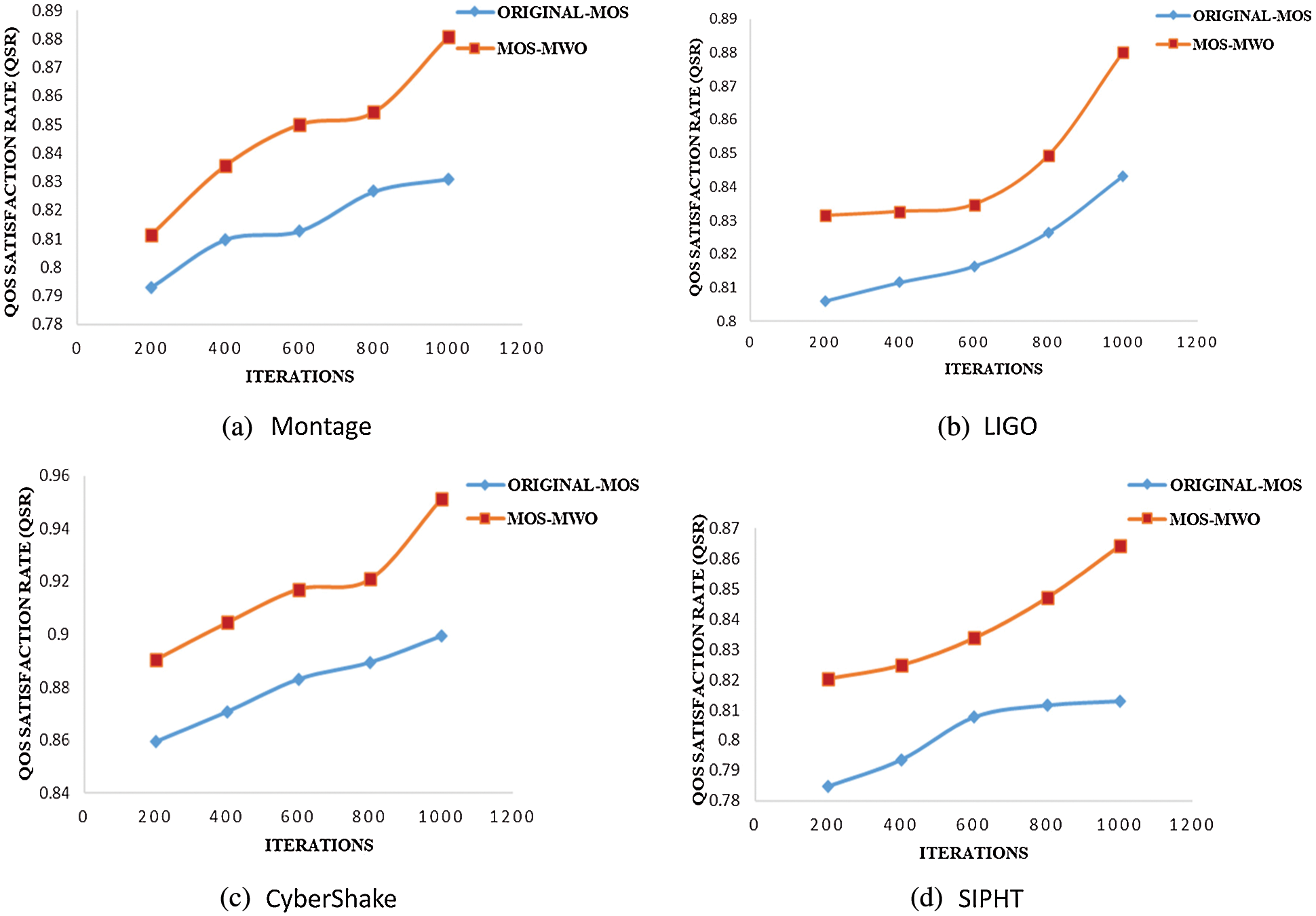
Figure 7: QoS satisfaction rate with five studied objectives
Examining just one of the aspects related to efficiency is unlikely to give a decisive test on multipurpose solutions. Thus, three metrics are used in this study: Q-metric, S-metric and FS-metric. These metrics are used to evaluate the quality of the Pareto fronts obtained by different algorithms [49]. Q-metric can be deployed [59,60] as shown in Eq. (42) to determine the particular degree of convergence of multi-objective algorithms A and B.
Ψ = Υ ∩ SA and Y is the set of SA ∪ SB. Two sets of Pareto optimum results for two multi-objective algorithms A and B are indicated by SA and SB. Algorithm A is better than Algorithm B only if Q(A, B) > Q(B, A) or Q(A, B) > 0.5. The Pareto front space size is determined by the FS metric as computed in Eq. (43) [61].
where fi(x0) and fi(x1) are two values of one objective function. A larger FS value means a greater diversity in the Pareto front. We adopt the S-metric as calculated in Eq. (44) in order to determine the level of uniformity of solutions [30].
where the number of Pareto solutions is NP and
A smaller S-metric implies that the algorithm has found a uniform solution, as opposed to FS-metric and Q-metric, where a greater value is preferred.
Figs. 5 and 6 show the trade-off between makespan and cost and the relation between reliability and resource utilization for MOS-MWO and original-MOS algorithms. Obviously, the MOS-MWO algorithm yields the optimal results for all objectives considered. The multi-objective performance metrics in Figs. 5 and 6 are illustrated in Tab. 11. If the Q-metrics of MOS-MWO is set to true, that implies that its performance is better than the original-MOS algorithm. Tab. 11 shows that the value of Q-metrics is true Q(MOS-MWO, MOS) for all scientific workflows. This shows that the solutions of MOS-MWO are always better than the original MOS, which means that MOS-MWO provides the best result in terms of multi-objective convergence.
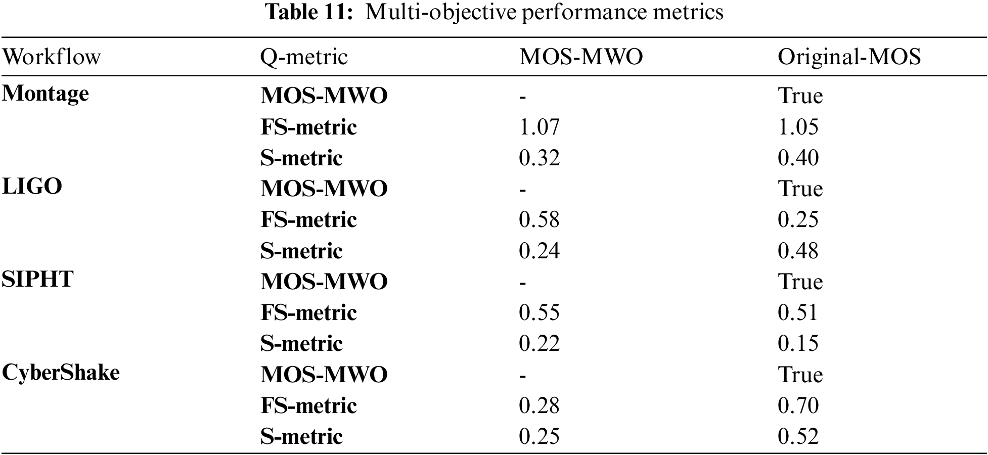
With regards to the Montage workflow, the FS-metric value for MOS-MWO is 1.07 which is greater than that of original-MOS algorithm. This means MOS-MWO achieves a higher diversity when compared to the original MOS algorithm. The S-metric for MOS-MWO is smaller than that of original-MOS algorithm by 0.02, which means MOS-MWO produces better uniformity in the Pareto front than the original MOS algorithm. As for the LIGO workflow, the FS-metric of MOS-MWO is 0.58 and that is higher than original-MOS algorithm thus, indicating that the MOS-MWO is better than original-MOS algorithm in terms of diversity. The value of the S-metric of MOS-MWO is lesser than that of the MOS algorithm by 0.24, which indicates the uniformity in the Pareto front of MOS-MWO is better than the original MOS algorithm.
In Tab. 11 we can see that applying MOS-MWO on SIPHT produced an FS-metric value of 0.55 which is better than the original MOS. In contrast, the S-metric of MOS-MWO is 0.22 which is higher than the original MOS algorithm. This implies that the uniformity produced by the original MOS is better than MOS-MWO algorithm. Looking at the results from the CyberShake, it can be observed that the FS-metric of MOS-MWO is 0.28 which is less than the original MOS algorithm that has 0.70 FS-metric value. This implies that original MOS produced a better diversity compared to the MOS-MWO algorithm. The S-metric value of MOS-MWO is 0.25 which is smaller than the original MOS. As such, MOS-MWO produces better uniformity when compared to original-MOS algorithm.
In this article, the MOS-MWO algorithm is presented and its efficiency in handling scheduling problems with multiple QoS constraints and objectives in a multi-cloud environment is demonstrated. The proposed MOS-MWO algorithm uses a novel decision-making method (MWO) to solve workflow scheduling problems by considering both users’ and service providers’ QoS requirements in multi-cloud environments. The proposed approach is modeled to handle QoS objective optimization with multiple constraints. MWO is used to evaluate and select the best solutions according to the weights of the specified alternatives. Such weights are also used to establish the inertia weight by using an adaptive strategy. High inertia weight means that the solution is not optimum thus, there is a need to increase exploration in the global search space to get good solutions. A low inertia weight means that the solution is near-optimal. Hence, we increase the exploitation in local search space to refine the solution and prevent big jumps in the search space. Extensive simulations were conducted on four scientific workflow applications to evaluate the performance of the proposed MOS-MWO algorithm. The simulation results obtained indicated that MOS-MWO outperformed the original MOS with respect to the QoS constraints. It also remarkably outperformed the original MOS in term of QoS satisfaction rate.
Acknowledgement: Throughout the study, the authors gratefully appreciate all those who contributed academically, technically, administratively and financially to this study.
Funding Statement: This work was supported by Putra Grant, University Putra Malaysia, under Grant 95960000 and in part by the Ministry of Education (MOE) Malaysia.
Conflicts of Interest: The authors declare that they have no conflicts of interest to report regarding the present study.
1. F. Ebadifard and S. Babamir “Dynamic task scheduling in cloud computing based on Naïve Bayesian classifier,” in Proc. of the Int. Conf. for Young Researchers in Informatics, Mathematics and Engineering Kaunas, Kaunas, Lithuania, vol. 1852, pp. 91–95, 2017. [Google Scholar]
2. B. Lin, W. Guo, G. Chen, N. Xiong and R. Li, “Cost-driven scheduling for deadline-constrained workflow on multi-clouds,” in 2015 IEEE Int. Parallel and Distributed Processing Symp. Workshop, Hyderabad, India, pp. 1191–1198, 2015. [Google Scholar]
3. N. Sooezi, S. Abrishami and M. Lotfian, “Scheduling data-driven workflows in multi-cloud environment,” in 2015 IEEE 7th Int. Conf. on Cloud Computing Technology and Science (CloudCom), Vancouver, BC, Canada, pp. 163–167, 2015. [Google Scholar]
4. L. Liu and M. Zhang, “Multi-objective optimization model with AHP decision-making for cloud service composition,” KSII Transactions on Internet and Information Systems (TIIS), vol. 9, no. 9, pp. 3293–3311, 2015. [Google Scholar]
5. F. Cappelletti, P. Penna, A. Prada and A. Gasparella, “Development of algorithms for building retrofit,” in Start-Up Creation. Smart Eco-Efficient Built Environment, Sawston, Cambridge, United Kingdom: Woodhead Publishing, pp. 349–373, 2016. [Google Scholar]
6. F. Ebadifard and S. Babamir, “A Multi-objective approach with WASPAS decision-making for workflow scheduling in cloud environment,” International Journal of Web Research, vol. 1, no. 1, pp. 1–10, 2018. [Google Scholar]
7. J. Li, S. Su, X. Cheng, Q. Huang and Z. Zhang, “Cost-conscious scheduling for large graph processing in the cloud,” in Proc. IEEE Int. Conf. on High Performance Computing and Communications, Banff, AB, Canada, pp. 808–813, 2011. [Google Scholar]
8. E. Jeannot, E. Saule and D. Trystram, “Optimizing performance and reliability on heterogeneous parallel systems: Approximation algorithms and heuristics,” Journal of Parallel and Distributed Computing, vol. 72, no. 2, pp. 268–280, 2012. [Google Scholar]
9. G. C. Sih and E. A. Lee, “A compile-time scheduling heuristic for interconnection-constrained heterogeneous processor architectures,” IEEE Transactions on Parallel and Distributed Systems, vol. 4, no. 2, pp. 175–187, 1993. [Google Scholar]
10. A. Doǧan and F. Özgüner, “Biobjective scheduling algorithms for execution time-reliability trade-off in heterogeneous computing systems,” The Computer Journal, vol. 48, no. 3, pp. 300–314, 2005. [Google Scholar]
11. S. Sagnika, M. Das and S. Bilgaiyan, “A Multi-objective cat swarm optimization algorithm for workflow scheduling in cloud computing environment,” Intelligent Computing, Communication and Devices, vol. 2, pp. 73–84, 2015. [Google Scholar]
12. O. Udomkasemsub, L. Xiaorong and T. Achalakul, “A Multiple-objective workflow scheduling framework for cloud data analytics,” in Ninth Int. Conf. on Computer Science and Software Engineering (JCSSE), Bangkok, Thailand, IEEE, pp. 391–398, 2012. [Google Scholar]
13. Z. Wu, Z. Ni, L. Gu and X. Liu, “A revised d iscrete particle swarm optimization for cloud workflow scheduling,” in 2010 Int. Conf. on Computational Intelligence and Security, Nanning, Guangxi Zhuang Autonomous Region China, pp. 184–188, 2010. [Google Scholar]
14. A. Khalili and S. M. Babamir, “Optimal scheduling workflows in cloud computing environment using Pareto-based grey wolf optimizer,” Concurrency and Computation: Practice and Experience, vol. 29, no. 11, pp. 1–11, 2017. [Google Scholar]
15. S. Yassa, R. Chelouah, H. Kadima and B. Granado, “Multi-objective approach for energy-aware workflow scheduling in cloud computing environments,” The Scientific World Journal, vol. 2013, Article ID. 350934, pp. 1–13, 2013. [Google Scholar]
16. F. Ebadifard and S. M. Babamir, “Scheduling scientific workflows on virtual machines using a Pareto and hypervolume based black hole optimization algorithm,” The Journal of Supercomputing, vol. 76, pp. 1–54, 2020. [Google Scholar]
17. P. Kaur and S. Mehta, “Resource provisioning and work flow scheduling in clouds using augmented shuffled frog leaping algorithm,” Journal of Parallel and Distributed Computing, vol. 101, pp. 41–50, 2017. [Google Scholar]
18. M. Zhang, H. Li, L. Liu and R. Buyya, “An adaptive multi-objective evolutionary algorithm for constrained workflow scheduling in clouds,” Distributed and Parallel Databases, vol. 36, no. 2, pp. 339–368, 2018. [Google Scholar]
19. V. Singh, I. Gupta and P. K. Jana, “An energy efficient algorithm for workflow scheduling in IAAS cloud,” Journal of Grid Computing, vol. 18, no. 3, pp. 357–376, 2019. [Google Scholar]
20. A. Verma and S. Kaushal, “A hybrid multi-objective particle swarm optimization for scientific workflow scheduling,” Parallel Computing, vol. 62, pp. 1–19, 2017. [Google Scholar]
21. N. V. Dharwadkar, S. R. Poojara and P. M. Kadam, “Fault tolerant and optimal task clustering for scientific workflow in cloud,” International Journal of Cloud Applications and Computing, vol. 8, no. 3, pp. 1–19, 2018. [Google Scholar]
22. J. J. Durillo, H. M. Fard and R. Prodan, “MOHEFT: A multi-objective list-based method for workflow scheduling,” in 4th IEEE Int. Conf. on Cloud Computing Technology and Science Proc., Taipei, Taiwan, pp. 185–192, 2012. [Google Scholar]
23. J. J. Durillo and R. Prodan, “Multi-objective workflow scheduling in Amazon EC2,” Cluster Computing, vol. 17, no. 2, pp. 169–189, 2014. [Google Scholar]
24. J. J. Durillo, R. Prodan and J. G. Barbosa, “Pareto tradeoff scheduling of workflows on federated commercial clouds,” Simulation Modelling Practice and Theory, vol. 58, no. 2, pp. 95–111, 2015. [Google Scholar]
25. J. Yu, R. Buyya and K. Ramamohanarao, “Workflow scheduling algorithms for grid computing,” Metaheuristics for Scheduling in Distributed Computing Environments, vol. 146, pp. 173–214, 2008. [Google Scholar]
26. M. Kalra and S. Singh, “Multi-criteria workflow scheduling on clouds under deadline and budget constraints,” Concurrency and Computation: Practice and Experience, vol. 31, no. 17, pp. 1–16, 2019. [Google Scholar]
27. I. Casas, J. Taheri, R. Ranjan and A. Y. Zomaya, “PSO-DS: A scheduling engine for scientific workflow managers,” The Journal of Supercomputing, vol. 73, no. 9, pp. 3924–3947, 2017. [Google Scholar]
28. Z. Zhu, G. Zhang, M. Li and X. Liu, “Evolutionary multi-objective workflow scheduling in cloud,” IEEE Transactions on Parallel and Distributed Systems, vol. 27, no. 5, pp. 1344–1357, 2016. [Google Scholar]
29. X. Zhou, G. Zhang, J. Sun, J. Zhou, T. Wei et al., “Minimizing cost and makespan for workflow scheduling in cloud using fuzzy dominance sort based HEFT,” Future Generation Computer Systems, vol. 93, pp. 278–289, 2019. [Google Scholar]
30. M. Farid, R. Latip, M. Hussin and N. A. W. Abdul Hamid, “Scheduling scientific workflow using multi-objective algorithm with fuzzy resource utilization in multi-cloud environment,” IEEE Access, vol. 8, pp. 24309–24322, 2020. [Google Scholar]
31. M. A. Rodriguez and R. Buyya, “Deadline based resource provisioning and scheduling algorithm for scientific workflows on clouds,” IEEE Transactions on Cloud Computing, vol. 2, no. 2, pp. 222–235, 2014. [Google Scholar]
32. Z. Li, J. Ge, H. H. Hu, W. Song, H. H. Hu et al., “Cost and energy aware scheduling algorithm for scientific workflows with deadline constraint in clouds,” IEEE Transactions on Services Computing, vol. 11, no. 4, pp. 713–726, 2015. [Google Scholar]
33. C. Zhang, R. Green and M. Alam, “Reliability and utilization evaluation of a cloud computing system allowing partial failures,” in IEEE 7th Int. Conf. on Cloud Computing, Anchorage, AK, USA, pp. 936–937, 2014. [Google Scholar]
34. S. Kianpisheh, N. M. Charkari and M. Kargahi, “Reliability-driven scheduling of time/cost-constrained grid workflows,” Future Generation Computer Systems, vol. 55, pp. 1–16, 2016. [Google Scholar]
35. D. Poola, K. Ramamohanarao and R. Buyya, “Enhancing reliability of workflow execution using task replication and spot instances,” ACM Transactions on Autonomous and Adaptive Systems (TAAS), vol. 10, no. 4, pp. 1–21, 2016. [Google Scholar]
36. Z. Li, J. Ge, H. Yang, L. Huang, H. Hu et al., “A security and cost aware scheduling algorithm for heterogeneous tasks of scientific workflow in clouds,” Future Generation Computer Systems, vol. 65, pp. 140–152, 2016. [Google Scholar]
37. L. Zeng, B. Veeravalli and X. Li, “SABA: A security-aware and budget-aware workflow scheduling strategy in clouds,” Journal of Parallel and Distributed Computing, vol. 75, pp. 141–151, 2015. [Google Scholar]
38. H. M. Fard, R. Prodan and T. Fahringer, “Multi-objective list scheduling of workflow applications in distributed computing infrastructures,” Journal of Parallel and Distributed Computing, vol. 74, no. 3, pp. 2152–2165, 2014. [Google Scholar]
39. L. Zhang, K. K. Li, C. Li and K. K. Li, “Bi-objective workflow scheduling of the energy consumption and reliability in heterogeneous computing systems,” Information Sciences, vol. 379, pp. 241–256, 2017. [Google Scholar]
40. X. Tang, K. Li, Z. Zeng and B. Veeravalli, “A novel security-driven scheduling algorithm for precedence-constrained tasks in heterogeneous distributed systems,” IEEE Transactions on Computers, vol. 60, no. 7, pp. 1017–1029, 2011. [Google Scholar]
41. T. Xie and X. Qin, “Performance evaluation of a new scheduling algorithm for distributed systems with security heterogeneity,” Journal of Parallel and Distributed Computing, vol. 67, no. 10, pp. 1067–1081, 2007. [Google Scholar]
42. T. Xie and X. Qin, “Scheduling security-critical real-time applications on clusters,” IEEE Transactions on Computers, vol. 55, no. 7, pp. 864–879, 2006. [Google Scholar]
43. Y. Wang, Y. Guo, Z. Guo, W. Liu and C. Yang, “Securing the intermediate data of scientific workflows in clouds with ACISO,” IEEE Access, vol. 7, pp. 126603–126617, 2019. [Google Scholar]
44. P. Wang, Y. Lei, P. R. Agbedanu and Z. Zhang, “Makespan-driven workflow scheduling in clouds using immune-based PSO algorithm,” IEEE Access, vol. 8, pp. 29281–29290, 2020. [Google Scholar]
45. H. Hu, Z. Li, H. Hu, J. Chen, J. Ge et al., “Multi-objective scheduling for scientific workflow in multicloud environment,” Journal of Network and Computer Applications, vol. 114, no. 11, pp. 108–122, 2018. [Google Scholar]
46. D. Araújo, C. Bastos-Filho, E. Barboza, D. Chaves and J. Martins-Filho, “A performance comparison of multi-objective optimization evolutionary algorithms for all-optical networks design,” IEEE Symposium on Computational Intelligence in Multicriteria Decision-Making (MDCM), Paris, France, vol. 2011 MDCM, pp. 89–96, 2011. [Google Scholar]
47. R. Eberhart and J. Kennedy, “A new optimizer using particle swarm theory,” in MHS'95. Proc. of the Sixth Int. Symp. on Micro Machine and Human Science, Nagoya, Japan, vol. 0-7803–267, pp. 39–43, 1995. [Google Scholar]
48. J. E. Alvarez-Benitez, R. M. Everson and J. E. Fieldsend, “A MOPSO algorithm based exclusively on pareto dominance concepts,” in Int. Conf. on Evolutionary Multi-Criterion Optimization, Guanajuato, Mexico, pp. 459–473, 2005. [Google Scholar]
49. J. Wei and M. Zhang, “A memetic particle swarm optimization for constrained multi-objective optimization problems,” IEEE Congress of Evolutionary Computation (CEC), vol. CEC 2011, pp. 1636–1643, 2011. [Google Scholar]
50. W. F. Leong and G. G. Yen, “PSO-Based multiobjective optimization with dynamic population size and adaptive local archives,” IEEE Transactions on Systems, Man, and Cybernetics, Part B (Cybernetics), vol. 38, no. 5, pp. 1270–1293, 2008. [Google Scholar]
51. H. P. Dai, D. D. Chen and Z. S. Zheng, “Effects of random values for particle swarm optimization algorithm,” Algorithms, vol. 11, no. 2, pp. 1–23, 2018. [Google Scholar]
52. Y. del Valle, G. K. Venayagamoorthy, S. Mohagheghi, J. -C. Hernandez and R. G. Harley, “Particle swarm optimization: Basic concepts, variants and applications in power systems,” IEEE Transactions on Evolutionary Computation, vol. 12, no. 2, pp. 171–192, 2008. [Google Scholar]
53. R. L. Oliver, “Effect of expectation and disconfirmation on postexposure product evaluations: An alternative interpretation,” Journal of Applied Psychology, vol. 62, no. 4, pp. 480–486, 1976. [Google Scholar]
54. N. Yadav, M. S. Goraya and D. Singh, “Satisfaction aware QoS-based bidirectional service mapping in cloud environment,” Cluster Computing, vol. 23, no. 4, pp. 2991–3011, 2020. [Google Scholar]
55. J. Kennedy and R. Eberhart, “Particle swarm optimisation,” in Proc. of ICNN'95-Int. Conf. on Neural Networks, Perth, WA, Australia, vol. 4, pp. 1942–1948, 1995. [Google Scholar]
56. Y. Shi and R. Eberhart, “A modified particle swarm optimizer,” in IEEE Int. Conf. on Evolutionary Computation Proc. IEEE World Congress on Computational Intelligence (Cat. No. 98TH8360), Anchorage, AK, USA, pp. 69–73, 1998. [Google Scholar]
57. R. C. Eberhart and Y. Shi, “Tracking and optimizing dynamic systems with particle swarms,” in Proc. of the 2001 Congress on Evolutionary Computation (IEEE Cat. No. 01TH8546), Seoul, Korea (Southvol. 1, pp. 94–100, 2001. [Google Scholar]
58. K. Deb, “An efficient constraint handling method for genetic algorithms,” Computer Methods in Applied Mechanics and Engineering, vol. 186, no. 2–4, pp. 311–338, 2000. [Google Scholar]
59. W. Jing, Z. Yongsheng, Y. Haoxiong and Z. Hao, “A Trade-off pareto solution algorithm for multi-objective optimization,” in Fifth Int. Joint Conf. on Computational Sciences and Optimization. IEEE, Harbin, China, pp. 123–126, 2012. [Google Scholar]
60. J. Hartmanis and J. Van Leeuwen, “Advances in natural computation,” in Second Int. Conf., ICNC 2006, Xi'an, China, Proc., Part II. vol. 4222, 2006. [Google Scholar]
61. R. Garg and A. K. Singh, “Multi-objective workflow grid scheduling using ε-fuzzy dominance sort based discrete particle swarm optimization,” The Journal of Supercomputing, vol. 68, no. 2, pp. 709–732, 2014. [Google Scholar]
 | This work is licensed under a Creative Commons Attribution 4.0 International License, which permits unrestricted use, distribution, and reproduction in any medium, provided the original work is properly cited. |