DOI:10.32604/cmc.2022.022457
| Computers, Materials & Continua DOI:10.32604/cmc.2022.022457 | |
| Article |
Efficient Classification of Remote Sensing Images Using Two Convolution Channels and SVM
1ENSA, Abdelmalek Essaadi University, Tetouan 93002, Morocco
2FS, Abdelmalek Essaadi University, Tetouan 93002, Morocco
3Department of Electrical Engineering, Faculty of Engineering, Menoufia University, Shebin El-Kom 32511, Egypt
4Department of Computer Engineering, College of Computers and Information Technology, Taif University, P.O. Box 11099, Taif 21944, Saudi Arabia
5ENSIAS, Mohammed V University in Rabat 10000, Morocco
6Department of Information Technology, College of Computers and Information Technology, Taif University, P.O. Box 11099, Taif 21944, Saudi Arabia
*Corresponding Author: Mohammed Baz. Email: mo.baz@tu.edu.sa
Received: 08 August 2021; Accepted: 01 December 2021
Abstract: Remote sensing image processing engaged researchers’ attentiveness in recent years, especially classification. The main problem in classification is the ratio of the correct predictions after training. Feature extraction is the foremost important step to build high-performance image classifiers. The convolution neural networks can extract images’ features that significantly improve the image classifiers’ accuracy. This paper proposes two efficient approaches for remote sensing images classification that utilizes the concatenation of two convolution channels’ outputs as a features extraction using two classic convolution models; these convolution models are the ResNet 50 and the DenseNet 169. These elicited features have been used by the fully connected neural network classifier and support vector machine classifier as input features. The results of the proposed methods are compared with other antecedent approaches in the same experimental environments. Evaluation is based on learning curves plotted during the training of the proposed classifier that is based on a fully connected neural network and measuring the overall accuracy for the both proposed classifiers. The proposed classifiers are used with their trained weights to predict a big remote sensing scene's classes for a developed test. Experimental results ensure that, compared with the other traditional classifiers, the proposed classifiers are further accurate.
Keywords: Remote sensing images; deep learning; ResNet; DenseNet; SVM
With the quick evolution of communications, remote sensing images were known after the advent of cameras and satellites. For transacting with the nature of these images, it is required to process this type of images. Classification is one of the essential processes for these images. The classification process can be fulfilled using machine and deep learning technologies. One of the artificial intelligence sections is machine learning which relies on coaching computers using real data, which results in computers making strong predictions for the same form of data as an expert human [1]. One of machine learning's important portions is deep learning. The artificial neural networks (ANNs) are the main ground for deep learning, where remote sensing images classifiers are one of the deep learning applications [2]. With the availability of cameras with high spatial and spectral resolutions, which can be located on later satellite versions, remote sensing scenes with very high resolution (VHR) have emerged. The VHR images in remote sensing have redundancy pixels as a fair outcome, which can cause an over-fitting problem during coaching using deep learning or machine learning. So, the ANNs must be improved, and useful features from remote sensing images must be extracted as an initial step before coaching [3]. The convolution neural networks (CNNs), which have thrilling rapid progress in computer vision, are inherited from the ANNs but without fully linked layers as the ANNs layers [4–6]. Classification is an important issue from computer vision issues [6]. The classic networks have seemed as CNNs deep networks with particular construction, giving rise to rising precisions in the classification issues. This is due to the need to process materials containing a huge amount of data as contained in the high-resolution images. Two classic networks have been used as feature extraction in the proposed methods presented by this paper; the DenseNet 169 and the ResNet 50 models. Many researchers attempted to reach good predictions for the remote sensing images classifiers. Liu et al. [7] compared the deep learning classifiers and the support vector machine (SVM) classifier for remote sensing images. Guo et al. [8] used a sequential classifier and SVM for proposing an effective algorithm that classifies remote sensing images. Sukawattanavijit et al. [9] used SVM classifier and genetic algorithm to suggest a remote sensing images classification approach. Liu et al. [10] utilized SVM classifier and Gustafson–Kessel fuzzy clustering algorithm to propose a novel learning model. This model has been trained with a few labeled remote sensing images and some unlabeled remote sensing images. Petropoulos et al. [11] utilized two classifiers, the pixel-based SVM classifier and object-based classifier, to evaluate the Hyperion sensor performance. Wang et al. [12] elicited convolution features from the VHR images in remote sensing by utilizing the ResNet 50 model and then concatenated these convolution features with low-level features to produce input features for the SVM classifier and then they built their proposed classifier. Jiang et al. [13] elicited 3-D features from the hyperspectral remote sensing images by utilizing the ResNet 50 model to build their proposal. Natesan et al. [14] distinguished the forest tree species by utilizing the ResNet 50 model to build their proposed classifier. The used dataset in their research is formed from RGB images with high resolution. The authors used an unmanned aerial vehicle (UAV) fitted with a simple-pitch camera for picking these images. Yang et al. [15] used super vector coding and ResNet 50 to propose airplanes’ detection approach. Xu et al. [16] suggested an approach for classifying remote sensing images by utilizing the ResNet 50 model with a combination of edge and texture maps. Tao et al. [17] improved the accuracy of a remote sensing images classifier that utilized the DenseNet 169 model. Yang et al. [18] utilized the DenseNet 169 to construct two CNNs paths for debriefed convolution features from remote sensing images. Zhang et al. [19] suggested a remote sensing image classifier by utilizing the DenseNet 169 model. They utilized dense connections to build a small aggregate of convolution kernels to realize many reusable feature maps. AlAfandy et al. [20] compared four remote sensing images’ classifiers that utilized four classic networks; the VGG 16, the ResNet 50, the NASNet Mobile, and the DenseNet 169 models. Transfer learning was done for these networks, and then fully connected (FC) layers were created and retrained. AlAfandy et al. [21] proposed three remote sensing images’ classifiers based on classic networks and SVM. They utilized three classic models as features extraction; the VGG 16, the DenseNet 169, and the ResNet 50 models. Transfer learning was done for these networks to produce the extracted features; these features have been invested as input features for SVM models training.
The addressed issue in this article is the complexity of achieving elevated correct predictions precision in remote sensing images classifiers. Several researchers have suggested solutions to this issue, but they rely only on machine learning or deep learning. Not many have suggested crossbred approaches from a mixture of deep learning and machine learning, such as [9,12,21].
This paper aims to propose efficient remote sensing images’ classification methods with high correct predictions’ accuracies. These methods are based on using two convolution channels for debriefing the desired features from the remote sensing images by concatenating the outputs of these convolution channels. These two convolution channels are two deep classic networks with ImageNet pre-trained weights after transfer learning; these models are the ResNet 50 and DenseNet 169 models. In these two networks, the transfer learning is done to the output layer's previous layer, which is the last hidden layer. These debriefed features have been deemed as input features for two classifiers. One of these classification methods is a FC layer (an output layer), which has a softmax activation function, convenient with the used dataset classes. The other classification method is the SVM model. These classifiers have been trained using remote sensing images datasets. The SIRI-WHU dataset and the UC Merced land use dataset are utilized for training the proposed models in this paper. There are two steps to assess the efficiency of these proposals; the first step is comparing the experimental results of these proposed methods with the antecedent results in [20,21]. This comparative is done by measuring the overall accuracy (OA) for each classifier. The other step is using the proposed classifiers with their trained weights to predict the classes of a big remote sensing scene. In the FC model, one additional test is utilized which is the learning curves plots to determine the hyper-parameters forces.
The remainder of this article is structured as follows. Methods are described in Section 2. In Section 3, the experimental results and setup are discussed. The conclusion is given in Section 4 and followed by the declarations and the most relevant references.
The proposed classifiers, with their structures, are explained in this section. The SVM classifiers and the invested classic networks in these proposals will be summarized, followed by measuring the learning model performance as a literature review.
The main backbone in the remote sensing images classification is feature extraction. So, the idea of the proposed classification methods in this paper is that the concatenation of two convolution channels outputs is employed to bring out images features. These features are utilized to feed two classifiers as inputs for coaching these classifiers.
The first channel uses the ResNet 50 model. The other channel uses the DenseNet 169 model. The first classifier is the creation of a FC layer with softmax activation function, and the other classifier is the SVM classifier. For the two convolution channels, the transfer learning is done to the output layer's previous layer, which is the last hidden layer; the first channel output, according to the ResNet 50 structure, consists of 2048 neurons where the second channel output, according to the DenseNet 169 structure, consists of 1664 neurons. Fig. 1 shows the two convolution channels that used to extract features.
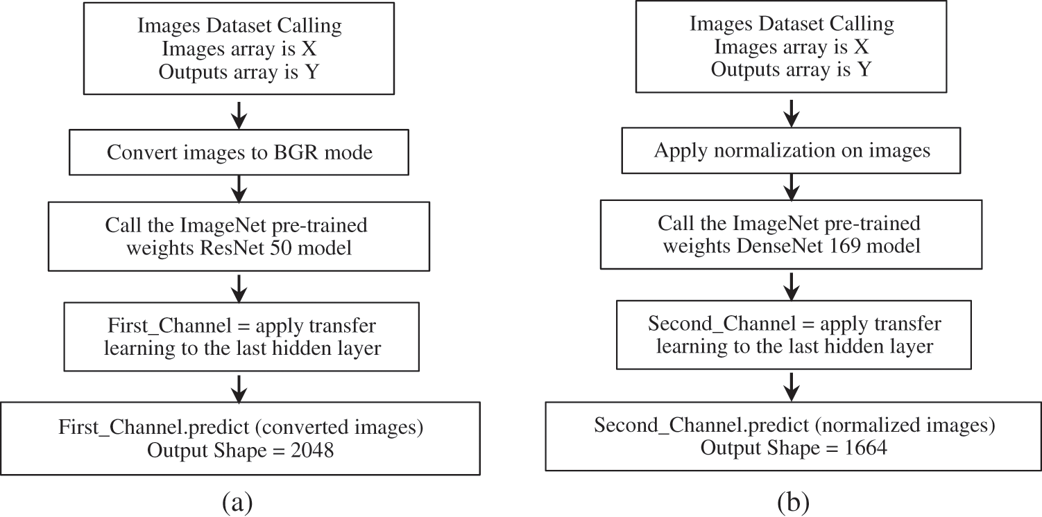
Figure 1: The two convolution channels that used to extract features. (a) The first convolution channel (based on ResNet 50) (b) The second convolution channel (based on DenseNet 169)
The desired extracted features are produced by concatenating the outputs of these two convolution channels that will be 3712 neurons. The ImageNet pre-trained weights are utilized because a large amount of data has been needed to train new models of CNNs. Fig. 2 shows the proposed methods.
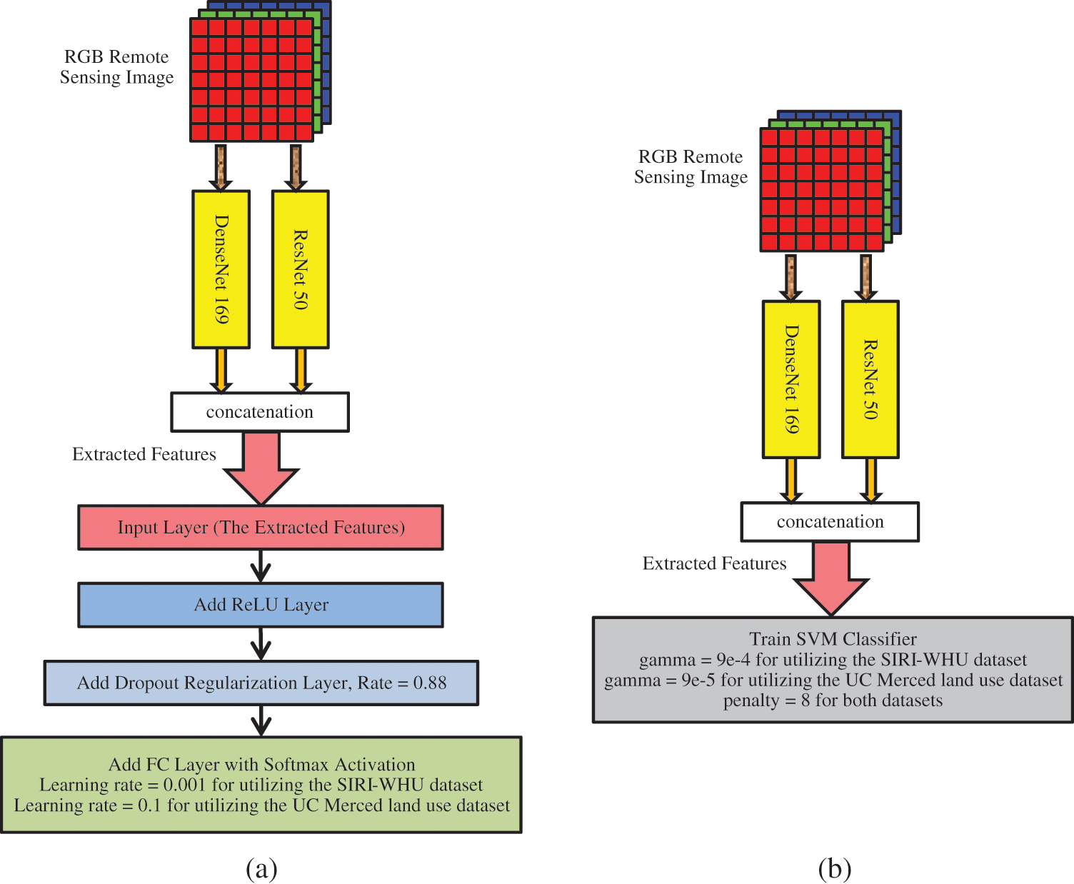
Figure 2: The proposed methods. (a) The proposed FC classifier (b) The proposed SVM classifier
2.2 The Support Vector Machine (SVM)
One of the broad hired machine learning algorithms is the SVM. The SVM algorithm acts as a regression or classifier. It gives a good separation of classes when used as a supervised classification model. The basic idea of the SVM classifier is to generate optimal hyper-planes from the training data by utilizing small statistical theory. These hyper-planes have been created by decision planes that define decision boundaries [22,23]. The SVM structure is challenging to understand. By building margins between classes, the hyper-plans distinguish the various classes. The main track to achieve the optimal SVM classifier is to maximize these margins on both aspects of hyper-planes, especially the nearest classes. For the SVM classifier, the cost function can be represented as Eq. (1) and the hypothesis function can be represented as Eq. (2) [22,23]:
Fig. 3 shows the SVM classifier [23].
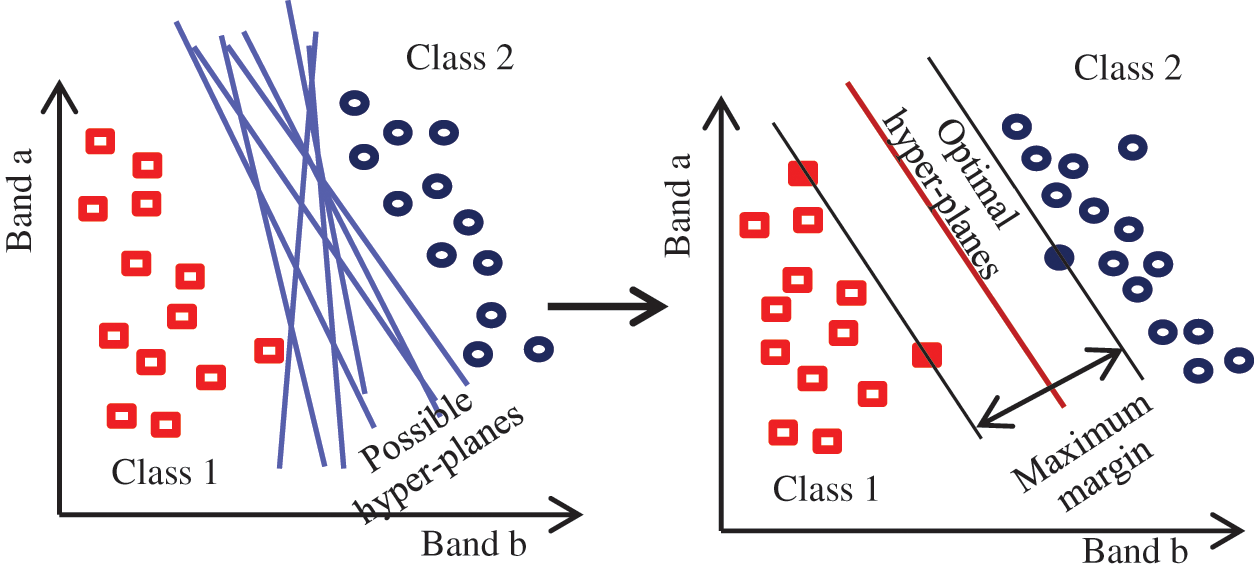
Figure 3: The SVM classifier [23]
In 2016, He et al. [24] proposed the ResNet 50 models. The authors exhibit a deep residual learning framework. The authors aim, from their proposal, to facilitate the training of the networks, which are deeper than previous. This proposed learning framework assists in addressing the degradation problem. Rather than hoping every small number of stacked layers appropriate the desirable underlying mapping directly, authors allowed these layers specifically to appropriate a residual mapping.
The idea of ResNet 50 is to create bypass connections that are connecting the deep layers with bypassing non-linear transformation layers. The block output is the addition of these connections’ outputs and network stack layers’ outputs as Eq. (3) [24]:
where

Figure 4: The one building block ResNet [24]
In 2017, the DenseNet 169 models were proposed by Huang et al. [25]. The beginning was a study prepared by authors about the effect of having any links between CNNs layers. Then, the authors attempted to create deep CNNs with shorter links among substantial layers near the input and those near the output. The result showed that deep CNNs models that contain shorter links between layers are effective to train and more precise. The DenseNets have full layers connections. In DenseNets, any layer has direct connections to other subsequent layers.
So the
where

Figure 5: The 5 layers dense block structure [25]
2.5 The Performance Assessment
The efficiency of the learning models is calculated by several matrices. The OA is the widely used and the main assessment [26,27]. It measures the percentage ratio between test data correct predictions and all dataset's test data objects. The OA can be represented as Eq. (5) [26,27].
3 The Experimental Setup and Results
This section illustrates the proposed methods’ experiments setup and results and compares these proposed methods with previous methods’ results in [20] and [21]. This comparison is established according to the OA measurements for each model. For the FC layer proposal, to measure the competence of this method's used hyper-parameters, the learning curves have been plotted. The used datasets for training the proposed classification methods are the SIRI-WHU dataset and the UC Merced land use dataset. A developed test for the proposed classifier is done by predicting the classes of a big remote sensing scene using the proposed models with their trained weights. This scene was taken from the library of the United States Geological Survey (USGS) agency. All of the used datasets’ images are Geo-tiff RGB images where the Geo-tiff RGB images, in remote sensing, are similar to RGB images [28] with the difference that these images contain the coordinates of the covered area. The details of these datasets and the big scene will be introduced, followed by the experiment's setup and results.
3.1 The UC Merced Land Use Dataset
In 2010, Yang et al. [29] prepared a remote sensing images dataset by the University of California, Merced and presented this dataset in their conference paper in California, USA. This dataset is a set of 21 classes, where each class has 100 images with a total 2100 images. These images have 1 square foot spatial resolution, and 256 × 256 pixels. These images elicited from big images that were gathered from the National Map Urban Area Imagery combination in the USGS library for different urban areas around the USA [29]. Fig. 6 displays the UC Merced land use dataset classes’ examples [29].

Figure 6: The UC merced land use dataset classes’ examples [29]
In 2016, Zhao et al. [30] prepared a remote sensing images dataset. This dataset is a collection of 12 classes where each class has 200 images with a total 2400 images. These images have 2 square meters spatial resolution, and 200 × 200 pixels. These images elicited from Google Earth (Google Incorporated) and primarily coated some urban areas in China [30]. Fig. 7 displays the SIRI-WHU dataset classes’ examples [30].

Figure 7: The SIRI-WHU dataset classes’ examples [30]
3.3 The United States Geological Survey (USGS)
The USGS is a geological survey agency in the USA created in 1879 by an act of Congress. It has the longest record of collecting free satellite, aerial, and UAV images [31]. In this paper, a big scene had been taken from the USGS remote sensing images library to do a developed test for the proposed methods. This scene was captured by a Leica ADS80 SH81/82 aerial camera. The area of interest for this scene is an urban area in Colorado, USA. The coordinates, using the UTM projections, of this scene are west longitude −10504049797°W, north latitude 39.13717499°N, east longitude −104.25949638°W, and south latitude 38.62121438°N. This scene has 24-bit depth, 5000 × 5000 pixels resolution, and spatial resolution 1 square feet & 6 square inches. Fig. 8 shows the used big scene that had been taken from the USGS.

Figure 8: The used big scene that had been taken from the USGS
To encourage artificial intelligence research, and by extension deep learning and machine learning, Google Incorporated created a cloud service called Google colab. Google colab is a virtual machine (VM), which Google Incorporated hosts on its servers [32]. This VM draws on a 2.3 GHz 2-cores Xeon CPU, Tesla K80 GPU with 12 GB memory, 33 GB HDD, and 13 GB RAM. This system is equipped with Python 3.3.9 tools. This VM takes 90 min to be idle; where it's most excellent lifetime is 12 h [32]. Google colab has been utilized to perform all tests in this paper. An ADSL internet line, which has 4 Mbps speed, is employed to connect with the Google colab through a laptop formed of CPU Intel® coreTM i5-450M @2.4 GHz, 6 GB RAM, and the 64-bit Windows 7 operating system.. About the used pre-trained classic networks, the input image shape oughtn't to be smaller than 200 × 200 × 3 and not larger than 300 × 300 × 3. For getting effective results, it must be applied preprocessing on the input images before extracting features with the convolution channels. The preprocessing operation can differ according to the desired convolution network; it can be matched with the used preprocessing steps applied on ImageNet images while training these convolution networks’ weights. The used classic networks by this research have forms (224, 224, 3) inputs and 1000 neurons that are contained in the output layer with the agreement of ImageNet images and classes, which have shape (224, 224, 3) and 1000 classes [33]. After extracting the features from the dataset images by utilizing the two convolution channels, the extracted features dataset must be split into three portions before training the FC layer classifier; 60% training set, 20% validation set, and 20% testing set. On the other hand, the extracted features dataset must be split into two portions before training the SVM classifier; 80% training set and 20% testing set. It has to be noted that the FC hyper-parameters values and the SVM coefficients had been regulated by iterations and self-intuitiveness. The desired preprocessing procedures applied to remote sensing images are the diversion to the BGR mode before extracting features with the ResNet 50 model and the normalization before extracting features with the DenseNet 169 model. The required extracted remote sensing images’ features have been achieved by concatenating these two convolution models’ outputs. These extracted features have been utilized for training the FC layer and the SVM classifiers as input features. For the first proposal, which utilize the FC layer training, the start is the input layer with 3712 neurons, a ReLU activation layer is appended, then a dropout regularization layer, with rate 0.88, is appended, and then a softmax activation FC layer is appended as an output layer, with taking into account the output layer neurons must match the used dataset classes. The learning rate value is 0.001 for utilizing the SIRI-WHU dataset and the learning rate value is 0.1 for using the UC Merced land use dataset. The training procedure is repeated for 200 epochs with batch size = 64 and using the Adam optimizer algorithm. Other hyper-parameters are set like the defaults in Keras open source library. For the second proposal, which utilizes the SVM classifier training, the penalty value is 8. For utilizing the UC Merced land use dataset, the kernel coefficient (Gamma) is 9e-5 and the kernel coefficient (Gamma) is 9e-4 for utilizing the SIRI-WHU dataset. Other SVM coefficients are set like the defaults in the Scikit-learn open source library. These experiments are done using open source libraries; Keras for deep learning and Scikit-learn for machine learning. The proposed methods are shown in Figs. 1 and 2.
The first proposal, which utilizes the FC layer, is trained using 60% from the dataset as training data and 20% from the dataset as validation data. The loss and accuracy values for training data and validation data are used for plotting the learning curves during FC layer training epochs. These learning curves are shown in Fig. 9a for training by UC Merced land use dataset and (b) for training by the SIRI-WHU dataset, which offers the loss and the accuracy graphs. The learning curves, especially the loss curves, can emerge the epochs that have realized the minimum validation loss. Then the proposed model can be retrained and repeated for epochs equal the epochs that realized the minimal validation loss using the same hyper-parameters by utilized the collections of training and validation data, which are 80% from the dataset, as the new training dataset for both datasets. The test dataset, which is 20% of the used dataset, is exploited for measuring the OA to gauge the classifier's efficiency. Fig. 10 offers the comparison based on the OA calculations for the proposed model that utilizes the FC layer and other models mentioned in [20] with both datasets.

Figure 9: The loss and the accuracy learning graphs for training the proposal with FC layer model (a) Utilizing the UC merced land use dataset (b) Utilizing the SIRI-WHU dataset

Figure 10: The OA for the proposed FC layer method and other state of art methods in [20] for both datasets
As shown from results, the proposed method's OA values are greater than those for the other methods for both used datasets. The OA values’ differences between the proposed classifier that utilized the FC layer and the ResNet 50 is 0.014 for training with the UC Merced land use dataset, with spatial resolution 1 square feet, and 0.007 for training with the SIRI-WHU dataset, with spatial resolution 21 square foot & 76 square inches. It means that the concatenation of two or more convolution features from remote sensing images can guide to the improvement of the understanding of the images that have the high spatial resolution is better than the improvement of the understanding of the images that have low spatial resolution when using these extracted features with FC layer classifiers as input features.
The second proposal, which utilizes the SVM classifier, is trained using 80% of the used dataset as training data. The test dataset, which is 20% of the used dataset, is exploited for measuring the OA to gauge the classifier's efficiency. Fig. 11 offers the comparison based on the OA calculations for the proposed model that utilizes the SVM classifier and other models mentioned in [21] with both datasets.
As shown from results, the proposed method's OA values are greater than those for the other methods for both used datasets. The OA values’ differences between the proposed classifier utilized by the SVM classifier and the ResNet-SVM are 0.01 for training with the UC Merced land use dataset, with spatial resolution 1 square feet. There is no difference for training with the SIRI-WHU dataset, with spatial resolution 21 square foot & 76 square inches. It means that the proposed classifier is more precise than other SVM classifiers that depend on input features extracted by utilizing one convolution channel only. On the other hand, the concatenation of two or more convolution features from remote sensing images can guide to the improvement of the understanding of the images that have a high spatial resolution but can't affect the understanding of the images that have a low spatial resolution when using these extracted features for SVM classifiers as input features.

Figure 11: The OA for the proposed SVM method and other state of art methods in [21] for both datasets
The proposed methods’ results illustrate that the proposed classifier utilized the FC layer is more accurate than the proposed classifier utilized the SVM. On the other hand, the other classifiers based on the SVM are more accurate than the other classifiers that depend on the FC layer. So, in using convolution multi-channels to elicit features from the remote sensing images, the use of the FC layers is better than the use of the SVM classifiers for building the remote sensing images classifiers. Also the proposed methods’ results illustrate that there is an opposite relationship between the dataset image resolution and the OA and another opposite relationship between the dataset number of classes and the OA. This is deduced from the fact that the training and testing with the UC Merced land use dataset with spatial resolution 1 square feet and contains 21 classes offered lower OA than the training and testing with the SIRI-WHU dataset with spatial resolution 21 square foot & 76 square inches and contains 12 classes.
It must be noticed that the used hyper-parameters, like the optimization function, regularization, learning rate, batch size, penalty, and kernel coefficient (Gamma), in training the previous work models give low OA when used in training the proposed models and vice versa. Likewise, the used hyper-parameters, like the optimization function, regularization, learning rate, batch size, penalty, and kernel coefficient, in training the proposed models with the UC Merced land use dataset give low OA when used in training the proposed models with the SIRI-WHU dataset and vice versa. So, there is no way to use the same hyper-parameters that are used in training a classification model in training other classification models. Each classification model has its own hyper-parameters to give the best correct predictions.
3.6 The Big Scene Understanding
This section presents a developed test for the proposed classifiers in this article. This test is done by utilizing the proposed models with their trained weights to predict the classes of a big remote sensing scene that is mentioned in Section 3.3. This scene has been divided into small blocks for three prediction processes; 625 blocks with each block 200 × 200, 2500 blocks with each block 100 × 100, and 10000 blocks with each block 50 × 50. The predictions are made using the two proposed models and each using their trained weights by the two datasets; the SIRI-WHU dataset and the UC Merced land use dataset. Figs. 12 and 13 show the predictions using the proposed models trained with the UC Merced land use dataset. Figs. 14 and 15 show the predictions using the proposed models trained with the SIRI-WHU dataset.
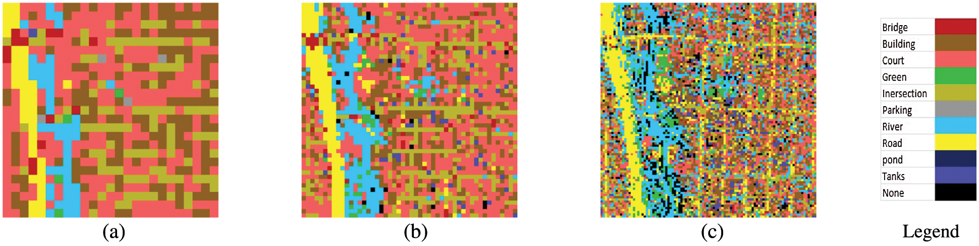
Figure 12: Using the proposed FC layers model that be trained using the UC merced land use dataset (a) 200 × 200 blocks (b) 100 × 100 blocks (c) 50 × 50 blocks

Figure 13: Using the proposed SVM model that be trained using the UC merced land use dataset (a) 200 × 200 blocks (b) 100 × 100 blocks (c) 50 × 50 blocks

Figure 14: Using the proposed FC layers model that be trained using the SIRI-WHU dataset (a) 200 × 200 blocks (b) 100 × 100 blocks (c) 50 × 50 blocks

Figure 15: Using the proposed SVM model that be trained using the SIRI-WHU dataset (a) 200 × 200 blocks (b) 100 × 100 blocks (c) 50 × 50 blocks
As shown from visual inspection of the classified scene, the trained models using the SIRI-WHU datasets result in very low correct predictions. It can be considered that because the used big scene's spatial resolution is higher than the used dataset images’ spatial resolution. There are also some classes in this scene that don't exist in the used dataset images. Using the UC Merced land use datasets, the trained models result in accepted correct predictions, especially in roads and river classes. On the other hand, the FC model results in a little better accurate predictions than the SVM model. It can be considered that because the used big scene's spatial resolution is near to the used dataset images’ spatial resolution where the used scene has 1 square feet & 6 square inches spatial resolution. The UC Merced land use dataset images have 1 square foot spatial resolution. All of the scene classes, except pond class, exist in the used dataset images. The source of the UC Merced land use dataset images is similar to the source of the big scene which these dataset images are elicited from big images gathered from the National Map Urban Area Imagery combination in the USGS library for different urban areas around the USA that captured by an aerial camera. The big scene is taken from the USGS library of remote sensing images that was captured by an aerial camera. The CNNs give high edge detection, and then it explains to us the good correct predictions for roads and rivers. Dividing this big scene into 50 × 50 blocks gives better predictions by visual inspection because the 50 × 50 blocks are considered more specified images. Even if the training and testing with low spatial resolution remote sensing images datasets give greater OA than the training and testing with high spatial resolution remote sensing images datasets. Still, it is preferred to train classification models using higher spatial resolution remote sensing images datasets to get accepted correct predictions ratio when using these trained models to predict any other scenes. On the other hand, it is necessary to use trained classification models using dataset images taken from a similar source of the scenes, which require predictions for its classes, to get accepted correct predictions ratio.
This paper proposed two efficient methods for classifying remote sensing images. These proposals consisted of two stages; extracting convolution features and training the classifiers using these extracted features. Convolution features extraction was done by concatenating two convolution models’ outputs, with ImageNet pre-trained weights, after transfer learning; the ResNet 50 model, and the DenseNet 169 model. These elicited features were used as input features for two classifiers; the FC and the SVM classifiers. The experimental results demonstrated that the proposed methods had high accuracy and revealed their superiority to the other classifiers. The proposed models with their trained weights were used to predict a big scene's classes. The trained weights with the UC Merced land use dataset resulted in accepted correct predictions, but the trained weights with the SIRI-WHU dataset resulted in very limited predictions. This result revealed that it is necessary to train the remote sensing images classifiers with dataset images taken from the similar source of scenes that require predictions for its classes. On the other hand, it is preferred to train models with high spatial resolution dataset images.
Acknowledgement: The authors would like to thank the Deanship of Scientific Research, Taif University Researchers Supporting Project Number (TURSP-2020/239), Taif University, Taif, Saudi Arabia for supporting this research work.
Funding Statement: This study was funded by the Deanship of Scientific Research, Taif University Researchers Supporting Project Number (TURSP-2020/239), Taif University, Taif, Saudi Arabia.
Conflicts of Interest: The authors declare that they have no conflicts of interest to report regarding the present study.
1. M. Bowling, J. Furnkranz, T. Graepel and R. Musick, “Machine learning and games,” Machine Learning, vol. 63, no. 3, pp. 211–215, 2006. [Google Scholar]
2. K. H. Kim and S. J. Kim, “Neural spike sorting under nearly 0-dB signal-to-noise ratio using nonlinear energy operator and artificial neural-network classifier,” IEEE Transactions on Medical Engineering, vol. 47, no. 10, pp. 1406–1411, 2000. [Google Scholar]
3. X. Liu, J. Yu, W. Song, X. Zhang, L. Zhao et al., “Remote sensing image classification algorithm based on texture feature and extreme learning machine,” Computers, Materials & Continua, vol. 65, no. 2, pp. 1385–1395, 2020. [Google Scholar]
4. W. Rawat and Z. Wang, “Deep convolutional neural networks for image classification: A comprehensive review,” Neural Computation, vol. 29, no. 9, pp. 2352–2449, 2017. [Google Scholar]
5. K. A. AlAfandy, H. Omara, M. Lazaar and M. Al Achhab, “Artificial neural networks optimization and convolution neural networks to classifying images in remote sensing: A review,” in Proc. of the 4th Int. Conf. on Big Data and Internet of Things (BDIoT’19), Rabat, Morocco, 2019. [Google Scholar]
6. G. Ahmad, S. Alanazi, M. Alruwaili, F. Ahmad, M. A. Khan et al., “Intelligent ammunition detection and classification system using convolutional neural network,” Computers, Materials & Continua, vol. 67, no. 2, pp. 2585–2600, 2021. [Google Scholar]
7. P. Liu, K. R. Choo, L. Wang and F. Huang, “SVM or deep learning? a comparative study on remote sensing image classification,” Soft Computing, vol. 21, no. 23, pp. 7053–7065, 2016. [Google Scholar]
8. Y. Guo, X. Jia and D. Paull, “Effective sequential classifier training for SVM-based multitemporal remote sensing image classification,” IEEE Transactions on Image Processing, vol. 27, no. 6, pp. 3036–3048, 2018. [Google Scholar]
9. C. Sukawattanavijit, J. Chen and H. Zhang, “GA-SVM algorithm for improving land-cover classification using SAR and optical remote sensing data,” IEEE Geoscience and Remote Sensing Letters, vol. 14, no. 3, pp. 284–288, 2017. [Google Scholar]
10. Y. Liu, B. Zhang, L. Wang and N. Wang, “A self-trained semisupervised SVM approach to the remote sensing land cover classification,” Computers & Geosciences, vol. 59, pp. 98–107, 2013. [Google Scholar]
11. G. P. Petropoulos, C. Kalaitzidis and K. P. Vadrevu, “Support vector machines and object-based classification for obtaining land-use/cover cartography from Hyperion hyperspectral imagery,” Computers & Geosciences, vol. 41, pp. 99–107, 2012. [Google Scholar]
12. M. Wang, X. Zhang, X. Niu, F. Wang and X. Zhang, “Scene classification of high-resolution remotely sensed image based on ResNet,” Journal of Geovisualization and Spatial Analysis, vol. 3, no. 2, pp. 16–25, 2019. [Google Scholar]
13. Y. Jiang, Y. Li and H. Zhang, “Hyperspectral image classification based on 3-D separable ResNet and transfer learning,” IEEE Geoscience and Remote Sensing Letters, vol. 16, no. 12, pp. 1949–1953, 2019. [Google Scholar]
14. S. Natesan, C. Armenakis and U. Vepakomma, “ResNet-based tree species classification using UAV images,” International Archives of the Photogrammetry, Remote Sensing & Spatial Information Sciences, vol. XLII, pp. 475–481, 2019. [Google Scholar]
15. J. Yang, Y. Zhu, B. Jiang, L. Gao, L. Xiao et al., “Aircraft detection in remote sensing images based on a deep residual network and super-vector coding,” Remote Sensing Letters, vol. 9, no. 3, pp. 229–237, 2018. [Google Scholar]
16. L. Xu and Q. Chen, “Remote-sensing image usability assessment based on ResNet by combining edge and texture maps,” IEEE Journal of Selected Topics in Applied Earth Observations and Remote Sensing, vol. 12, no. 6, pp. 1825–1834, 2019. [Google Scholar]
17. Y. Tao, M. Xu, Z. Lu and Y. Zhong, “DensNet-based depth-width double reinforced deep learning neural network for high-resolution remote sensing images per-pixel classification,” Remote Sensing, vol. 10, no. 5, pp. 779–805, 2018. [Google Scholar]
18. G. Yang, U. B. Gewali, E. Ientilucci, M. Gartley and S. T. Monteiro, “Dual-channel DenseNet for hyperspectral image classification,” in Proc. of IGARSS 2018 IEEE Int. Geoscience and Remote Sensing Symposium, Valencia, Spain, pp. 2595–2598, 2018. [Google Scholar]
19. J. Zhang, C. Lu, X. Li, H. Kim and J. Wang, “A full convolutional network based on DenseNet for remote sensing scene classification,” Mathematical Biosciences and Engineering, vol. 6, no. 5, pp. 3345–3367, 2019. [Google Scholar]
20. K. A. AlAfandy, H. Omara, M. Lazaar and M. Al Achhab, “Using classic networks for classifying remote sensing images: Comparative study,” Advances in Science, Technology and Engineering Systems Journal (ASTESJ), vol. 5, no. 5, pp. 770–780, 2020. [Google Scholar]
21. K. A. AlAfandy, H. Omara, M. Lazaar and M. Al Achhab, “Investment of classic deep CNNs and SVM for classifying remote sensing images,” Advances in Science, Technology and Engineering Systems Journal (ASTESJ), vol. 5, no. 5, pp. 652–659, 2020. [Google Scholar]
22. M. El Mamoun, Z. Mahmoud and S. Kaddour, “SVM model selection using PSO for learning handwritten arabic characters,” Computers, Materials & Continua, vol. 61, no. 3, pp. 995–1008, 2019. [Google Scholar]
23. B. W. Heumann, “An object-based classification of mangroves using a hybrid decision tree-support vector machine approach,” Remote Sensing, vol. 3, no. 11, pp. 2440–2460, 2011. [Google Scholar]
24. K. He, X. Zhang, S. Ren and J. Sun, “Deep residual learning for image recognition,” in Proc. of 2016 IEEE Conf. on Computer Vision and Pattern Recognition (CVPR), Las Vegas, NV, USA, pp. 770–778, 2016. [Google Scholar]
25. G. Huang, Z. Liu, L. Maaten and K. Q. Weinberger, “Densely connected convolutional networks,” in Proc. of 2017 IEEE Conf. on Computer Vision and Pattern Recognition (CVPR), Honolulu, HI, USA, pp. 2261–2269, 2017. [Google Scholar]
26. W. Li, H. Fu, L. Yu and A. Cracknell, “Deep learning based oil palm tree detection and counting for high-resolution remote sensing images,” Remote Sensing, vol. 9, no. 1, pp. 22–34, 2017. [Google Scholar]
27. G. Banko, “A review of assessing the accuracy of classifications of remotely sensed data and of methods including remote sensing data in forest inventory,” in Int. Institution for Applied Systems Analysis (IIASA), Laxenburg, Austria, IR-98-081, 1998. [Google Scholar]
28. K. A. Al-Afandy, E. M. EL-Rabaie, F. E. Abd El-Samie, O. S. Faragallah, A. ELmhalaway et al., “A comparative study for color systems used in the DCT-DWT watermarking algorithm,” Advances in Science, Technology and Engineering Systems Journal (ASTESJ), vol. 1, no. 5, pp. 42–49, 2016. [Google Scholar]
29. Y. Yang and S. Newsam, “Bag-of-visual-words and spatial extensions for land-use classification,” in Proc. of the 18th ACM SIGSPATIAL Int. Conf. on Advances in Geographic Information Systems, San Jose California, USA, pp. 270–279, 2010. [Google Scholar]
30. B. Zhao, Y. Zhong, G. Xia and L. Zhang, “Dirichlet-derived multiple topic scene classification model for high spatial resolution remote sensing imagery,” IEEE Transactions on Geoscience and Remote Sensing, vol. 54, no. 4, pp. 2108–2123, 2016. [Google Scholar]
31. J. L. Dwyer, “Remotely sensed data available from the US geological survey EROS data center,” in Earth Science Satellite Remote Sensing, J. J. Qu et al., (Eds.Berlin, Heidelberg: Springer, pp. 18–51, 2006. [Google Scholar]
32. E. Bisong, “Building Machine Learning and Deep Learning Models on Google Cloud Platform: A Comprehensive Guide for Beginners,” Berkeley, CA: Apress, pp. 1–64, 2019. [Google Scholar]
33. O. Russakovsky and L. Fei-Fei, “Attribute learning in large-scale datasets,” in Proc. of European Conf. on Computer Vision, Heraklion Crete, Greece, pp. 1–14, 2010. [Google Scholar]
 | This work is licensed under a Creative Commons Attribution 4.0 International License, which permits unrestricted use, distribution, and reproduction in any medium, provided the original work is properly cited. |