Computers, Materials & Continua DOI:10.32604/cmc.2022.022648
Article

Design of Machine Learning Based Smart Irrigation System for Precision Agriculture

Khalil Ibrahim Mohammad Abuzanouneh1, Fahd N. Al-Wesabi2, Amani Abdulrahman Albraikan3, Mesfer Al Duhayyim4, M. Al-Shabi5, Anwer Mustafa Hilal6, Manar Ahmed Hamza6,*, Abu Sarwar Zamani6 and K. Muthulakshmi7

1Department of Information Technology, College of Computer, Qassim University, Al-Bukairiyah, 52571, Saudi Arabia
2Department of Computer Science, King Khalid University, Muhayel Aseer, 62529, Saudi Arabia & Faculty of Computer and IT, Sana'a University, Sana'a, 61101, Yemen
3Department of Computer Science, College of Computer and Information Sciences, Princess Nourah Bint Abdulrahman University, Riyadh, 11564, Saudi Arabia
4Department of Natural and Applied Sciences, College of Community - Aflaj, Prince Sattam bin Abdulaziz University, Al-Kharj, 16278, Saudi Arabia
5Department of Management Information System, College of Business and Administrative, Taibah University, Medina, 42353, Saudi Arabia
6Department of Computer and Self Development, Preparatory Year Deanship, Prince Sattam bin Abdulaziz University, Al-Kharj, 16278, Saudi Arabia
7Department of Electronics and Communication Engineering, Dr. N. G. P Institute of Technology, Coimbatore, 641048, India
*Corresponding Author: Manar Ahmed Hamza. Email: ma.hamza@psau.edu.sa
Received: 14 August 2021; Accepted: 29 September 2021

Abstract: Agriculture 4.0, as the future of farming technology, comprises numerous key enabling technologies towards sustainable agriculture. The use of state-of-the-art technologies, such as the Internet of Things, transform traditional cultivation practices, like irrigation, to modern solutions of precision agriculture. To achieve effective water resource usage and automated irrigation in precision agriculture, recent technologies like machine learning (ML) can be employed. With this motivation, this paper design an IoT and ML enabled smart irrigation system (IoTML-SIS) for precision agriculture. The proposed IoTML-SIS technique allows to sense the parameters of the farmland and make appropriate decisions for irrigation. The proposed IoTML-SIS model involves different IoT based sensors for soil moisture, humidity, temperature sensor, and light. Besides, the sensed data are transmitted to the cloud server for processing and decision making. Moreover, artificial algae algorithm (AAA) with least squares-support vector machine (LS-SVM) model is employed for the classification process to determine the need for irrigation. Furthermore, the AAA is applied to optimally tune the parameters involved in the LS-SVM model, and thereby the classification efficiency is significantly increased. The performance validation of the proposed IoTML-SIS technique ensured better performance over the compared methods with the maximum accuracy of 0.975.

Keywords: Automatic irrigation; precision agriculture; smart farming; machine learning; cloud computing; decision making; internet of things

1  Introduction

The effects of global warming and growing droughts lead to the scarcity on the continuous availability of water resource. It has a risk for water crises and food security due to the predictable rise from population to 9.8 billion in 2050. As irrigation is a substantial user of freshwater, excess resources from this region can have significant effects on food security [1]. Subsequently, for increasing the performance of water usage by the accuracy irrigation, the combination of cutting edge technologies like control strategies for optimization & prediction, IoT, identification, irrigation management are utilized by considering the dependence in the environment and improve accuracy of irrigation system [2,3]. Accuracy irrigation system performs a major part in offering substantial contribution to the food production and decrease the stress faced by the farmer. Thus, there is requirement for accurately designing an irrigation system which could adapt, deliver and predict the proper quantity of water to the crops when and where it is required regarding the altering dynamics of the plant, weather, and soil [4].

Information and communication technology (ICT) has presented to the sustained management of water in agriculture. The placement of WSN from crops via IoT technology and the remote management of data using CC has enabled huge monitoring of agricultural parameters that create a huge number of data [5,6]. Additionally, the democratization of IoT technology to monitor weather and soil parameters are enabling extensive distribution of water saving tool in home context [7]. But, the continual modernization of irrigation system should execute equipment's which enables automatic scheduling of irrigation. It should have sensors for providing distinct variables. Conventionally, these variables are compared with environmental conditions and provide the data regarding whole crop water necessities by means of weather station and soil water status/volumetric content, indicates water availability for the plant. Mostly, they utilize soil variable sensors for dielectric properties, as they are flexible and cheap [8], though its accurate operation needs complex calibration, considering aspects like water salinity, soil texture & structure, and temperature also the spatial variability of the soil condition. Other sensors like infrared radiometers (IR), satellites, multispectral & thermal cameras, are utilized for estimating water crop needs. For handling this difficult problem, several sensor based smart irrigation systems using mobile applications are implemented at distinct times. As in previous study, the temperature, input variables humidity, light intensity, and soil moisture, have been utilized, and a decision of watering plants are created based on fuzzy logic (FL) [9]. A similar FL was employed for several healthcare schemes, where the utilization of biosensors assists in monitoring blood pressure, temperature, infection status of the wound, and oxygen.

Recently, with growing computer processors, many artificial intelligences based approaches like LSSVM, ANN, NF-SC, and NF-FCM are established as beneficial methods for modelling difficult problems. These modules have been extended for simulating and solving the challenges in distinct regions because of a huge amount of efficient variables, interaction among the higher uncertainty, parameters, and difficulty of the solution. Several applications of AI model have been stated until now in the region of irrigation, for example, evaluation of the nutrient and water distribution regularity in the soil, evaluating soil moisture distribution, simulates water distribution regularity of sprinkler irrigation system. Distinct methods are utilized for water need estimation in automated irrigation system deepening upon ML, ANN, and SVR methods are extensively utilized to DSS growth. In KNN and AdaBoost methods have been related to ANN to evaluation of potato water necessities. The researchers in related SVR to MARS and M5Tree in modelling ETo. GA and RFR are utilized for water need estimations.

This paper design an IoT and ML enabled smart irrigation system (IoTML-SIS) for precision agriculture. The proposed IoTML-SIS technique senses the parameters of the farmland and makes appropriate decisions for irrigation. The proposed IoTML-SIS model allows different IoT based sensors for soil moisture, humidity, temperature sensor, and light data collection. In addition, artificial algae algorithm (AAA) with least squares-support vector machine (LS-SVM) model is employed for the classification process to determine the need for irrigation. For optimally adjusting the parameters involved in LS-SVM method, AAA is employed and thereby the classification performance gets improved. For ensuring the improved classification efficiency of the presented IoTML-SIS technique, extensive experimental analysis is carried out and the results are examined interms of different aspects.

2  Literature Review

Ahmed et al. [10] presented the implementation and design of smart irrigation scheme with help of IoT technique that is utilized to automate the irrigation procedure from agricultural fields. It can be predictable that scheme will make the best change for the farmers to irrigate their field effectively, and eliminate the field in watering, that can stress the plant. The established scheme is classified into 3 portions: user side, sensing side, and cloud side. They utilized Microsoft Azure IoT Hub as a fundamental framework for coordinating the communication among the 3 sides. Blasi et al. [11] improved the irrigation procedure and provides irrigation water to the maximum range using AI for constructing smart irrigation schemes. The sensor measures the temperature & humidity from the soil each 10 min. It can be prevented the automated irrigation procedure when the humidity was higher and allows it when the humidity was lower. The smart automated irrigation scheme is made by DT method that is an ML technique which trains the scheme based on gathered data for creating the module which would be utilized for examining and predicting the residual data.

The projected solution would be established by developing a distributed WSN, where all the regions of farm will be enclosed with several sensor models that would be transferring data on a standard server. The ML method would assist prediction of the irrigation pattern depending upon weather conditions and crops. Hence, a sustained method for irrigation is given in [12]. Hassan-Esfahani et al. [13] introduced a modelling method for an optimum water distribution relation to maximize irrigation regularity and minimize yield decrease. Local weather data, field measurements, and Landsat images have been utilized for developing a module which defines the field condition by a soil water balance method. This method has predicted the elements of soil water balance and optimization of water allocation module. Every module includes 2 sub components which consider 2 purposes. The optimization sub module utilizes GA for identifying optimum crop water application rates depending upon sensitivity, crop type, and growth stage to water stress.

In Shen et al. [14], the water saving irrigation scheme for winter wheat depending upon the DSSAT module and GA is improved for distinct historical years (1970–2017). Hence, a decision making technique to defining either for irrigating development phase of winter wheat was established by SVM method depending upon quantity of precipitations in the initial phase of winter wheat and the quantity of irrigations. Navarro-Hellín et al. [15] allow a closed loop control system for adapting the DSS for estimation errors and local perturbations. The 2 ML methods, ANFIS & PLSR, are presented as reasoning engine of this SIDSS. Cardoso et al. [16] presented ML methods using the aim of forecasting the appropriate time of day for water administration to agricultural fields. Using higher quantity of data formerly gathered by WSN in agricultural fields it can examine techniques that permit for predicting the optimal time to water management for eliminating scheduled irrigation which always results in excess of water being the major goal of the scheme for saving these similar natural resources.

For adapting water management, ML methods have been investigated for predicting the optimal time of day for water administration [17]. The research methods like DT, SVM, RF, and NN are the most attained outcomes was RF, giving 84.6% accuracy. Also the ML solution, a technique was established for calculating the quantity of water required for managing the field in analyses. Munir et al. [18] used a smart method that can professionally utilize ontology for making 50% of decision and another 50% of decision based on sensor information values. The decision in ontology and sensor value cooperatively becomes the source of last decision that is the outcome of an ML method KNN. This technique avoids the overburden of the IoT server for processing data however it decreases the latency rate. The goal of [19] is the research of many learning methods for determining the goodness and error comparative for expert decisions. The 9 orchards have been verified in 2018 by LR, RFR, and SVR approaches as engine of the IDSS presented. In Abioye et al. [20], an enhanced data driven and monitoring modelling of the dynamics of variables affected the irrigation of mustard leaf plants is proposed.

3  The Proposed Model

Fig. 1 demonstrates the overall working process of the proposed IoTML-SIS model. This presented framework of IoT has perception layer, application layer, processing layer, and transport layer. The perception layer is called as physical layer that implies it can be sensor to the data assembling. It has been senses temperature, soil moisture, and humidity in air. The transport layer was the source of transporting sensed information gathered formerly to processing layer via networks like LAN, wireless, 2G, and 3G. The processing layer scrutinizes, saves, and developments large number of data that comes in transport layer. It uses techniques like edge computing, databases, and CC. The application layer is to provide application particular service for end user.

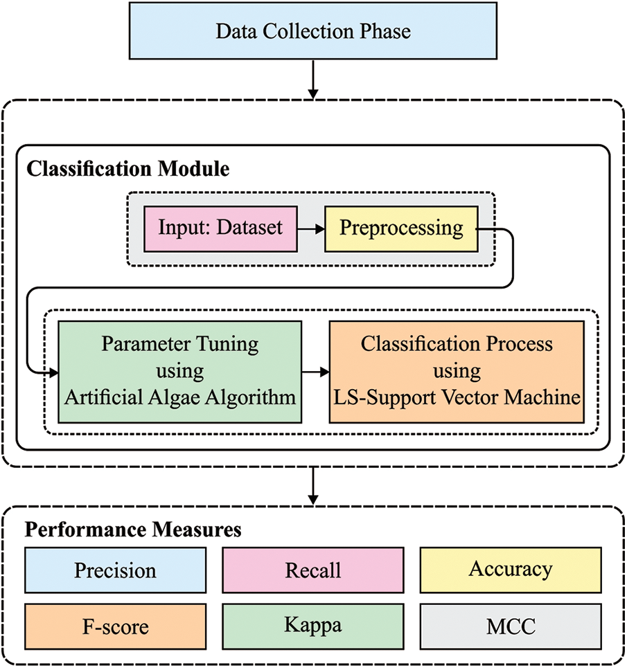
Figure 1: Overall process of IoTML-SIS model

3.1 Sensor Data

Initially, data is collected by the sensors. Temperature, Soil moisture, and humidity data are gathered in this stage. The perception layer contains microcontroller, actuator, and sensor. Rest is the portion of residual 3 layers. Processing and Transport layers cooperatively offer schedules to water crops, other suggestions, and their supervision. Afterward collecting the data, the following phase is for collecting data in data centres for analysis. The complete design investigation of the physical component utilized is proposed in the figure. Every element is without trouble existing from market and inexpensive. Hence, the device that exists placed from the real environment could be created easily existing. These implantable devices have the layer of sensor utilized that is, light, moisture, and humidity sensors. The microcontroller set from Arduino board attains analog signal in this sensor, and for all thirty seconds, this value is transported to data centre via GSM model SIM808. The last result from this decision making procedure could be visualized with the client completely by an android application, then the client could direct this system actuator, and later, water is discharged in the valve/closed.

3.1.1 HL-69 Soil Hygrometer Sensor

For detecting humidness of the soil, they utilized HL-69 soil hygrometer moisture sensors. The fundamental objective to utilize for the HL-69 soil hygrometer moisture sensor is given an optimal reading compared to another soil moisture sensor. The sensors are utilized to monitor real world soil moisture of plants from tunnel farm. The voltage of sensors output changes consequently to water contents from soil. It has few main aspects of HL-69 soil hygrometer sensors. When the soil moisture was higher, next the output voltage reduces, however when the soil was dry, afterward the output voltage rises. The hygrometer soil moisture sensors give an analog signal as output that should be transformed to digital using Arduino. These sensors have electronic board and 2 pads which detecting the water contents. LM393 comparator chip is placed on electronic board. It has green and red lights; red light displays the power indicators, and green light displays the digital switching output indicators.

3.1.2 AM2302 DHT11 Sensor

The DHT22 sensor is standard temperature-humidity sensors which is utilized for determining the humidness and temperature in air. The DHT22 sensor is composed of thermistor and humidity sensor. It has few major aspects of the DHT22 sensor that is given by: the cost of DHT22 sensor is lower. The Input or Output voltage to DHT22 sensors are among [3, 5 V]. When apply for the data, the maximal present usage in the transformation is 2.5 mA. DHT22 sensor has four pins alongside 0.1 spacing among them. The body sizes of DHT22 sensor is around 15.1∗25∗7.7mm.

3.1.3 BH1750 FVI Light Sensor

BH1750 is a standard digital light sensor which could define the light intensities. BH1750 is a calibrated digital light sensor, and it could measure smaller trace of light and could transform to a 16-digit numerical value. It can be generally utilized from mobile phones for exploiting the screen brightness depending upon lighting environment. BH1750 measure the light intensities at the range of [0–65,535] lux (L). It has few main aspects of BH1750 sensor that is given by: the chip of BH1750 sensor has BH1750FVI. The power supply of BH1750 sensor was [3.3–5 V]. The BH1750 sensor was in-built 16 bits AD converter which transforms detection of light to 16 digit numerical values.

3.2 LS-SVM Based Classification

Once the sensor related data are collected, they are fed into the LS-SVM model to perform classification process. SVM is determined as a new ML and provides maximal benefit for solving the problems such as over fitting and local optimal. SVM module is efficient and utilized in several applications such as pattern recognition, regression analysis, and so on. LS-SVM was expanded module of regular SVM that transforms a quadratic programming (QP) problem to linear equation, fast solution speed, and strong real time functions could be obtained. Consider D={(xu,yu)|u=1,2,3,…,N} represents training data, whereas xi denotes input and yu indicates outcome. In the event of non-linear regression, LS-SVM is labelled by:

y(x)=ωTφ(xu)+b+eu,(1)

whereas ω stands for weight vector, φ(xu) indicates non-linear function, b implies the deviation, and eu signifies appropriate error [21] that is an error amongst the actual trained and computed outputs of the data group u. ω and b is attained in the provided optimization problems.

minJ(w,e)=12ωTω+γ12∑u=1N⁡eu2,(2)

Eq. (2) meet the constraints:

yi=ωTφ(xu)+b+eu,u=1,2,3,…,N,(3)

In Eq. (2), a main part is to alter the weight and decrease huge weights, and later succeeding part denotes training error. Eq. (2), determines the Lagrange function L:

L(w,b,e,α)=I(w,e)−∑u=1Nαu{ωTφ(xu)+b+eu−yu},(4)

In Eq. (4), αu denotes Lagrange multiplier and γ indicates penalty parameter that estimates the complexity of LS-SVM methods like y(x) and trained error. Eq. (4) is employed for attaining the partial derivatives of w,b,e and αu and turn into 0, and attain an optimization state.

{∂L∂w=0→w=∑u=1Nαuφ(xu)∂L∂b=0→∑u=1Nαu=0∂L∂eu=0→αu=Λeu∂L∂αu=0→ωTφ(xu)+b+eu−yu=0(5)

The ω is eliminated and the LS-SVM regression module was attained.

y(x)=∑u=1NαuK(x,xu)+b,(6)

where K(x,xu) implies the kernel function, that is defined as follows

K(x,xu)=exp(−||x−x2||22σ2),(7)

where σ2 denotes kernel variable. Penalty variable γ and kernel variables σ2 are limited by the accuracy of LS-SVM method. The generalized ability of a method could be enhanced by decreasing γ, simultaneously training error enhances. Since the kernel variable is minimal, and later the model's complexity is enhanced, if kernel variable is high, later it outcomes from lack of learning. Therefore, a substantial γ and σ2 measures are the major goal for attaining remarkable effectiveness.

3.3 Parameter Optimization Using AAA

For optimally adjusting the parameters γ and σ involved in the LS-SVM method, AAA is employed, and thereby the classification performance gets improved. Here, 10-fold cross validation approach is employed and a fitness function is derived based on the error rate, as given below.

fitness=(∑i=1K⁡testErrori)/k(8)

where testErrori stands for the average test error rates obtained by the LS-SVM model. The AAA provides an optimal solution by the stimulation of algae feature [22]. Related to actual algae, AAA moves to the light source for photosynthesis using the application of helical swimming, and it is adaptable to the whole environment, that is appropriate to adjust the primary species and recreated by mitotic separation. Henceforth, the AA method has “helical movement”, “evolutionary process” and “adaptation”. Everyone is determined as a group of algal cells that lives in set (Eqs. (9) and (10)). If a single algal cell is categorized for generating 2 novel algal cells that are nearby in nature and the additional classification generates four cells. The algal colony act as a single cell, that is moved together, and cells in a colony pass away in unfavorable situation. The physical applications like shear force share the colonies and parts that are handled as novel colonies. It is existing at an optimal point is named a colony of optimal and has optimum algal cells.

PopulationofAlgalcolony=[x11⋯x1D⋮⋱⋮xN1⋯xND](9)

ithalgalcolony=[xi1,xi2…xiD](10)

Whereas xij denotes algal cell in jth dimensional of ith algal colony.

With sufficient nutrient case the algal colony attains sufficient light, it starts to improve and regenerated as two novel algal cells in time t, that is comparable to real mitotic separation. However, the algal colony doesn't adapt to sufficient light and gradually passes away. The development kinetics of algal colony is defined by Monod method as provided whereas, μ represents specific growth rate, μmax indicates high growth rate, S denotes nutrient focus that is called as fitness value (ft(xi)) at time t and K represents substrate half saturation constant of algal colony. μmax is considered as 1. K is defined as a growth rate at half nutrient state of algal colony at time t. The size of ith algal colony from time t+1 in Monod function as provided by Eq. (11):

Git+1=μitGiti=1,2,…N(11)

Whereas Git denotes size of ith algal colony in time t, N indicates algae colony amount. Algal colony provides optimal solutions to develop maximal nutrients since it achieves an optimum one. For algal cells of smaller algal colonies in an evolution procedure, algal cell of main algal colony is equated by Eqs. (12)–(14).

biggestt=maxGiti=1,2,…N(12)

smallestt=Giti=1,2,…N(13)

smallestmt=biggestmtm=1,2,…N(14)

Whereas D represents dimension, high the maximal algal colony and small is the minimal one.

In AAA, algal colony is organized based on sizes in time t. From arbitrarily determining dimensional, algal cell of minimal algal colony died and algal cell of higher colony is simulated. Fig. 2 exhibited the process flow of AAA. The algal colony is not appropriate for developing in sufficient environment, that tries to accept in a platform and lastly, the main species are altered. Adaptation is determined as procedure in which inadequate algal colony imitates the largest algal colony. It is decided with the modification in starvation level in this module. Firstly, the starvation value is 0 to entire artificial alga. Starvation value is improved by time t, if an algal cell attains insufficient light source.

stravingt=maxAiti=1,2,…N(15)

stravingt+1=stravingt+(biggestt−stravingt)×rand(16)

whereas Ait denotes starvation measure of ith algal colony in time t, stravingt represents algal colony using maximal starvation value at time t. The adaptation variable (Ap) calculates either the modification task may be utilized at time t or not. Ap refer the constant from zero and one.

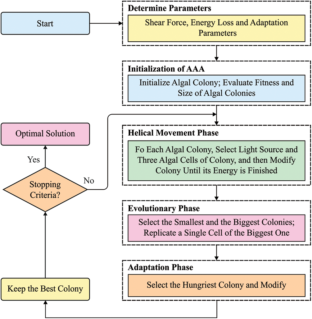
Figure 2: Process flow of AAA

Colonies swim & Algal cells attempt to exist in adjacent water surfaces because of the sufficient light for survival rate. It swims in helical architecture in liquid by flagella. The movement of algal cells is distinct. As it is a friction surface, the evolution of algal cells is established quickly and frequency of helical actions are improved by enhancing the local search capability. The power of algal cell in time t is equivalent to amount of nutrients spent in the time. Henceforth, maximal algal cell is nearby to surface, it has high energy level that moves in the liquid. Later, friction surface turns into minimal and motion distance of liquid becomes expanded consequently. Therefore, the global search potency was improved. Thus, it moves to the lowest energy proportion. The motion of an algal cell was executed helically. Likewise, it can be spherical in shape, and volume is denoted by size. Therefore, friction surface is deliberated as surface area of hemisphere (Eqs. (17) and (18)).

τ(xi)=2πr2(17)

τ(xi)=2π(3Gi4π3)2(18)

where τ(xi) denotes friction surface. The three dimension structure for helical motion of an algal cell is calculated in arbitrary way. It offers linear motion in Eq. (19) and residual 2 dimensional give angular effort from Eqs. (20) and (21). Eq. (20) is employed to 1 dimension problem and algal cell is moved in one way. In event of 2 dimension problems, algal movement is denoted by sinusoidal, and so the Eqs. (19) and (21) were employed. For huge dimensions, algal motion is executed helically and Eqs. (19)–(21) are utilized. Friction surface and distance to light source estimates the step size of every motion:

ximt+1=ximt+(xjmt−ximt)(Δ−τi(xi))p(19)

xikt+1=xikt+(xjkt−xikt)(Δ−τi(xi))cosα(20)

xilt+1=xilt+(xjlt−xilt)(Δ−τi(xi))sinβ(21)

whereas Xikt, Xilt and Ximt are x, y and z coordinate point of ith algal cell in time t; α, β∈[0,2π]; p∈[−1,1]; Δ indicates shear force; τi(xi) represents friction surface area of ith algal cell.

4  Performance Validation

This section validates the performance of the presented IoML-SIS technique. The presented model is tested using three sensor data namely soil moisture, temperature, and humidity. The dataset holds five class labels namely high needed, needed, average, not needed, and highly not needed. The data ranges of the sensor data and its respective labels are given in Fig. 3.

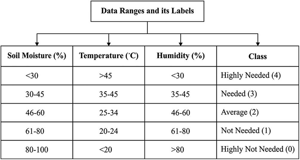
Figure 3: Dataset descriptions

A set of confusion matrices generated by the IoTML-SIS technique under different test runs are given in Fig. 4. On the execution run-1, the IoTML-SIS technique has classified 90 samples under Highly Not Needed, 92 samples under Not Needed, 92 samples under average, 91 samples under Needed, and 93 images under Highly Needed. Meanwhile, on the execution run-2, the IoTML-SIS approach has ordered 91 samples under Highly Not Needed, 93 samples under Not Needed, 94 samples under average, 93 samples under Needed, and 94 images under Highly Needed.

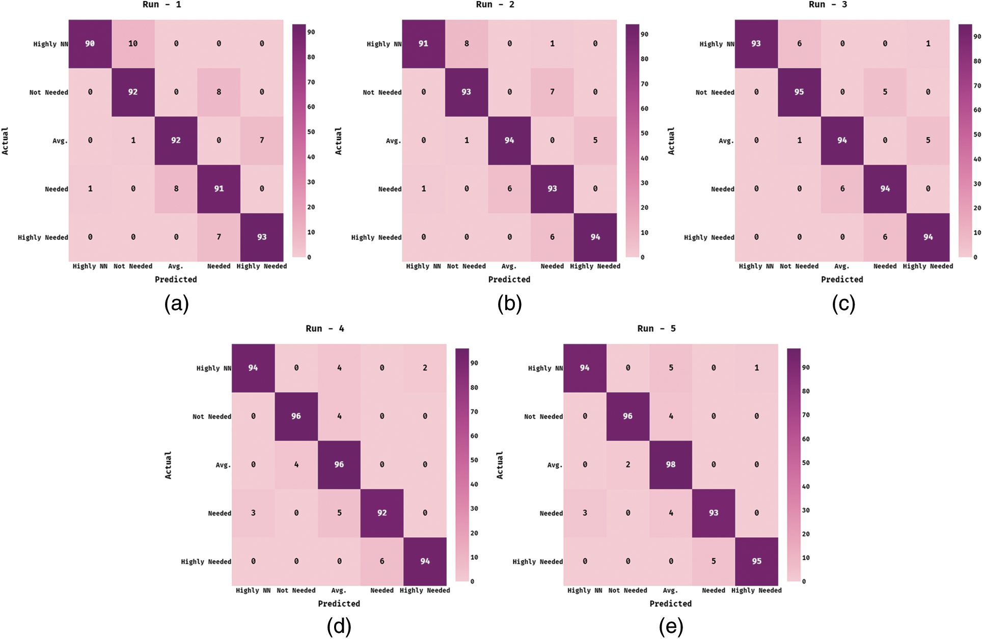
Figure 4: Confusion matrix of proposed IoTML-SIS method on different runs (a) Run-1, (b) Run-2, (c) Run-3, (d) Run-4, and (e) Run-5

Eventually, on the execution run-3, the IoTML-SIS method has ordered 93 samples under Highly Not Needed, 95 samples under Not Needed, 94 samples under average, 94 samples under Needed, and 94 images under Highly Needed. Concurrently, on the execution run-4, the IoTML-SIS manner has classified 94 samples under Highly Not Needed, 96 samples under Not Needed, 96 samples under average, 92 samples under Needed, and 94 images under Highly Needed. Lastly, on the execution run-5, the IoTML-SIS methodology has ordered 94 samples under Highly Not Needed, 96 samples under Not Needed, 98 samples under average, 93 samples under Needed, and 95 images under Highly Needed.

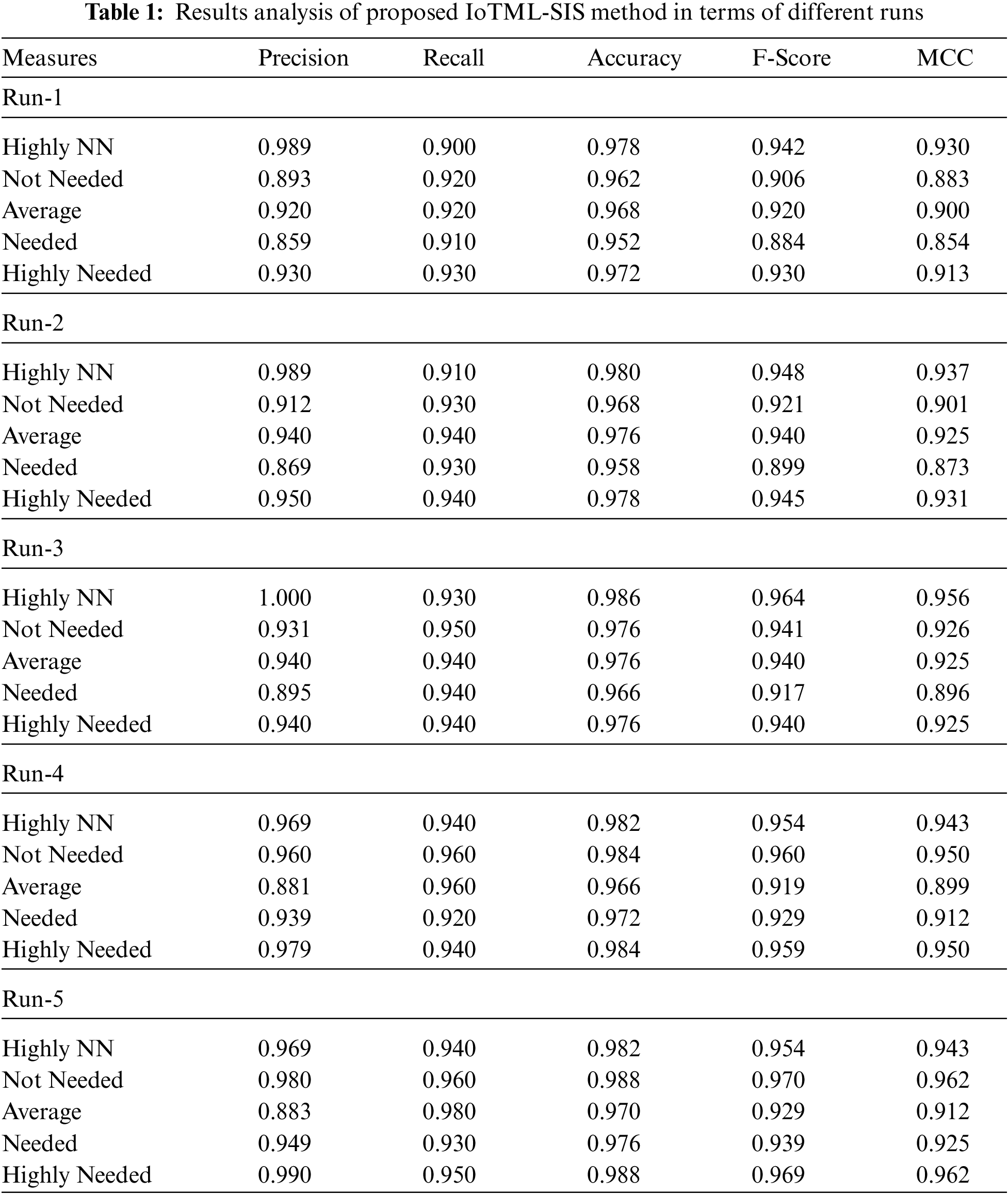
A detailed classification results analysis of the IoTML-SIS technique takes place interms of different measures in Tab. 1. Besides, the results are examined under varying number of runs. The experimental results stated that the IoTML-SIS technique has accomplished effective outcomes under all the applied runs.

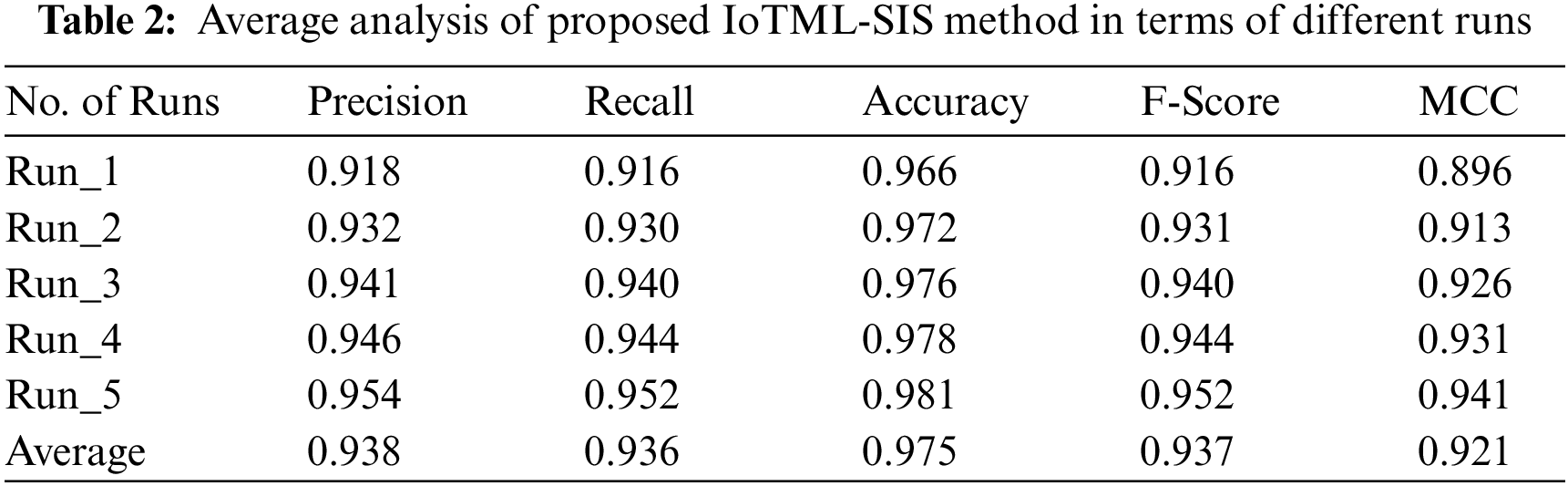
Tab. 2 offers a brief average results analysis of the IoTML-SIS technique interms of distinct measures. The experimental outcomes showcased that the presented IoTML-SIS technique has obtained maximum performance. For instance, the IoTML-SIS technique has attained an average precision of 0.918, recall of 0.916, accuracy of 0.966, F-score of 0.916, and MCC of 0.896. Simultaneously, the IoTML-SIS manner has achieved an average precision of 0.932, recall of 0.930, accuracy of 0.972, F-score of 0.931, and MCC of 0.913. Eventually, the IoTML-SIS manner has reached an average precision of 0.941, recall of 0.940, accuracy of 0.976, F-score of 0.940, and MCC of 0.926. Along with that, the IoTML-SIS technique has obtained an average precision of 0.946, recall of 0.944, accuracy of 0.978, F-score of 0.944, and MCC of 0.931. Finally, the IoTML-SIS methodology has achieved an average precision of 0.954, recall of 0.952, accuracy of 0.981, F-score of 0.952, and MCC of 0.941.

In order to highlight the enhanced performance of the IoTML-SIS approach, an extensive comparative result analysis is made in Tab. 3 [18]. Fig. 5 examines the precision analysis of the IoTML-SIS technique with other existing techniques. The figure stated that the KNN-5 and KNN-11 techniques have offered lower precision values of 0.480 and 0.590 respectively. Followed by, the SVM and LR techniques have gained slightly enhanced outcomes with the precision of 0.629 and 0.721. Likewise, the MLP and ELM techniques have portrayed competitive results with the precision of 0.842 and 0.876 respectively. However, the proposed IoTML-SIS technique has outperformed the existing techniques with a maximum precision of 0.938.

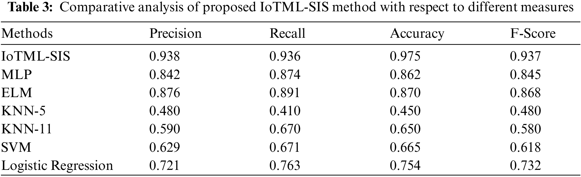
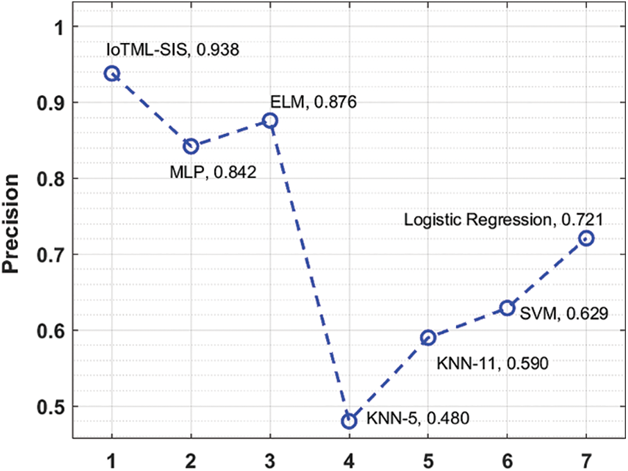
Figure 5: Precision analysis of IoTML-SIS model with existing techniques

Fig. 6 inspects the recall analysis of the IoTML-SIS manner with other existing methods. The figure note that the KNN-5 and KNN-11 approaches have offered lesser recall values of 0.410 and 0.670 correspondingly. Likewise, the SVM and LR manners have reached somewhat improved outcomes with the recall of 0.671 and 0.763. Also, the MLP and ELM algorithms have outperformed competitive outcomes with the recall of 0.874 and 0.891 correspondingly. But, the presented IoTML-SIS method has showcased the existing techniques with a maximal recall of 0.936.

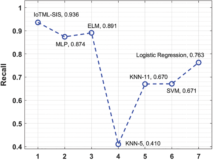
Figure 6: Recall analysis of IoTML-SIS model with existing techniques

Fig. 7 observes the accuracy analysis of the IoTML-SIS method with other recent algorithms. The figure specified that the KNN-5 and KNN-11 techniques have offered minimum accuracy values of 0.450 and 0.650 correspondingly. Similarly, the SVM and LR techniques have attained slightly increased results with the accuracy of 0.665 and 0.754. At the same time, the MLP and ELM manners have demonstrated competitive results with the accuracy of 0.862 and 0.870 correspondingly. Finally, the projected IoTML-SIS method has exhibited the existing approaches with a superior accuracy of 0.975.

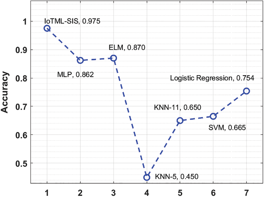
Figure 7: Accuracy analysis of IoTML-SIS model with existing techniques

Finally, Fig. 8 determines the F-score analysis of the IoTML-SIS manner with other existing approaches. The figure clear that the KNN-5 and KNN-11 methods have offered least F-score values of 0.480 and 0.580 respectively. Also, the SVM and LR techniques have achieved somewhat increased results with the F-score of 0.618 and 0.732. Besides, the MLP and ELM approaches have depicted competitive outcomes with the F-score of 0.845 and 0.868 correspondingly. Eventually, the presented IoTML-SIS methodology has demonstrated the recent methods with the higher F-score of 0.937.

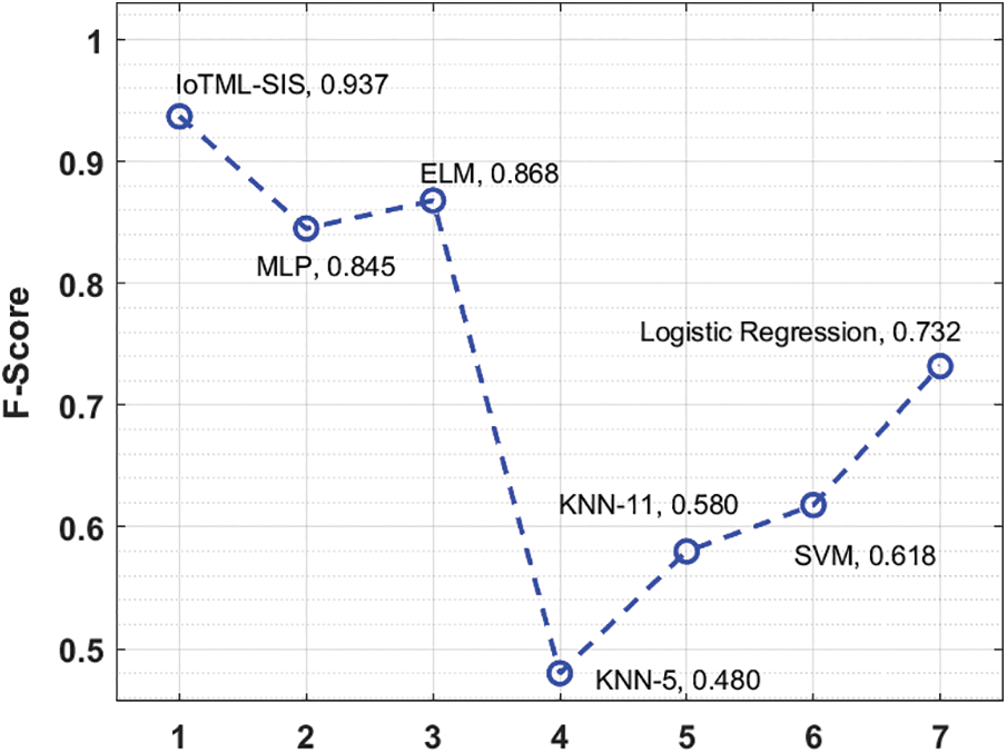
Figure 8: F-Score analysis of IoTML-SIS model with existing techniques

5  Conclusion

This paper has introduced a new IoTML-SIS for precision agriculture in order to effectively use the water resources in farmland. The proposed model involves three different processes namely data collection, LS-SVM based classification, and AAA based parameter tuning. During data collection phase, a set of sensors measure the farmland parameters and are fed into the ML model for classification purposes. The LS-SVM model is applied as a classifier to determine the required level of the water. Besides, the parameters involved in the LS-SVM model are tuned optimally using AAA to enhance the classification performance. The performance validation of the proposed IoTML-SIS technique ensured better performance over the compared methods interms of several evaluation parameters. The experimental results ensured that the IoTML-SIS technique is found to be an appropriate tool for smart irrigation in precision agriculture. In future, it can be deployed in real time environment.

Funding Statement: The authors extend their appreciation to the Deanship of Scientific Research at King Khalid University for funding this work under grant number (RGP 2/209/42). This research was funded by the Deanship of Scientific Research at Princess Nourah bint Abdulrahman University through the Fast-Track Research Funding Program.

Conflicts of Interest: The authors declare that they have no conflicts of interest to report regarding the present study.

This work is licensed under a Creative Commons Attribution 4.0 International License, which permits unrestricted use, distribution, and reproduction in any medium, provided the original work is properly cited.