DOI:10.32604/cmc.2022.023566
| Computers, Materials & Continua DOI:10.32604/cmc.2022.023566 | |
| Article |
A Novel Framework for Windows Malware Detection Using a Deep Learning Approach
Northern Border University, Arar, 9280, Saudi Arabia
*Corresponding Author: Abdulbasit A. Darem. Email: basit.darem@nbu.edu.sa
Received: 13 September 2021; Accepted: 20 December 2021
Abstract: Malicious software (malware) is one of the main cyber threats that organizations and Internet users are currently facing. Malware is a software code developed by cybercriminals for damage purposes, such as corrupting the system and data as well as stealing sensitive data. The damage caused by malware is substantially increasing every day. There is a need to detect malware efficiently and automatically and remove threats quickly from the systems. Although there are various approaches to tackle malware problems, their prevalence and stealthiness necessitate an effective method for the detection and prevention of malware attacks. The deep learning-based approach is recently gaining attention as a suitable method that effectively detects malware. In this paper, a novel approach based on deep learning for detecting malware proposed. Furthermore, the proposed approach deploys novel feature selection, feature co-relation, and feature representations to significantly reduce the feature space. The proposed approach has been evaluated using a Microsoft prediction dataset with samples of 21,736 malware composed of 9 malware families. It achieved 96.01% accuracy and outperformed the existing techniques of malware detection.
Keywords: Malware detection; malware analysis; deep learning; feature extraction; feature selection; cyber security
As cybercriminals continue to refine their tactics and adopt ingenious attack methods, cyberattacks are increasing drastically and have remained a serious issue to organizations and Internet users. The annual loss to world economy due to cybercrime is predicted to be more than $6 trillion by 2021 [1]. Moreover, cyberattacks are taking longer to resolve and cost organizations much more than before, with malware attacks being the most expensive costing businesses, about $2.6 million per attack [2]. Malware is any code that purposely executes malicious payloads on victim machines. It is a popular and prime attack vector as it is simple to deploy automatically and remotely. Malwares have been steadily evolving in terms of diversity, stealthiness and complexity over the past decades, making them undetectable by the conventional antimalware approaches. Kaspersky identified 24,610,126 unique malwares in 2019, which represents an increase of 14 percent over the previous year [3]. With the enormous profit that malware could yield to cybercriminals, cybercriminals have resorted to crafting malware that can cripple organization's entire network. The sustained evolution and diversity of malware make an efficient malware detection approach critical to protect organizations.
A wide variety of malware detection approaches have been developed over the years with increasingly deploying machine learning (ML) techniques. These malware detection studies have resulted in signature-based approach [4], behavioral approach [5], heuristic approach [6], and model-based approach [7]. These malware detection methods can be classified as static analysis based [8] or as dynamic analysis-based solutions [9]. In static analysis methods, malicious files are analyzed without executing them, whereas the files are required to execute in dynamic analyses methods. The execution of the malicious files must be done in a controlled (e.g., virtual machine or sandbox) environment. The static analysis can analyze malicious files fast provided that the files are not obscured or packed. In contrast, packing techniques do not affect much the dynamic analysis since the files are analyzed while they are being executed. However, newer malwares can detect the runtime environment (e.g., virtual environment) and may simply stop executing. Moreover, malware may only execute in certain circumstances [9] making the collection of malware behavior unattainable.
Malicious software (malware) detection is defined as the process of using some markers (e.g., features or signatures) to classify software code as either malware or benign. Malware is a software code developed by cyber criminals for nefarious purposes such as corrupting the system and data as well as stealing sensitive data. The malware caused damages are substantially increasing [10], thus, there is a need to detect malware efficiently and automatically and remove them quickly from the systems. Malware detection is an NP-complete problem [11] and thus it is a very challenging and difficult problem to solve. This challenge has sparked research to find effective solutions to the problem of malware detection. The conventional malware detection solutions are based on signatures extracted from malware by reverse engineering malware instances. These approaches are no longer effective as malware writers constantly modify malware signatures. The complexity of malware detection has also increased substantially with the increase of malware numbers at an alarming rate. Also, malware writers deploy various techniques to evade detection. While various new malware detection techniques have been developed using machine learning methods and deep learning [12–14], there are still improvements to be made in the accuracy of malware detection. Also, the performance of machine learning technique is affected by various factors including the parameters they use, the malware analysis process deployed, the type of features used. Therefore, the need to develop an efficient malware detection continue to be one of the major cyber security research quests.
In this paper, the problem of malware detection using a new sub area of machine learning methods commonly known as deep learning is addressed. Deep learning is evolving quickly and showing remarkable performance results in various application domains. It is also receiving increased attention in malware detection research [15]. The contribution can be summarized as follows:
• A novel approach based on deep learning for detecting malware called TRACE is proposed. Unlike the existing approaches that regard malware detection as a classification problem, the proposed approach deploys both regression as well as a classification technique and use various feature engineering techniques to significantly reduce the feature space.
• The proposed approach evaluated using Microsoft prediction dataset with samples of 21,736 malware composed of 9 malware families.
• The proposed approach achieved 96.01% accuracy, which is an improvement in the detection rate.
The rest of the paper is structured in the following manner. First the related work in malware detection is presented in Section 2. Section 3 presents the proposed malware detection method. Section 4 presents the complexity analysis. The performance evaluation is presented in Section 5. The results and discussion are highlighted in Section 6, followed by concluding remarks in Section 7.
Malware detection is an active research area within academic and commercial environments. An Wadkar et al. [12] proposed an approach for detecting malware evolution using SVM model. Abawajy et al. [13] proposed an ensemble-based approach referred to as a hybrid consensus pruning (HCP). HCP uses a consensus function to generate the base classifiers for the final ensemble. HCP is validated through AUC metric. Manavi et al. [16] developed an approach based on OpCode sequence and evolutionary algorithm. The OpCodes are extracted from the executables and a weighted graph is built. An evolutionary algorithm is used to build a graph for each malware family and benign code, which is used to compare with when performing classification. Li et al. [17] proposed a CNN-based malware detection approach. In the approach, virtual machine memory snapshot image of running malware and benign is captured and memory images converted to grayscale images, which is used for training and testing on the CNN-based model. Zhang et al. [18] present an approach for malware classification. The approach is based on data flow analysis to extract semantic structure features of the code and the graph convolutional networks (GCNs) for detection. The approach achieved 95.8% detection accuracy. In the approach proposed by Han et al. [19], malware is profiled based on its structure and behavior. It then uses several classifiers, namely Random Forest, Decision Tree, CNN, and XGBoost to classify the input data.
A method for malware detection based on visualization of the code texture was presented by Hassan et al. [15]. The approach deploys a version of Faster Region-Convolutional Neural Networks (RCNN) with transfer learning. The malicious code is mapped through visualization technology onto matching images with usual texture features to detect malware. The approach produced an accuracy of 92.8%. Huang et al. [20] developed a deep learning and visualization-based approach for detection of malware based on Windows API. It uses static features obtained from sample files to produce static visualization images. It then generates dynamic visualization images by using Cuckoo Sandbox to perform behavior analysis. Two images are then merged into hybrid images. Evaluation of a classification model based on static images and a classification model based on hybrid images were preformed showing that the latter performed better than the static approach alone. Marín et al. [21] proposed a malware detection and classification model based on network traffic. The model is based on deep learning and combines a convolutional neural network layer and the recurrent neural network layer in a different manner to create different models.

Approaches that exploit the generative adversarial network (GAN) have also been proposed in [10,24,27,28]. GAN uses a generator and a discriminator. The purpose of the discriminator to differentiate fake data from actual data. The purpose of the generator is to use a known probability distribution and generate fake data such that the discriminator will not be able to differentiate between the fake and actual data. An adaptive malware detection that mimics benign network traffic based on the GAN parameter is presented by Rigaki et al. in [27] . The approach proposed by Kim et al. [10] combines several deep learning approaches and uses the GAN components to generate fake malware from a given probability distribution and to learn the features of malware data. A detector is used in the approach learns different features of the malware from the actual and fake data. The proposed model achieves 95.74% average classification accuracy. A new adversarial attack that changes the bytes of the binary to create adversarial examples has also been proposed by Suciu et al. [28]. Tab. 1 summarizes some of the recent malware detection approaches based on machine learning techniques. Although a good effort is being expanded on solving the problem, it is obvious from the results that there is still some room for improvement. Also, exiting methods mainly approach the malware detection problem as a classification problem. In contrast, malware detection is viewed as a regression as well as a classification problem in the proposed work.
3 Proposed Malware Detection Approach
In this section, the proposed approach is discussed in detail. As shown in Fig. 1, the proposed framework has four different phases: (1) Data Pre-Processing phase; (2) Feature Processing phase; (3) Ensemble Classification phase, and (4) Malware Detection phase. Each of these phases is described in subsequent subsections.

Figure 1: The proposed malware detection framework with different phases and complete procedure of proposed framework
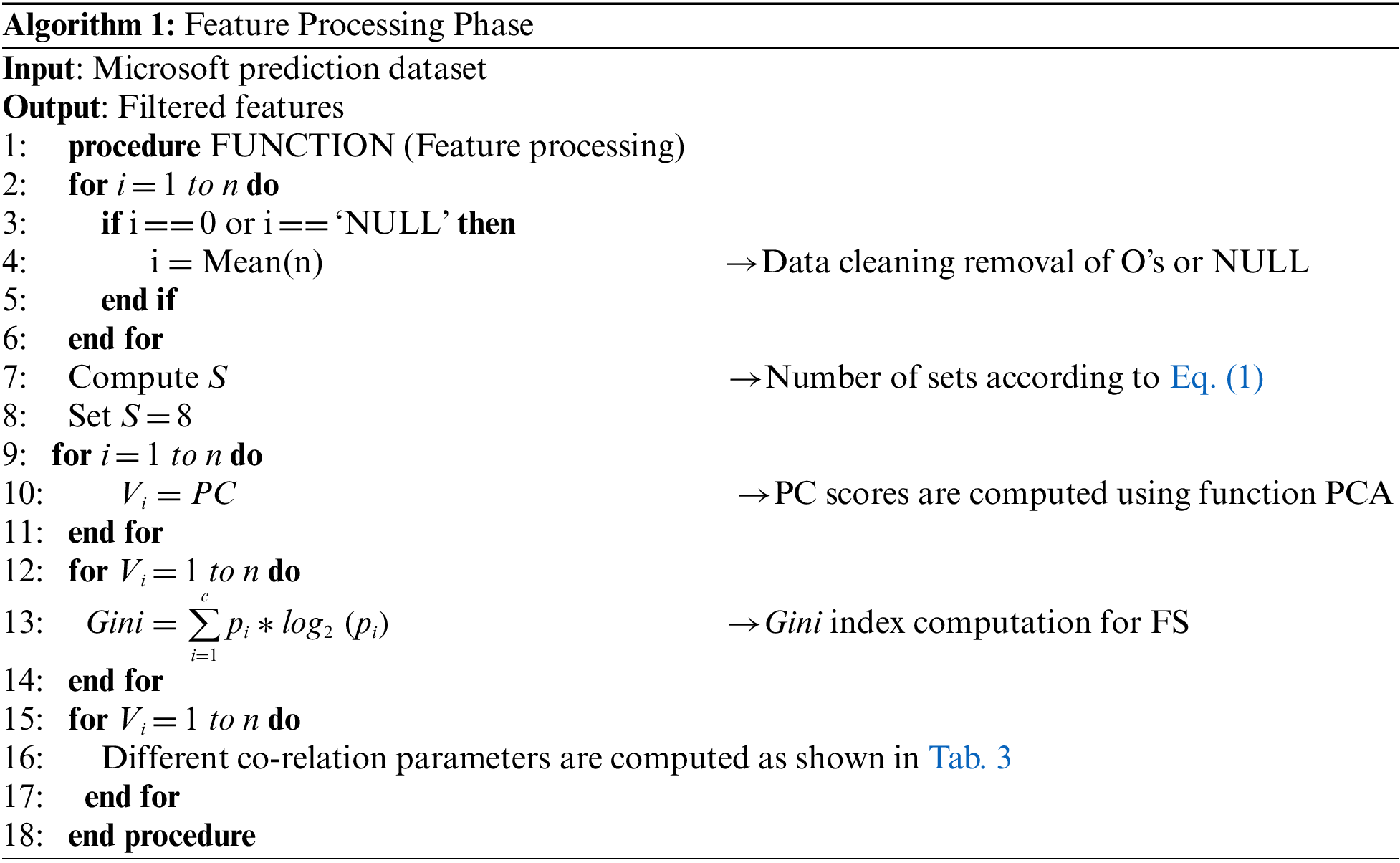
Algorithm 1 shows the process of generating a set of filtered features. The input to the algorithm is the raw Microsoft data set. The first set of steps (Line 1 to 6) perform basic data cleaning function followed by class balancing function (Line 7 to 8). The feature selection (Lines 12 to 14) and feature co-relations (lines 15 to 17) are performed. The output, which is a set of filtered features, is finally obtained. Each of these processes is described in the following subsections.
The preprocessing phase consists of two sub-phases namely data cleaning and class balancing. In this paper, the Microsoft prediction dataset with samples of 21,736 malware was used, where each malware in the dataset belongs to one of the 9 malware families (e.g., virus, worm and trojan). The dataset is full of not applicable (NAs) and NULL entries. Each cell of every feature should be noise-free and clean. To achieve this, the data set was cleaned by replacing the NA and the NULL values in the dataset with a mean value.
After cleaning, class balancing was performed. The data set's feature space explains its relevance as each feature has its own importance for contributing to the file. The features should be balanced with respect to the number of cases in each feature. The optimal ratio of multiple cases in each feature helps both in data balancing as well as in prediction. Since lower number of cases represents minor class and greater number of cases represents major class, it is essential to perform class balancing (i.e., balancing the minor and major classes). In this paper, SOTU (Split by Oversampling and Train by Under-fitting) technique was used for class balancing [29]. SOTU works by over-sampling the minor class with its multiple classes, where training is done in a single set at one time to avoid over-fitting. The set is created in such a manner that each set contains equal number of major class and minor class. For the formulation of sample sets, this Eq. (1) is followed.
where Ftrain denotes the training file, n is the number of samples features, xa and xb represent the instances of minor and major classes, respectively. In this work, the number of features is n = 83, and the generated sample sets are 8.
A clean and balanced data is passed on to this step. The feature processing phase consists of three steps: (1) feature reduction, feature selection and feature-co-relation.
This step is applied to reduce the dimensionality of the data. The Principal Component Analysis (PCA) was used for feature reduction. PCA is a multivariate process that converts the input data (i.e., a series of correlated variables) into an uncorrelated set of variables.
A principal component (PC) score is produced by multiplying each row with the uniform score of each column. The estimated component scores are the individual values that state the information regarding the variability of the data. Fig. 2 represents the first four PCs. The parameters computed using the PCA function are presented in Tab. 2.

Figure 2: Transformations of PCs

Feature selection is the process of identifying and selecting a subset of input variables that are most relevant to the target variable. A filter method based on random forest was used to rank the features. To rank the features, the method computes ‘Gini index’ score, which stands for data homogeneity. With the assistance of features, data is partitioned into the nodes. The value of the Gini is determined for both the root and the leaves. The mean value of Gini decrease is created after the analysis of the difference between the different Gini values. For the most critical function, this value is the highest. After selecting 41 features based on random forest, the features are further analyzed. This process is repeated until a feature is judged.
After selecting the 41 features, it is very important to find the relation among all the selected features. For this, we need to measure variance to determine how far observed values differ from the average of predicted values based on methods such as Root Mean Square Error (RMSE) (Eq. (2)), R2 score (Eq. (3), Mean Absolute Error (RAE) (Eq. (4)) and Mean Squared Error (RSE) (Eq. (5)). Tab. 3 shows the computed value of RMSE, R2 score, MAE, and RAE.

In the above equations,
To minimize bias and variance, ensemble learning (i.e., a collection of models) using four base classifiers: Light Gradient Boosting Machine (LightGBM), eXtreme Gradient Boosting (XGBoost), Convolutional Neural Network (CNN) and Long-Short Term Memory (LSTM) was deployed. LightGBM [30] is a gradient boosting platform which uses algorithms based on tree learning. It allows complete and effective use of the gradient boosting system by first processing the dataset and making it lighter. LightGBM is suitable for this study since it is able to process big datasets, runs fast and requires less memory. XGBoost [31], commonly used in machine learning technique, is also from a family of a gradient boosting. It is originated from Gradient Boosting Decision Tree (GBDT). It provides good accuracy and relatively fast speed compared to traditional machine learning algorithms. For performance, XGBoost chooses an algorithm based on histograms. The histogram-based algorithm uses bins that are separated by data point characteristics into discrete types. It is, therefore, more accurate than the pre-sorted process, but all the potential split points must be enumerated as well.
CNN [32] extracts the raw data directly and outputs the outcome of classification or regression in an end-to-end structure. CNN's neuron weights are trained via backpropagation algorithm. A collection of feature maps is generated by each convolution layer, while each feature map represents a high-level feature extracted through a specific convolution filter. The pooling layer primarily uses the local correlation theory to complete the down sampling, so features can be extracted from a more global perspective by the subsequent convolution layer. These substantially lower the weight parameters number as well as the estimation of a deep network's preparation. The LSTM [32], a commonly used deep neural network approach, is an enhanced Recurrent Neural Networks (RNNs) based model. RNN uses an internal state to represent previous input values, allowing temporal background to be captured. For long input sequence, it is not easy to train LSTM. However, compared to RNN, LSTM can capture the background of longer time series. In this problem, the census parameters are lengthy in nature, so to minimize the length, LSTM was used. This phase divided into two sub parts; firstly, opcode sequence and metadata feature of the low carnality features are extracted using de-compilation tools (i.e., CNN and LSTM). In the second part, the numerical features are extracted and trained by two different models, LightGBM and XGBoost. The features were treated separately because both feature sets reflect different patterns of information. Each classifier generates a normalized predicted score (NPS), NPS = S1, S2, …, Sn. The NPS indicates the likeliness of a given file to be malware infected or not and produced as illustrated in Algorithm 2.

Note that each classifier is an independent method and produces the classification decision as well as the class probability estimation. The estimator produced by all the classifiers are combined in Eq. (6). In this equation, hl is the classifier, which results in true prediction for k at a data point x.
This is the last phase of the TRACE framework where the decision is made about a given file. In this phase, the decision tree algorithm was deployed. This phase uses the normalized predicted score S1 to S4 generated in Algorithm 2 by each classifier. Based on this, the machine's reliability is derived using Eq. (7).
where d[i] is the rate of difference measured using the NPS vector and the real arrays. Using attribute importance score and error rate support, an NPS (i.e., S) is computed as follows:
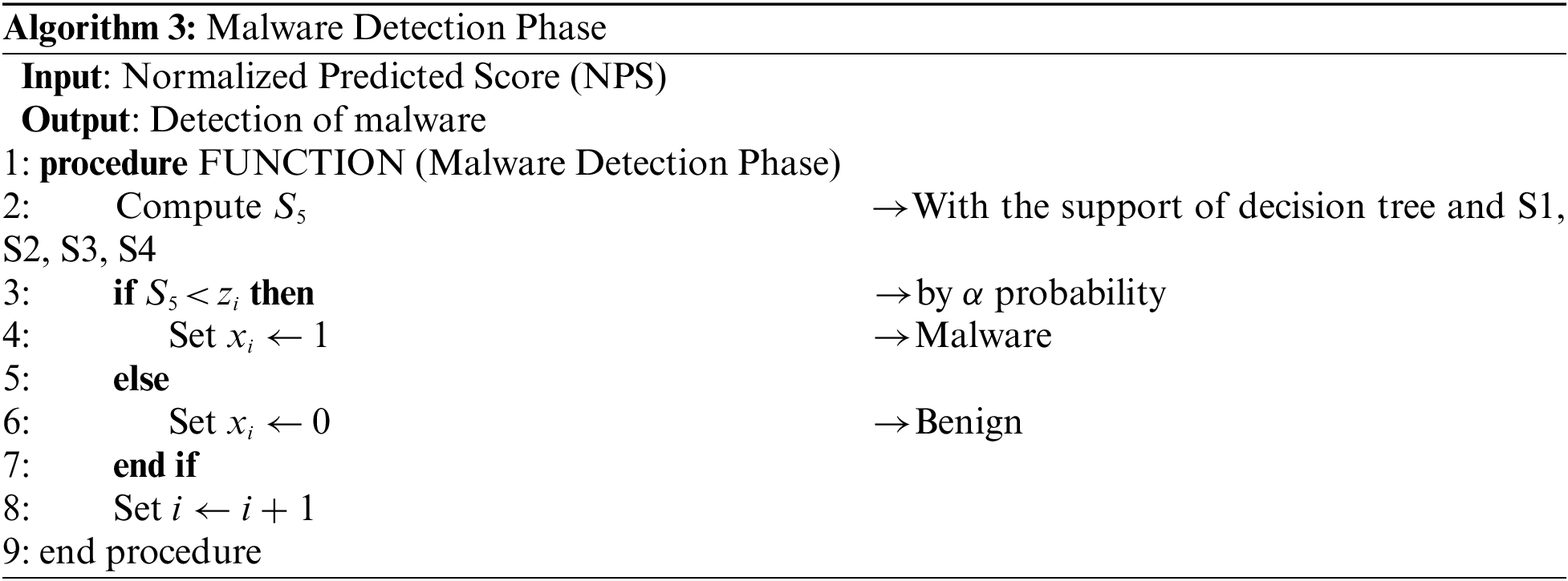
A threshold value is fixed by alpha probability to determine the decision. The complete procedure for the computation of the NPS and decision making is defined in the Algorithm 3. NPSs of all the models are used to train the decision tree.
It is essential to compute the complexity of the algorithm to ensure its validation. The Algorithms 1, 2, 3 illustrates each step followed in the proposed framework. Complexity is calculated by evaluating each step of the algorithm. Here, two different types of complexity are evaluated.
The number of iterations and the procedure of each iteration decide the time complexity. In Algorithm 1, steps 2 to 6 are comparison statements with n being the number of comparisons. Therefore, these steps take O(n) time. The loop in steps 9–11, the loop in 12–14, and steps 15–17 take O(n) time in the worst case. Therefore, the overall Algorithm 1 time complexity is O(n). In Algorithm 2, steps 2 and 3 perform assignments, thus they take O(1) time each. O(n) time is needed for steps 4–12 for the linear matrix formulation. The overall time complexity for Algorithm 2 is O(1) + O(n). Therefore, the worst time complexity is O(n) time. In Algorithm 3, the computation step like step 2 would take only O(1) time. The comparison steps 3 to 8 take O(n) time. In total, this algorithm requires O(n) time. The overall time complexity for all algorithms is
Therefore, the upper bound time complexity of the proposed algorithm is O(n).
The input data to each algorithm required n space. Each loop requires at most O(n) spaces whereas the arithmetic operations need O(1) space. The overall space complexity (SC) of the algorithm is given by:
Therefore, the upper bound space complexity of the proposed algorithm is O(n).
In this section, the performance evaluation of the proposed approach and compare the different algorithms (CNN, LSTM, LightGBM, XGBoost) was presented. In the first subsection, the experimental setup followed by the dataset used were discussed. Then, the impact and comparison of used approaches are discussed. Finally, the analysis of the proposed framework TRACE is discussed in the following subsection.
The CNN is designed with 64 layers: the input layers, convolution layers, fully connected layers, sequence layer, activation layer, pooling layers, combination layers, and output layers. The input to the CNN is 27 low cardinality features. The convolution layer is experimented to accept the input. At the activation layer, the ReLU activation function is considered with the same parameters as in convolution layer so that the accurate deep information is not lost. The key benefit of using the ReLU feature over other kernel function is that it does not simultaneously stimulate all the neurons. This implies that the neurons are only deactivated if the linear transformation output is less than 0. The effect of negative input values is zero, which means that the neuron is not triggered. As only a certain number of hidden neurons are activated, when contrasted to the sigmoid or tanh function, the ReLU function is much more computationally effective. Sigmoid activation function was used at the last layer as only spamicity score is expected from the model. Maximum pooling method is adopted as pooling layer. The parameters for the same are 28*28*32, keeping the filter size also the same. The highest proportion is taken and placed in a new grid for each filtered element. This is simply taking the most significant features and compressing them into one vector.
The LSTM network starts with two key layers, namely an input sequence layer and an LSTM layer. In sequence or time series, a sequence input layer enters information into the network. The LSTM layer is used to learn the long-lasting dependency among the time periods of the sequence information. For class labels predictions, the LSTM network will have a fully connected layer, a SoftMax layer, and an output classification layer. The sources size was set to be 41 sequences (the size of the input data). The network architecture consists of bidirectional LSTM layer of 100 concealed units and yields the last part of the series. The final network has 41 classes by including a completely connected layer of size 9 followed by a layer of softmax and a classification layer. For training the device using LSTN, data is loaded in the same manner as in CNN. For padding, the LSTM network partitions the training sample dataset into dinky-batches. To ensure that the segments have the same length, the network applies padding. For training and testing, the train Network use feature is used to train the LSTM network. The testing is done in the same way as the training, except for the data being the difference. The NPS rating is generated following testing.
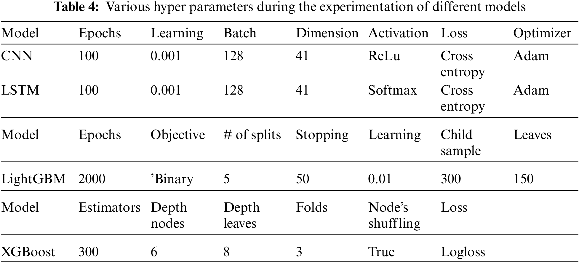
Windows 64bit operating system was used with the support of 8GB RAM. Also, Python programming language was used with Python libraries, for example, TensorFlow, Docker Server, Anaconda. The hyper-parameters considered in all the models are shown in Tab. 4.
To perform the experiments, publicly available Microsoft Malware Prediction dataset was used. This data set is created for Research Prediction Competition at Kaggle [33]. This dataset contains 83 features in total and contains noise and imbalanced data. The dataset consists of three files, i.e., sample submission, test, and train. The proposed scheme focused on balancing the data and making the data ready for experiments. Around 21,736 malwares were used that come from 9 different malware families.
As a performance metric to validate the efficiency of proposed framework TRACE, the following parameters were used to compare the results of all the deep learning algorithms. In the equations, the term TP denotes the true positive, FP is the false positive, TN denotes the true negative, and FN denotes the false negative. The accuracy metric (Eq. (11)) quantifies the ratio of correctly judged results by the model.
Also AUC (Area Under the Curve) was used to determine which of the used models predicts the classes best. AUC is based on the false positive rate (FPR) and the true positive rate (TPR). The true positive rate, also known as recall, quantifies the number of valid classifications made by the classifier out of all observations that are true.
The false positive rate (FPR) measures the ratio of false positives within the negative samples and computed as follows:
The Precision quantifies the number of positive class predictions that belong to the positive class and computed as follows:
F1 score (Eq. (15) is defined as weighted average of recall (Eq. (12)) and precision (Eq. (14)), thus balances any concerns associated with the recall and precision results.
where β reflects recall vs. precision.
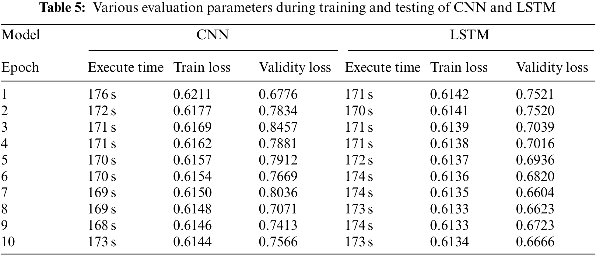
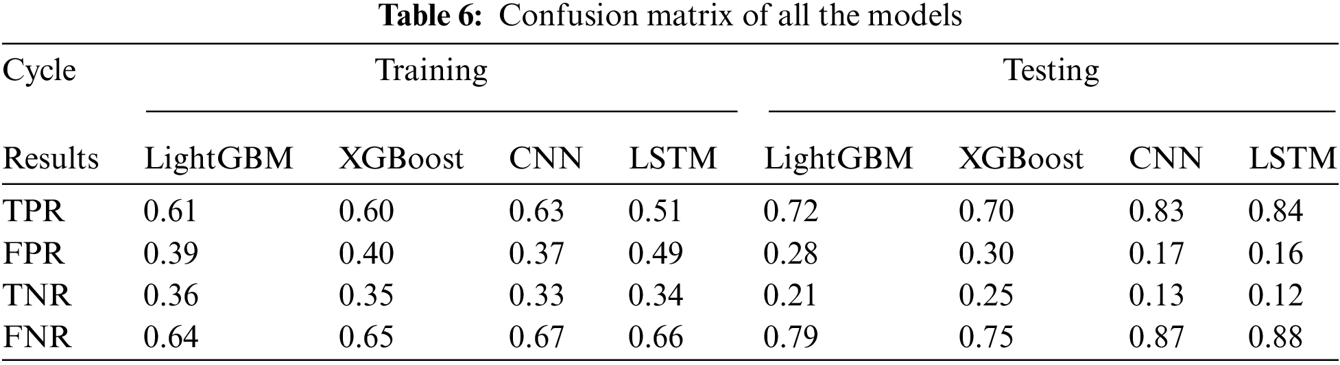
It is important to look at the performance of the deep learning models when working with a large dataset like the Microsoft Malware Prediction Competition dataset. As noted early, the dataset was transformed into a sparse matrix (SM) so that it can be used by the deep learning models as well as the decision tree model. The SM with an LGBM baseline model were paired in this experiment. For memory management purposes, the information was partitioned into smaller chunks of 120000 rows (sample set produced by SOTU). Tab. 5 shows some of the performance data for LSTM and CNN. The confusion matrix was used to measure the performance of the LSTM, LightGBM, XGBoost and CNN models. The results of all the models are shown in Tab. 6 in terms of (TPR), (FPR), true negative rate (TNR) and false negative rate (FNR). In terms of TPR, LSTM performs better than the other models.
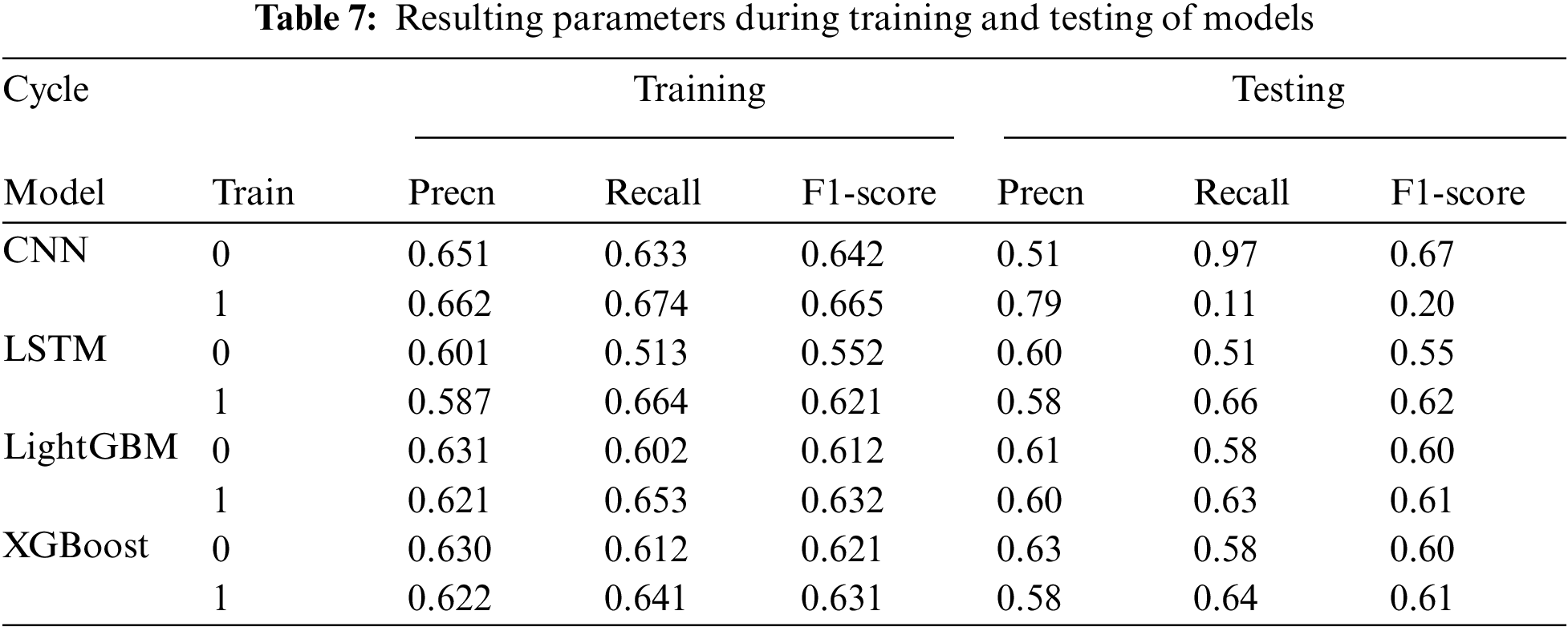
Tab. 7 shows the performance of LSTM, LightGBM, XGBoost and CNN models in terms of precision, recall and F1-score computed during the training and testing of the models. To evaluate the efficiency and effectiveness of the proposed framework TRACE, a discrimination probability which is computed in the last phase of the framework was used. This probability is computed by combining the results of all the four models (CNN, LSTM, LightGBM, XGBoost), i.e., S1, S2, S3, and S4. This probability indicates the likelihood of malware injected into the machine. Our framework TRACE took 220 s, and the estimation of malware significantly outperformed the other methods.
Next, results were presented when TRACE is compared against other models with respect to True Positive Rate (TPR) (Fig. 4), F-score (Fig. 3), and AUC (Area Under Curve) (Fig. 5). Fig. 3 shows the malware detection performance of TRACE (i.e., Decision) as compared to others in terms of F-score metrics. From the diagram, it can be observed that TRACE (i.e., Decision in the graph) outperforms the other approaches substantially. This is because all the other models significantly contributed to the results of malware detection of TRACE model. Fig. 4 shows the malware detection performance of TRACE (i.e., Decision) with respect to TPR as compared to other models. TRACE (i.e., Decision in the graph) performs best in terms of TPR as it efficiently combines the results of other models. Fig. 5 shows the malware detection performance of TRACE (i.e., Decision) with respect to AUC as compared to other models. TRACE (i.e., Decision in the graph) performs best in terms of AUC as it efficiently combines the results of other models. From this graph, it can be observed that TRACE (i.e., Decision) achieves a precision of 96.01% whereas LSTM and CNN achieve slightly under 80%, and LightGBM and XGBoost achieve about 80%.

Figure 3: Malware detection performance of TRACE (i.e., decision) with respect to F-score

Figure 4: Malware detection performance of TRACE (i.e., decision) with respect to TPR

Figure 5: Malware detection performance of TRACE (i.e., decision) with respect to AUC
Malware is at the root of many cyber-security threats, including national security threats. It is estimated that cyber-attacks are the most dangerous security issue in the world today. Sometimes a single cyber-security breach may cost more than the cost of many natural disasters. The race between cyber-attackers and anti-malware tool developers is never ending. Therefore, researchers must put sustained pressure on cyber criminals to ensure that malware is detected as early as possible. To this end, a malware detection algorithm called TRACE was proposed, which combines malware analysis, feature extraction and deep learning architectures. Unlike the existing approaches that regard malware detection as a classification problem, the proposed approach deploys both regression as well as a classification technique and use various feature engineering techniques to significantly reduce the feature space. Extensive performance evaluation indicates that the proposed mechanism maintains outstanding classification capability. The proposed method achieved 96.01% precision, outperforming other models. In addition, the efficiency of the proposed model was measured to validate the efficacy and sustainability of various deep learning approaches. On average, it only took 0.76 s for TRACE to identify a fresh file.
Acknowledgement: The author extends his appreciation to the Deputyship for Research and Innovation, Ministry of Education in Saudi Arabia for funding this research work through project number 1385. The help of Prof. Jemal Abawajy is greatly appreciated.
Funding Statement: This research was funded by the Deputyship for Research and Innovation, Ministry of Education in Saudi Arabia through Project Number 1385.
Conflicts of Interest: The author declares that he has no conflicts of interest to report regarding the present study.
1. P. CISCO Report, “Cybersecurity Almanac:100 Facts, Figures and Statistics, “Report by cisco,” https://cybersecurityventures.com/cybersecurity-almanac-2019/, 2019 (accessed October 2020). [Google Scholar]
2. N. A. C. Accenture, “The cost of Cybercrime Study Report by accenture,” https://www.accenture.com/acnmedia/pdf-96/accenture-2019-cost-of-cybercrime-study-final.pdf, 2019 (accessed MARCH 6, 2020). [Google Scholar]
3. K. Kaspersky, “Malware Report by kaspersky,” https://go.kaspersky.com/rs/802-IJN-240/images/KSB2019StatisticsEN.pdf, 2019 (accessed October 2020). [Google Scholar]
4. H. Sun, X. Wang, R. Buyya and J. Su, “Cloudeyes: Cloud-based malware detection with reversible sketch for resource-constrained internet of things (iot) devices,” Software: Practice and Experience, vol. 47, no. 3, pp. 421–441, 2017. [Google Scholar]
5. H. S. Galal, Y. B. Mahdy and M. A. Atiea, “Behavior-based features model for malware detection,” Journal of Computer Virology and Hacking Techniques, vol. 12, no. 2, pp. 59–67, 2016. [Google Scholar]
6. A. V. Kozachok and V. I. Kozachok, “Construction and evaluation of the new heuristic malware detection mechanism based on executable files static analysis,” Journal of Computer Virology and Hacking Techniques, vol. 14, no. 3, pp. 225–231, 2018. [Google Scholar]
7. T. Lu and S. Hou, “A two-layered malware detection model based on permission for android,” in 2018 IEEE Int. Conf. on Computer and Communication Engineering Technology (CCET), IEEE, Beijing, China, pp. 239–243, 2018. [Google Scholar]
8. J. H. Abawajy and A. Kelarev, “Iterative classifier fusion system for the detection of android malware,” IEEE Transactions on Big Data, vol. 5, no. 3, pp. 282–292, 2019. [Google Scholar]
9. J. Jeon, J. H. Park and Y. -S. Jeong, “Dynamic analysis for iot malware detection with convolution neural network model,” IEEE Access, vol. 8, pp. 96899–96911, 2020. [Google Scholar]
10. J. -Y. Kim, S. -J. Bu and S. -B. Cho, “Zero-day malware detection using transferred generative adversarial networks based on deep autoencoders,” Information Sciences, vol. 460, pp. 83–102, 2018. [Google Scholar]
11. O. A. Aslan and R. Samet, “A comprehensive review on malware detection approaches,” IEEE Access, vol. 8, pp. 6249–6271, 2020. [Google Scholar]
12. M. Wadkar, F. Di Troia and M. Stamp, “Detecting malware evolution using support vector machines,” Expert Systems with Applications,” vol. 143, pp. 113022, 2020. [Google Scholar]
13. J. H. Abawajy, M. Chowdhury and A. Kelarev, “Hybrid consensus pruning of ensemble classifiers for big data malware detection,” IEEE Transactions on Cloud Computing, vol. 8, no. 2, pp. 398–407, 2020. [Google Scholar]
14. Y. Zhao, W. Cui, S. Geng, B. Bo, Y. Feng et al., “A malware detection method of code texture visualization based on an improved faster rcnn combining transfer learning,” IEEE Access, vol. 8, pp. 166 630–166 641, 2020. [Google Scholar]
15. M. Hassan, S. Huda, S. Sharmeen, J. Abawajy and G. Fortino, “An adaptive trust boundary protection for iiot networks using deep-learning feature extraction based semi-supervised model,” IEEE Transactions on Industrial Informatics, 17(4), pp. 2860–2870, 2020. [Google Scholar]
16. F. Manavi and A. Hamzeh, “A new approach for malware detection based on evolutionary algorithm,” in GECCO ‘19: Proc. of the Genetic and Evolutionary Computation Conf., New York, NY, USA, Association for Computing Machinery, 2019. [Online]. Available: https://doi-org.ezproxy-b.deakin.edu.au/10.1145/3319619.3326811. [Google Scholar]
17. H. Li, D. Zhan, T. Liu and L. Ye, “Using deep-learning-based memory analysis for malware detection in cloud,” in 2019 IEEE 16th Int. Conf. on Mobile Ad Hoc and Sensor Systems Workshops (MASSW), Monterey, CA, USA, pp. 1–6, 2019. [Google Scholar]
18. Y. Zhang and B. Li, “Malicious code detection based on code semantic features,” IEEE Access, vol. 8, pp. 176 728–176 737, 2020. [Google Scholar]
19. W. Han, J. Xue, Y. Wang, Z. Liu and Z. Kong, “Malinsight: A systematic profiling-based malware detection framework,” Journal of Network and Computer Applications, vol. 125, pp. 236–250, 2019. [Google Scholar]
20. X. Huang, L. Ma, W. Yang and Y. Zhong, “A method for windows malware detection based on deep learning,” Journal of Signal Processing Systems, 93.2, pp. 265–273, 2020. [Google Scholar]
21. G. Marín, P. Caasas and G. Capdehourat, “DeepMAL-deep learning models for malware traffic detection and classification,” in Data science–analytics and applications, Wiesbaden: Springer Fachmedien Wiesbaden, pp. 105–112, 2021. [Google Scholar]
22. Al-Dujaili, A. Huang, E. Hemberg and U. -M. O'Reilly, “Adversarial deep learning for robust detection of binary encoded malware,” in 2018 IEEE Security and Privacy Workshops (SPW), IEEE, San Francisco, CA, USA, pp. 76–82, 2018. [Google Scholar]
23. K. Grosse, N. Papernot, P. Manoharan, M. Backes and P. McDaniel, “Adversarial examples for malware detection,” in European Symp. on Research in Computer Security, Oslo, Norway, Springer, pp. 62–79, 2017. [Google Scholar]
24. J. -Y. Kim, S. -J. Bu and S. -B. Cho, “Malware detection using deep transferred generative adversarial networks,” in Int. Conf. on Neural Information Processing, Guangzhou, China, Springer, pp. 556–564, 2017. [Google Scholar]
25. W. Hu and Y. Tan, “Generating adversarial malware examples for black-box attacks based on gan,” arXiv preprint arXiv: 1702.05983, 2017. [Google Scholar]
26. Q. Wang, W. Guo, K. Zhang, A. G. Ororbia, X. Xing et al.., “Adversary resistant deep neural networks with an application to malware detection,” in Proc. of the 23rd ACM SIGKDD Int. Conf. on Knowledge Discovery and Data Mining, Nova Scotia, Canada, pp. 1145–1153, 2017. [Google Scholar]
27. M. Rigaki and S. Garcia, “Bringing a gan to a knife-fight: Adapting malware communication to avoid detection,” in 2018 IEEE Security and Privacy Workshops (SPW), IEEE, San Francisco, CA, USA, pp. 70–75, 2018. [Google Scholar]
28. O. Suciu, S. E. Coull and J. Johns, “Exploring adversarial examples in malware detection,” in 2019 IEEE Security and Privacy Workshops (SPW), IEEE, San Francisco, CA, USA, pp. 8–14, 2019. [Google Scholar]
29. A. Makkar and N. Kumar, “Cognitive spammer: A framework for pagerank analysis with split by over-sampling and train by under-fitting,” Future Generation Computer Systems, vol. 90, pp. 381–404, 2019. [Google Scholar]
30. M. Al-kasassbeh, M. A. Abbadi and A. M. Al-Bustanji, “Lightgbm algorithm for malware detection,” in Science and Information Conf., Springer, London, United Kingdom, pp. 391–403, 2020. [Google Scholar]
31. W. Niu, X. Zhang, X. Du, T. Hu, X. Xie et al., “Detecting malware on x86-based iot devices in autonomous driving,” IEEE Wireless Communications, vol. 26, no. 4, pp. 80–87, 2019. [Google Scholar]
32. B. Athiwaratkun and J. W. Stokes, “Malware classification with lstm and gru language models and a character-level cnn,” in 2017 IEEE Int. Conf. on Acoustics, Speech and Signal Processing (ICASSP), IEEE, New Orleans, LA, USA, pp. 2482–2486, 2017. [Google Scholar]
33. Microsoft, “Microsoft malware prediction,” https://www.kaggle.com/c/microsoft-malware-prediction/overview, 2018 (accessed September 18, 2020). [Google Scholar]
 | This work is licensed under a Creative Commons Attribution 4.0 International License, which permits unrestricted use, distribution, and reproduction in any medium, provided the original work is properly cited. |