Computers, Materials & Continua DOI:10.32604/cmc.2022.024109
Article

Hybrid Deep Learning Enabled Air Pollution Monitoring in ITS Environment

Ashit Kumar Dutta1, Jenyfal Sampson2, Sultan Ahmad3, T. Avudaiappan4, Kanagaraj Narayanasamy5,*, Irina V. Pustokhina6 and Denis A. Pustokhin7

1Department of Computer Science and Information Systems, College of Applied Sciences, AlMaarefa University, Ad Diriyah, Riyadh, 13713, Kingdom of Saudi Arabia
2Department of Electronics and Communication Engineering, Kalasalingam Academy of Research and Education, Krishnankoil, 626128, India
3Department of Computer Science, College of Computer Engineering and Sciences, Prince Sattam Bin Abdulaziz University, Al-Kharj 11942, Saudi Arabia
4Department of Computer Science and Engineering, K. Ramakrishnan College of Technology, Tiruchirappalli, 621112, India
5Department of Computer Applications, J. J College of Arts and Science (Autonomous), Affiliated to Bharathidasan University, Pudukkottai, 622422, India
6Department of Entrepreneurship and Logistics, Plekhanov Russian University of Economics, 117997, Moscow, Russia
7Department of Logistics, State University of Management, 109542, Moscow, Russia
*Corresponding Author: Kanagaraj Narayanasamy. Email: kanagaraj.n.in@ieee.org
Received: 05 October 2021; Accepted: 09 December 2021

Abstract: Intelligent Transportation Systems (ITS) have become a vital part in improving human lives and modern economy. It aims at enhancing road safety and environmental quality. There is a tremendous increase observed in the number of vehicles in recent years, owing to increasing population. Each vehicle has its own individual emission rate; however, the issue arises when the emission rate crosses a standard value. Owing to the technological advances made in Artificial Intelligence (AI) techniques, it is easy to leverage it to develop prediction approaches so as to monitor and control air pollution. The current research paper presents Oppositional Shark Shell Optimization with Hybrid Deep Learning Model for Air Pollution Monitoring (OSSO-HDLAPM) in ITS environment. The proposed OSSO-HDLAPM technique includes a set of sensors embedded in vehicles to measure the level of pollutants. In addition, hybridized Convolution Neural Network with Long Short-Term Memory (HCNN-LSTM) model is used to predict pollutant level based on the data attained earlier by the sensors. In HCNN-LSTM model, the hyperparameters are selected and optimized using OSSO algorithm. In order to validate the performance of the proposed OSSO-HDLAPM technique, a series of experiments was conducted and the obtained results showcase the superior performance of OSSO-HDLAPM technique under different evaluation parameters.

Keywords: Deep learning; air pollution; environment monitoring; internet of things; intelligent transportation systems; oppositional learning; LSTM model

1  Introduction

The advancements made in technology and economic growth have resulted in increasing demands for Intelligent Transportation System (ITS) for traffic service system. The need towards the development of real time data system about ITS is prominently increasing [1]. Real-time traffic data like traffic flow, travel time, traffic congestion, and average vehicle speed can be utilized by different stakeholders such as ministry of transportation, common users and other government bodies to enhance the roadway service levels. Various methods have been introduced for collecting and sending real time traffic data to traffic data centers through several networks. The rise in vehicles on road and the resultant traffic are characteristics of the modern world and this phenomenon implies that a number of interrelated problems such as long travel times, pollution (noise and air), traffic accidents, and so on, are growing in a similar manner. Various reports have been published so far to determine the range of problems faced during traffic and it led to the growth of a novel field of studies to be specific [2]. ITS has become an essential component in enhancing both modern economy and human life. It is aimed at improving the road traffic by understanding the capability of roads, reducing energy consumption, improving the quality of environments and driver safety amongst several things. Furthermore, growth is anticipated in the domain of ITS in which ideas like big data can be incorporated. Thus, it led to a modern conception of ‘Internet of Vehicles’ (IoV).

A vehicle's performance parameters like mileage, speed, air pressure, mechanism, and condition of tires are monitored by Internet of Things (IoT) interface scheme. Likewise, engine oil and vehicle pollution conditions are also monitored with the help of IoT. This automated monitoring system is extremely helpful in alerting and saving a driver's life from accident. The primary reason for vehicle pollution is inappropriate maintenance and untimely monitoring of the vehicles. Therefore, automated scheme is required to monitor and maintain the vehicles which in turn control and reduce the pollution. IoT-based method plays a smart role in this domain and monitors the vehicle conditions in terms of pollution and vehicle controls from time-to-time. It can simply detect the tire pressure, speed, engine performance, and fuel level. Smart Vehicle Monitoring Scheme (SVMS) has been presented earlier on the basis of IoT system. This SVMS scheme is utilized for the prevention of theft and accidents for the vehicle. Further, this scheme is also employed for accessing and controlling vehicles with safety conditions. IoT system is utilized for marinating and controlling the traffic, vehicle tracing and time, and driver management. Intelligent Transport System (ITM) is used to understand about the climate and road conditions. Vehicles tracking scheme, Global Positioning System (GPS), and accident safety precautions have been deliberated to safeguard the life of passengers and the driver. Innovative global navigation satellite systems and driver assistance system-based IoT concepts have been proposed earlier. IoT system further monitor the liquor level of the driver and vehicle speed using controllers. IoT-intelligent transport and smart vehicle technology systems have been proposed earlier using various methods [3].

In literature, IoV technique has been presented in electrical automatic vehicles. Both network and controller are significant factors in automatic vehicles [4]. IoV concepts have been presented in communication technology and intelligent transportation systems [5]. Global Positioning System (GPS) is utilized for estimating the location and speed of the vehicle. Cloud database management scheme is employed for information analysis and storage so as to monitor the performance of the engine [6]. Air pollution levels are under check in these IoT-based systems. Pollution monitoring has been improved by distinct sensor nodes and wireless sensor networks. The information associated with pollution is analyzed and stored using cloud computing technique. IoT system monitors the pollution level of the vehicle and take corrective measures to decrease the levels of pollution. In literature, IoT applications have been widely investigated and applied in distinct facets of society while researchers are actively engaged in development of this futuristic concept [7].

In this background, the current paper presents a technique named Oppositional Shark Shell Optimization with Hybrid Deep Learning Model for Air Pollution Monitoring (OSSO-HDLAPM) for ITS environment. The proposed OSSO-HDLAPM technique deploys an array of sensors in vehicles to measure pollutant level. The data is then transmitted to cloud environment for further processing. In addition, a hybridized Convolution Neural Network with Long Short-Term Memory (HCNN-LSTM) model is used to predict the level of pollutants based on the data attained earlier by the sensors. In HCNN-LSTM model, the hyperparameters are selected and optimized using OSSO algorithm. In order to validate the efficacy of the proposed OSSO-HDLAPM technique, a sequence of experimentations was conducted and the results were examined under dissimilar aspects.

2  Literature Review

This section reviews the recent state-of-the-art air pollution monitoring techniques developed for ITS environment. Dweik et al. [8] designed the structure of a modular, Scalable Enhanced Road Side Unit to utilize it as part of a wide ITS depending on IoT model. The presented unit is planned for data collection utilizing a change in sensors and on-board camera. The gathered data is then uploaded in the central server to act according to the situation, for instance speed limit alteration, metering routes to reduce vehicle congestion and emission, and problems in weather advisory warnings. Kaivonen et al. [9] defined the utilization of wireless sensors on Uppsala buses and used a combination of mobile sensor networks with GreenIoT testbed. An extensive investigation was conducted to evaluate the communication as well as data qualities of the proposed model.

Ogundoyin [10] presented a secure, autonomous, anonymous, and privacy-preserving traffic undertaking analysis method for ITS. In the presented method, fine-grained traffic data like average speed are attained in the absence of privacy of the cooperating users’. The model utilized both altered Paillier cryptosystem and Chinese Remainder Theorem for aggregating heterogeneous road data to save bandwidth and Boneh short signature for authentication. The presented technique has been autonomous and permitted the user to generate their own private or public key pair for communication. Shen et al. [11] suggested an optimum parking site selection method to get rid of CO2 emission from traffic flow in green urban road network. Inspired from dynamic traffic zone programming, the constrained optimized technique is set up for assessing the influence of potential Public Parking Location (PPL) on road traffic emission. During all the conditions, Thiessen Polygon-based zoning technique was applied to investigate road traffic distribution. The vital involvement of this analysis is that the presented technique primarily considers CO2 emissions of the entire traffic network of maintainable city progress as the optimized purpose instead of considering only the usually discussed travel distance or cost effectiveness. Secondly, a Thiessen polygon-based public parking zoning technique was established and executed realistically. Thirdly, GA was utilized to find the optimum PPL set. GA is a huge application value from speeding up stochastic search to global optimization.

In the study conducted earlier [12], a method was developed to estimate and classify the traffic congestion state of distinct road segments in a city by examining road traffic data collected from in-road stationary sensors. ANN-based scheme was utilized in the classification of traffic congestion states. According to traffic congestion status, ITS automatically upgrades the traffic regulations such as varying the queue length from traffic signals, signifying alternate routes etc., In [13], a dynamic route planning technique in urban conditions was presented to distribute traffic density from immediate to another minimum dense traffic junction. The presented structure attempts at minimizing the amount of congested traffic junctions by uniformly distributing the immediate traffic, with the help of diversion suggestion. This way, dense air pollution gets decreased at traffic junctions. The presented structure relies on IoT framework to process the geographic data immediately, to reduce the quantity of air pollution and time of exposure to the commuter who passes by the junction.

In order to generate and utilize the immediate data as well as historical record [14], both data-driven manners with model-driven manners are required. Primarily, the restrictions of two baseline manners such as auto-regressive combined affecting average and periodical affecting average technique are explained. Second, ANN is implemented in hybrid forecasting technique to balance between the techniques. The trained NN allows the ANN for weighting amongst immediate traffic information and traffic pattern exposed by historical traffic data. Moreover, an emergency manner, utilizing the Bayesian network, has also been used to the forecasted method to handle traffic accidents or emergency conditions.

3  The Proposed Model

The presented model is compact and lightweight on automobiles. It is certain that the model will assist in the reduction of harmful gases from the vehicle. The architecture of the proposed model is shown in Fig. 1. The authors assure that the proposed model is set to bring a dramatic change in control and prevention measures for air pollution. Both sensor and the other element utilized in the construction of the scheme are significantly less expensive and therefore, the scheme is cost-efficient. The sensor is applied in the detection of pollutants, discharged by vehicles, such as carbon monoxide (CO), Ozone, Sulphur dioxide (SO2), nitrogen dioxide (NO2), and Particulate Matter (PM2.5). In literature, various kinds of sensors such as MQ135, MQ7, and MQ2 are employed to gather distinct kinds of emission information [15]. MQ7 is highly sensitive to carbon monoxide. MQ2 is associated with the detection of gas leakages. MQ135 is utilized in the detection of NOx, NH3, benzene, alcohol, CO2, smoke, and so on.

The values gathered by every sensor are collected at Arduino board. Arduino is programmed in such a manner that it collects data from distinct sensor nodes and compares it with average values. The values collected at the Arduino board are stored in a dataset. It assists in monitoring the changes that occur in air at distinct time periods. When there is a sufficient value present in the database, the data collected can be utilized for creating a method that could make predictions and analyses. The method employs a machine learning approach i.e., decision forest regression algorithm, to learn about the distinct values that may exist in the database. After learning process gets completed, the method is currently prepared to draw inference on distinct pollutants present in the air and predict the pollutants’ level in future.

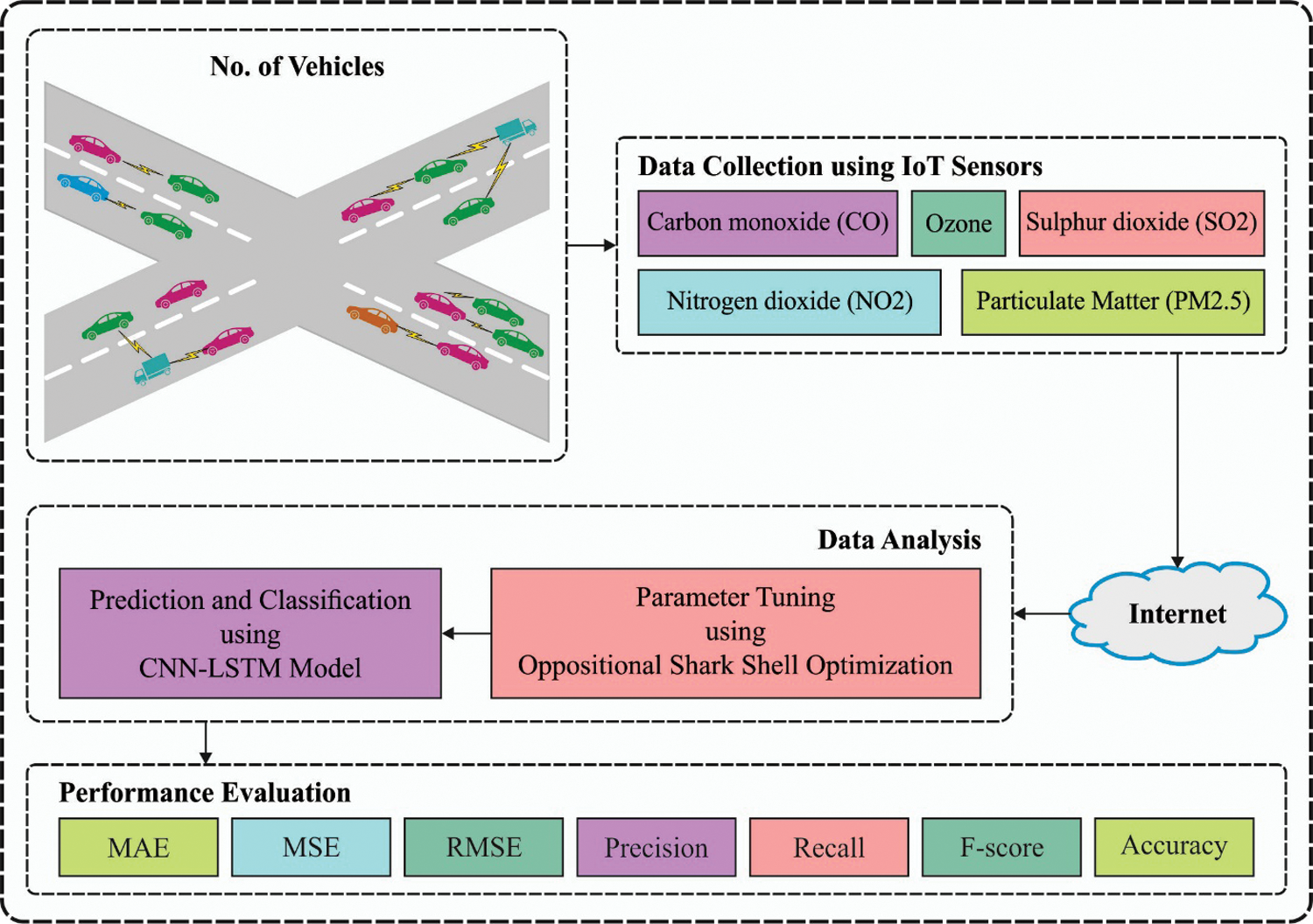
Figure 1: System architecture of OSSO-HDLAPM technique

3.1 Process Involved in HCNN-LSTM Based Predictive Model

In HCNN-LSTM model, the merits of both CNN and LSTM models are integrated. Two CNN layers are utilized to assure the association and to extract the multi-dimensional data efficiently. The basic structure of CNN is given in Fig. 2. The features from CNN layer can be applied to LSTM model. Time-dependency is additionally derived in LSTM layer. A set of three Fully Connected (FC) layers are present in the model such as FC1, FC2, and FC3. Two initial FC layers are used to attain the features derived via CNN layer whereas the last FC layer is applied to perform prediction process [16]. The input and output data in CNN layer are represented as given in Eq. (1):

train_xi[x11x12⋯x1qx21x22⋯x2q⋯⋯⋯⋯xp1xp2⋯xpq],train−yi=[vart−p+3,vart−p+4,…,vart+1,vart+2,…,vart+q,]T,(1)

where p and q denote the step size and data feature respectively. The ith instance from training data is passed onto the model. At initial convolutional layer (1stConV), the number, convolutional kernel size, and step length are represented by ter−size=(m,n),filter−num, and strides, correspondingly.

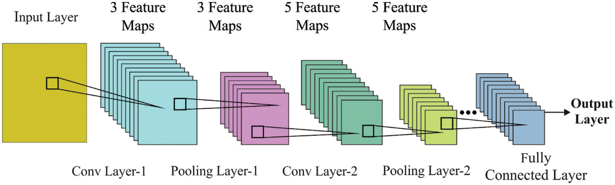
Figure 2: Overview of CNN model

The jth convolutional kernel Wj can be defined as follows.

Wj=[w11w12⋯w1nw21w22⋯w2n⋯⋯⋯⋯wm1wm2⋯wmn](2)

The process involved in the jth convolutional kernel Wj and input train−xi are defined below.

Wj⊙train−xi=featureMap−xi=[x11x12⋯x1bx21x22⋯x2b⋯⋯⋯⋯xa1xa2⋯xab](3)

The functioning of the CL is provided herewith.

a=p−m+2×paddingstrides+1,b=q−n+2×paddingstrides+1.(4)

Here, the component x in the feature map can be derived as a product of Wj and Receptive Field and can be saved as defined below.

train−xi−field =[x11x12⋯x1nx21x22⋯x2n⋯⋯⋯⋯xm1xm2⋯xmn](5)

x∈featureMap−xi=Wj∘train−xi−field=∑k=1m⁡∑l=1n⁡wklxkl, where ∘ signifies the product of the components. The first convolution can be determined as given herewith.

1stConVxi=W⊙trainxi=[featureMap−x1, featureMapx2,…,featureMap−xk](6)

where W=[W1, W2, …, Wk]. Also, the activation function rectified linear unit (ReLU) can be denoted as follows.

fReLU={x,x>00,x≤0(7)

The outcome of the convolution layer is nothing but non-linear mapping, using activation function. At the pool layer, the data gets flattened and saved as pooling−size=(m′,n′). In case of each feature map, then the following equation is applied.

xi−pool=fpool(featureMap−xi)=[x11x12⋯x1b′x21x22⋯x2b′⋯⋯⋯⋯xa,1xa,2⋯xa′b′](8)

where a′=a/m′,b′=b/n′. Therefore, the ith instance, next to convolution, activation, and pooling layers can be provided as follows.

Xpool_1=(x1−pool,x2−pool, …,xk−pool)(9)

Convolution, activation, and pooling in 2nd convolution are identical alike the previous one. The FC layer dense (α) is the outcome of final dimensions. In case of input [none, a′,b′,k], the final dimensions [none, a′,b′,α] get altered. Then the values [instances, height, width, channel] are converted to [instance, timestep, feature]. Afterwards, it is passed onto LSTM layer [16]. The design of the LSTM model includes input, forget, and output gates. At LSTM layer, FG is determined using Eq. (10):

Forget Gate (FG) is expressed as follows.

ft=σ(Wf⋅[ht−1, xt]+bf)(10)

where Wf signifies the weight matrices of FG; [ht−1, xt] denotes the concatenation of ht−1 and xt; bf denotes the offset of FG, and σ characterizes the sigmoid function. The dimensions of the input, hidden, and cell states are denoted by dx,dh, and dc respectively. Assume, dc=dh, the dimension of weight matrices for FG, and Wf is dc×(dh+dx). In fact, the weight matrix (W) can be integrated with Wfh and Wfx and Wf can be equated using Eq. (11):

[Wf][ht−1xt]=[WfhWfx][ht−1xt]=Wfhht−1+Wfxxt+Wfxxt.(11)

Input gate can be defined using Eq. (12):

it=σ(Wi⋅[ht−1, xt]+bi)(12)

where Wi signifies the weight matrices of FG and bi signifies the offset of input gate. The cell state of the input is evaluated using the current input and final output data.

c~t= tanh(Wc⋅[ht−1, xt]+bc)(13)

The current cell state (Ct) is expressed as follows.

Ct=ft∘Ct−1+it∘C~t(14)

where the product of final cell state (Ct−1) and FG (ft) are based on various elements and the current input cell state (C~t) is the product with input gate (it) based on various elements.

The novel cell state (Ct) is determined as current memory (C~t) and long-term memory, Ct−1. At first, due to input and FG mechanisms, the novel cell state stores the data or forgets the inapplicable content. Then, the outcome gate controls the effects of long-term memory on current output:

ot=σ(Wo⋅[ht−1, xt+bo])(15)

The last output of LSTM is determined as the cell state and output gate [17]:

ht=ot∘ tanh ct(16)

Next to standardization, the training data (train−x,train−y) is fed into the CNN model (1stConV−model) for training the parameter using loss function (loss−−function i.e., “mae”) and optimizer (optimizer, i.e., “adam”). Then, the feature map of CNN is reshaped and extracted to train the LSTM layer.

3.2 Algorithmic Design of OSSO-Based Hyperparameter Optimization

OSSO algorithm is employed to optimally select a set of hyperparameters that exist in HCNN-LSTM model. The optimal sharks possess hunting behaviour by nature and exhibits foraging nature. It rotates, moves forward and is highly effective in finding the prey [18]. The optimization method that simulates the foraging behaviour of sharks is a highly effective optimization method [18]. For a certain position, the shark moves at a speed to particles which have intensive scent. Hence, the primary velocity vector can be expressed as follows.

[V11,V21, …,VNP1](17)

The sharks have inertia once it swims, hence the velocity formula for all the dimensions are given below.

Vi,jk=ηk⋅R1⋅∂(OF)∂xj|xi,jk+αk⋅R2⋅vi,jk−1(18)

whereas j=(1,2, ⋯, ND),i=(1,2, ⋯, NP), and k=(1,2,⋯, kmax); ND represents the amount of dimension; NP represents the amount of velocity vectors (size of shark population); kmax represents the amount of iterations; OF represents the objective function; ηk∈[0,1] represents the gradient coefficient; and ak represents the weight coefficient and it is also an arbitrary value between zero and one. While R1 and R2 represent two arbitrary values in the range of zero and one.

The speed of shark is required to prevent the boundary and certain speed limitations as follows.

|vi,jk|=min [|vi,jk|, |βk⋅vi,jk−1|](19)

Here, βk represents the speed limit factors of kth iteration [19]. The sharks have a novel location Yik+1 since it moves forward, and Yik+1 is defined as a prior position and speed and is calculated as follows.

Yik+1=Xik+Vik⋅Δtk(20)

Whereas Δtk represents the time interval of kth iteration. Besides moving forward, sharks generally rotate along their path to seek strong scent and enhance their direction of motion, i.e., actual direction of moving.

The rotating sharks move in a closed range which is not essentially a circle. In terms of optimization, shark implements the local search at every phase to find a better candidate solution. The search formula for this location is given below.

Zik+1,m=Yik+1+R3⋅Yik+1(21)

In which m=(1, 2, ⋯, M) represents the number of points at every phase of the position search; R3 represents the arbitrary value in the range of [−1, 1]. When the shark finds a strong odor point during rotation, it moves towards the point and continues the searching path. The position searching process is given in the following equation,

Xik+1=arg max{OF(Yik+1),OF(Zik+1,1),…, OF(Zik+1,M)}(22)

As mentioned above, Yik+1 is attained from linear motion as well as Zik+1,M is attained from rotational motion. The shark selects the candidate solution with high calculation index value as its subsequent position Xik+1. In order to boost the convergence rate of SSO algorithm, Oppositional Based Learning (OBL) concept is employed which enhances the quality of initial population solution [20]. It explores both opposite and original direction solutions. The opposite number x can be denoted by a real value in the range of x∈[lb, ub]. The opposite number of x can be defined by x~:

x~=lb+ub−x(23)

The above-mentioned equation undergoes normalization, when it is applied in a searching area with several dimensions. To normalize it, both searching agents and respective opposite solutions can be represented as follows.

x=[x1, x2, x3,…xD](24)

x~=[x~1,x~2,x~3,…,x~D](25)

The value of all components in x~ can be determined by Eq. (30):

x~j=lbj+ubj−xj where j=1,2,3, …, D(26)

Here, the fitness function is f(.). If the fitness value f(x~) of the opposite solutions surpass f(x), the original solutions x, then x=x~; else x=x. The steps involved in OSSO algorithm can be defined below.

■ Initialize the population X as xi where (i=1,2,…, n).

■ Determine the opposite position of individual OX as x~i, where (i=1,2,…, n).

■ Pick n optimal individuals from {X∪OX} which represent an initial population of SSO algorithm.

4  Performance Validation

This section inspects the air pollution predictive outcome of the proposed OSSO-HDLAPM technique on test dataset which includes 14,297 instances (Not Polluted = 7,865 and Polluted = 6,432). The dataset contains different ranges of AQI values as shown in Fig. 3.

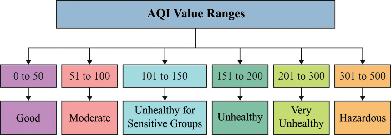
Figure 3: Ranges of AQI values

Tab. 1 and Figs. 4–6 shows the predictive results of the proposed OSSO-HDLAPM technique on test data. The results demonstrate that the proposed OSSO-HDLAPM technique accomplished proficient performance over other techniques. On the applied training dataset, CO was classified with an MAE of 0.108, MSE of 0.025, and an RMSE of 0.158.

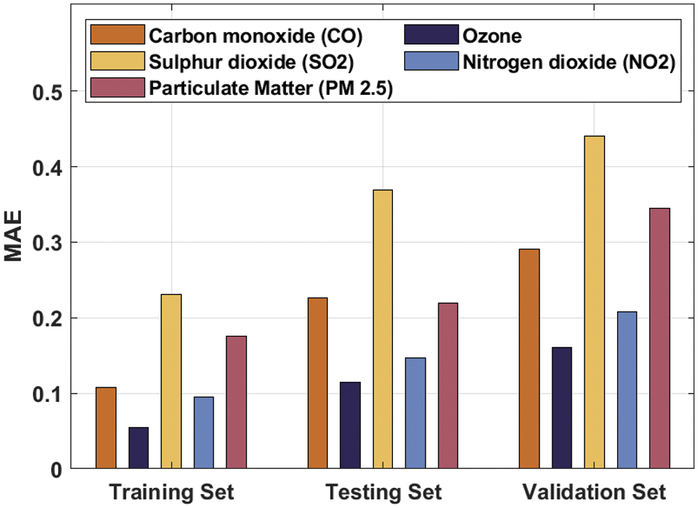
Figure 4: MAE analysis of OSSO-HDLAPM technique

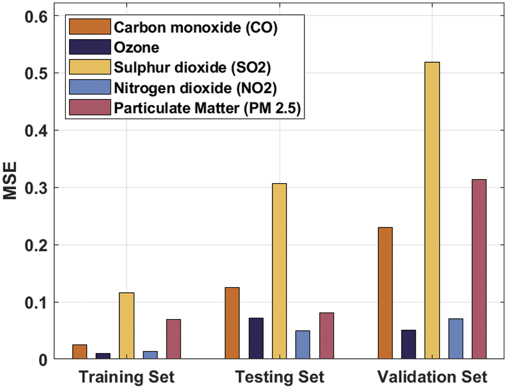
Figure 5: MSE analysis of OSSO-HDLAPM technique

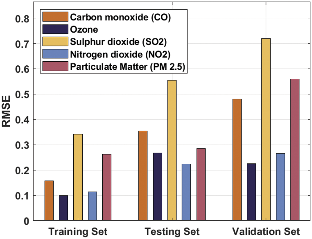
Figure 6: RMSE analysis of OSSO-HDLAPM technique

On the applied testing dataset, OSSO-HDLAPM technique attained an MAE of 0.226, MSE of 0.125, and an RMSE of 0.354. At the same time, on validation dataset, the proposed OSSO-HDLAPM technique gained an MAE of 0.291, MSE of 0.230, and an RMSE of 0.480. On the other hand, for training dataset, Ozone was classified with an MAE of 0.055, MSE of 0.010, and an RMSE of 0.100. Likewise, on the applied testing dataset, OSSO-HDLAPM technique attained an MAE of 0.115, MSE of 0.072, and an RMSE of 0.268. Similarly, on the validation dataset, the proposed OSSO-HDLAPM technique accomplished an MAE of 0.161, MSE of 0.051, and an RMSE of 0.226. Finally, on training dataset, PM 2.5 was classified with an MAE of 0.176, MSE of 0.069, and an RMSE of 0.263. Eventually, on the applied testing dataset, the proposed OSSO-HDLAPM technique gained an MAE of 0.219, MSE of 0.081, and an RMSE of 0.285. Meanwhile, for validation dataset, OSSO-HDLAPM technique resulted in an MAE of 0.345, MSE of 0.314, and an RMSE of 0.560.

Tab. 2 and Fig. 7 shows the results of analysis obtained by OSSO-HDLAPM technique under different training/testing datasets. The results show that the proposed OSSO-HDLAPM technique accomplished maximum predictive performance under distinct training/testing datasets. For instance, with training/testing dataset of 80:20 ratio, OSSO-HDLAPM technique obtained an increased precision of 98.56%, recall of 97.42%, accuracy of 97.80%, and an F-score of 97.99%. Moreover, with training/testing dataset of 80:20 ratio, the proposed OSSO-HDLAPM technique obtained an increased precision of 96.70%, recall of 94.37%, accuracy of 95.13%, and an F-score of 95.52%. Furthermore, in case of 80:20 training/testing dataset, OSSO-HDLAPM technique obtained an increased precision of 96.11%, recall of 92.98%, accuracy of 94.07%, and an F-score of 94.52%.

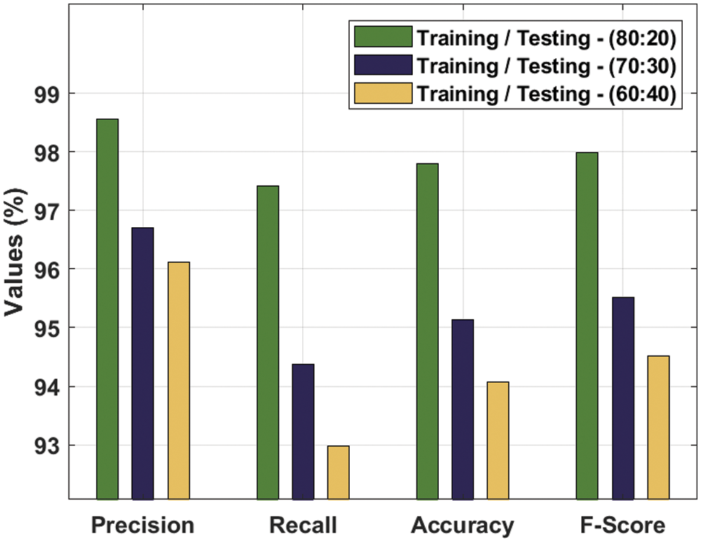
Figure 7: Predictive analysis results of OSSO-HDLAPM technique on varying training/testing sets

Finally, a comprehensive comparative analysis of OSSO-HDLAPM technique was conducted under different measures and the results are shown in Tab. 3. Fig. 8 shows the performance of the proposed OSSO-HDLAPM technique in terms of precision. The results demonstrate that PCA SVR (RBF Kernel) and SVR (RBF Kernel) techniques obtained the least precision values such as 61.50% and 62.30% respectively. Along with that, C4.5(DT) and ELM techniques produced moderate precision values namely, 93.20% and 94.60% respectively. In line with these, MLP model gained a competitive precision of 94.60%. However, the presented OSSO-HDLAPM technique resulted in a maximum precision of 98.56%.

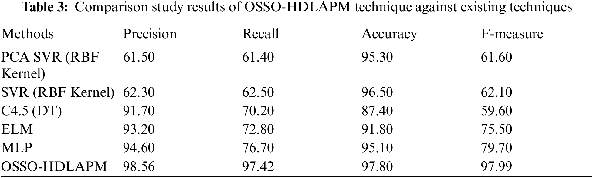
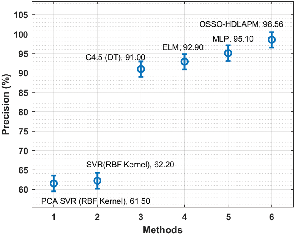
Figure 8: Precision analysis of OSSO-HDLAPM technique

Fig. 9 shows the outcomes of the proposed OSSO-HDLAPM technique in terms of recall. The obtained values highlight that PCA SVR (RBF Kernel) and SVR (RBF Kernel) techniques attained low recall values such as 61.50% and 62.30% respectively. Then, C4.5(DT) and ELM techniques accomplished reasonable recall values such as 93.20% and 94.60% respectively. Next, MLP model accomplished a near optimum recall of 94.60%. But the presented OSSO-HDLAPM technique outperformed earlier models with a supreme recall of 98.56%.

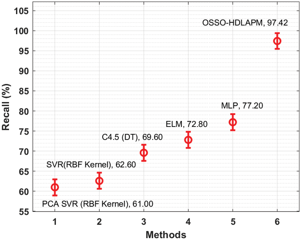
Figure 9: Recall analysis of OSSO-HDLAPM technique

Fig. 10 shows the results offered by OSSO-HDLAPM technique in terms of accuracy. The figure showcase that both PCA SVR (RBF Kernel) and SVR (RBF Kernel) techniques gained the least accuracy values such as 61.50% and 62.30% respectively. Moreover, C4.5(DT) and ELM techniques produced manageable accuracy values being 93.20% and 94.60% respectively. Furthermore, MLP model depicted a competitive accuracy of 94.60%. However, the presented OSSO-HDLAPM technique surpassed existing techniques and achieved a high accuracy of 98.56%.

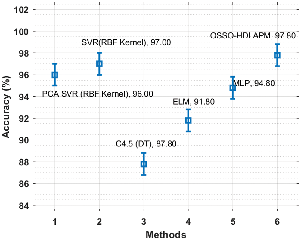
Figure 10: Accuracy analysis of OSSO-HDLAPM technique

Finally, the outcomes of the comparative study conducted between the proposed OSSO-HDLAPM technique and other techniques in terms of F-measure report that PCA SVR (RBF Kernel) and SVR (RBF Kernel) techniques portrayed poor results with F-measure values such as 61.50% and 62.30% respectively. Concurrently, C4.5(DT) and ELM techniques too resulted in moderate F-measure values alike 93.20% and 94.60% respectively. Simultaneously, MLP model gained a competitive F-measure of 94.60%. However, the presented OSSO-HDLAPM technique produced a maximum F-measure of 98.56%. From the discussion made above for the analysis and results, it is clear that the proposed OSSO-HDLAPM technique can be used as an effective tool to monitor air pollution in ITS environment.

5  Conclusion

In this study, a new OSSO-HDLAPM technique is designed to monitor the air pollution in ITS environment. To boost the convergence rate of SSO algorithm, OBL concept is employed which enhances the quality of initial population solution. The proposed OSSO-HDLAPM technique deploys an array of sensors in the vehicles to measure the level of pollutants. This information is then transmitted to cloud environment for further processing. Moreover, HCNN-LSTM based prediction and OSSO-based hyperparameter optimization processes also are executed. Finally, in order to validate the efficacy of the proposed OSSO-HDLAPM technique, a sequence of experimentations was accomplished and the results were examined under dissimilar aspects. The resultant experimental outcomes highlight the better performance of OSSO-HDLAPM technique over recent state-of-the-art approaches. In future, the predictive outcome can be enhanced by the incorporation of feature selection approaches.

Funding Statement: The authors received no specific funding for this study.

Conflicts of Interest: The authors declare that they have no conflicts of interest to report regarding the present study.

References

 1.  A. Haydari and Y. Yilmaz, “Deep reinforcement learning for intelligent transportation systems: A survey,” IEEE Transactions on Intelligent Transportation Systems, vol. 23, no. 1, pp. 1–22, 2020. [Google Scholar]

 2.  F. Arena, G. Pau and A. Severino, “A review on IEEE 802.11 p for intelligent transportation systems,” Journal of Sensor and Actuator Networks, vol. 9, no. 2, pp. 22, 2020. [Google Scholar]

 3.  S. Wan, X. Xu, T. Wang and Z. Gu, “An intelligent video analysis method for abnormal event detection in intelligent transportation systems,” IEEE Transactions on Intelligent Transportation Systems, vol. 22, no. 7, pp. 4487–4495, 2021. [Google Scholar]

 4.  M. Abbasi, M. Rafiee, M. R. Khosravi, A. Jolfaei, V. G. Menon et al., “An efficient parallel genetic algorithm solution for vehicle routing problem in cloud implementation of the intelligent transportation systems,” Journal of Cloud Computing, vol. 9, no. 1, pp. 6, 2020. [Google Scholar]

 5.  I. V. Pustokhina, D. A. Pustokhin, J. J. Rodrigues, D. Gupta, A. Khanna et al., “Automatic vehicle license plate recognition using optimal k-means with convolutional neural network for intelligent transportation systems,” IEEE Access, vol. 8, pp. 92907–92917, 2020. [Google Scholar]

 6.  M. Zichichi, S. Ferretti and G. D'angelo, “A framework based on distributed ledger technologies for data management and services in intelligent transportation systems,” IEEE Access, vol. 8, pp. 100384–100402, 2020. [Google Scholar]

 7.  A. K. Haghighat, V. R. Mouli, P. Chakraborty, Y. Esfandiari, S. Arabi et al., “Applications of deep learning in intelligent transportation systems,” Journal of Big Data Analytics in Transportation, vol. 2, no. 2, pp. 115–145, 2020. [Google Scholar]

 8.  A. A. Dweik, R. Muresan, M. Mayhew and M. Lieberman, “IoT-based multifunctional scalable real-time enhanced road side unit for intelligent transportation systems,” in 2017 IEEE 30th Canadian Conf. on Electrical and Computer Engineering (CCECE), Windsor, ON, Canada, pp. 1–6, 2017. [Google Scholar]

 9.  S. Kaivonen and E. C. -H. Ngai, “Real-time air pollution monitoring with sensors on city bus,” Digital Communications and Networks, vol. 6, no. 1, pp. 23–30, 2020. [Google Scholar]

10. S. O. Ogundoyin, “An anonymous and privacy-preserving scheme for efficient traffic movement analysis in intelligent transportation system,” Security and Privacy, vol. 1, no. 6, pp. e50, 2018. [Google Scholar]

11. T. Shen, K. Hua and J. Liu, “Optimized public parking location modelling for green intelligent transportation system using genetic algorithms,” IEEE Access, vol. 7, pp. 176870–176883, 2019. [Google Scholar]

12. M. A. Mondal and Z. Rehena, “Intelligent traffic congestion classification system using artificial neural network,” in Companion Proc. of The 2019 World Wide Web Conf., San Francisco, USA, pp. 110–116, 2019. [Google Scholar]

13. B. Vamshi and R. V. Prasad, “Dynamic route planning framework for minimal air pollution exposure in urban road transportation systems,” in 2018 IEEE 4th World Forum on Internet of Things (WF-IoT), Singapore, pp. 540–545, 2018. [Google Scholar]

14. J. Xie and Y. K. Choi, “Hybrid traffic prediction scheme for intelligent transportation systems based on historical and real-time data,” International Journal of Distributed Sensor Networks, vol. 13, no. 11, pp. 155014771774500, 2017. [Google Scholar]

15. C. Shetty, B. J. Sowmya, S. Seema and K. G. Srinivasa, “Air pollution control model using machine learning and IoT techniques,” In Advances in Computers, vol. 117, no. 1, pp. 187–218, 2020. [Google Scholar]

16. W. He, J. Li, Z. Tang, B. Wu, H. Luan et al., “A novel hybrid cnn-lstm scheme for nitrogen oxide emission prediction in fcc unit,” Mathematical Problems in Engineering, vol. 2020, pp. 1–12, 2020. [Google Scholar]

17. A. Krizhevsky, I. Sutskever and G. E. Hinton, “ImageNet classification with deep convolutional neural networks,” Communications of the ACM, vol. 60, no. 6, pp. 84–90, 2017. [Google Scholar]

18. L. Wang, X. Wang, Z. Sheng and S. Lu, “Multi-objective shark smell optimization algorithm using incorporated composite angle cosine for automatic train operation,” Energies, vol. 13, no. 3, pp. 714, 2020. [Google Scholar]

19. M. Ahmadigorji and N. Amjady, “A multiyear DG-incorporated framework for expansion planning of distribution networks using binary chaotic shark smell optimization algorithm,” Energy, vol. 102, pp. 199–215, 2016. [Google Scholar]

20. P. Anitha and B. Kaarthick, “Oppositional based Laplacian grey wolf optimization algorithm with SVM for data mining in intrusion detection system,” Journal of Ambient Intelligence and Humanized Computing, vol. 12, no. 3, pp. 3589–3600, 2021. [Google Scholar]

This work is licensed under a Creative Commons Attribution 4.0 International License, which permits unrestricted use, distribution, and reproduction in any medium, provided the original work is properly cited.