DOI:10.32604/cmc.2022.024356
| Computers, Materials & Continua DOI:10.32604/cmc.2022.024356 | |
| Article |
Efficiency Effect of Obstacle Margin on Line-of-Sight in Wireless Networks
1Department of Electrical Engineering–Communication Engineering, Sana'a University, 61101, Yemen
2Department of Information Systems-Girls Section, King Khalid University, Mahayil, 62529, Saudi Arabia
3Department of Computer Science, King Khalid University, Muhayel Aseer, 62529, Saudi Arabia
4Faculty of Computer and IT, Sana'a University, Sana'a, 61101, Yemen
5Department of Information Systems, King Khalid University, Muhayel Aseer, 62529, Saudi Arabia
6Department of Computer and Self Development, Preparatory Year Deanship, Prince Sattam bin Abdulaziz University, AlKharj, 16278, Saudi Arabia
*Corresponding Author: Manar Ahmed Hamza. Email: ma.hamza@psau.edu.sa
Received: 14 October 2021; Accepted: 03 December 2021
Abstract: Line-of-sight clarity and assurance are essential because they are considered the golden rule in wireless network planning, allowing the direct propagation path to connect the transmitter and receiver and retain the strength of the signal to be received. Despite the increasing literature on the line of sight with different scenarios, no comprehensive study focuses on the multiplicity of parameters and basic concepts that must be taken into account when studying such a topic as it affects the results and their accuracy. Therefore, this research aims to find limited values that ensure that the signal reaches the future efficiently and enhances the accuracy of these values’ results. We have designed MATLAB simulation and programming programs by Visual Basic .NET for a semi-realistic communication system. It includes all the basic parameters of this system, taking into account the environment's diversity and the characteristics of the obstacle between the transmitting station and the receiving station. Then we verified the correctness of the system's work. Moreover, we begin by analyzing and studying multiple and branching cases to achieve the goal. We get several values from the results, which are finite values, which are a useful reference for engineers and designers of wireless networks.
Keywords: Line of sight; obstacle margin; wireless networks; communication link; radio wave propagation
The process of having an unobstructed line of sight (LOS) between the transmitter antenna and the receiving antenna between them is a fundamental basis for designing the RF link. The direct path of the electromagnetic waves between the transmitter and receiver is called the LOS propagation path. This explicit path is the communication link of radio frequency (RF), and at the same time, it contains the bulk of the received signal in the receiving antenna [1–3]. It must meet the condition that there are no obstacles or blocking the direct propagation path so that the signal level is not affected. Therefore, it is typical for the propagation path to encounter physical elements (mountains, buildings, metal structures, and other obstacles). Involves the signal level or signal interruption. Even water bodies and the overlapping terrain surface influence the propagation path [4]. The phenomenon of the sum of the phase angle and the amplitude of the electric fields, and if the sum of the wave waves reaches zero, the signal is not received [5–8].
When designing the RF links and several analyzes and procedures implemented, one of the necessary analyzes and calculations (free space loss, link budget, rain attenuation, multi-path fade, fade margin, and Fresnel zones) is performed before fixation of the microwave link [9–13].
In recent years, there has been a fair amount of line-of-sight literature, for example, a propagation prediction technique for predicting propagation mechanisms for fixed line-of-sight radio links, remarkably proposed for rural environments. They report a short-term prevalence measurement campaign that has been carried out in the Ankara region, Turkey. Field measurements were performed at a frequency of 2.536 GHz for three months in summer 2015. It notes that the difference between the measurement data and the expected average received power is less than the standard deviation value provided in Recommendation ITU-R P. 1546. And [14], it has been observed that the state of LOS influences the atmospheric factor, causing a critical signal loss. The different propagation loss mechanisms are also briefly described on the Link Balancing Tool (LBT). It can determine the effect of signal loss and expected performance according to the distances between link propagation conditions based on many system parameters.
From the above, it is clear that the signal strength and attenuation are greatly influenced by the nominal range or the distance between the transmitters. From this standpoint, the research aims to analyze and study the most critical factors that affect the line of sight. It is the effect of the obstacle margin and its impact, finding solutions, and knowing the characteristics of the signal when it is present in several forms, considering the parameters and communication link through the design and simulation [15–20]. All these parameters (more than nineteen transactions and obtain ten results) design, develop, manipulate, or predict the signal's behavior in multiple frameworks for environmental conditions to achieve accurate results that enhance the importance of this research.
The remainder of the article is structured. In Section 2, we explain the proposed system model. Implementation and simulation are provided in Section 3. Results analysis and discussion are provided in Section 4, and finally, we conclude the article in Section 5.
Suppose a system model has four core parts are analyses of the relationship between occlusion and antenna heights, analysis of the relationship between the length of the antennas, analysis of the effect of building loss on margin, and a multi-track margin and fades analysis.
The first part is focusing on analyses the relationships between occlusion height and antenna heights for the diagnosis of three cases; the obstacle height is smaller than the antennas, the obstacle height is equal to that of each antenna, and the obstacle height is equal to the length of one of the antennas and the other antenna is smaller or the obstacle is greater than the two of them.
The second part provides an analysis of the relationship between the length of the first antenna and the second antenna with the value of the margin. The third part introduces the effect of building loss on margin for diagnosing two situations; the length of the obstacle is changed and building loss 20 and 10 dB. The fourth part provides a multi-track margin and fades analysis of third cases; Free-Space-Path loss, values calculated for the three links (900 MHz, 2.4, and 5.8 GHz), the minimum signal-to-noise ratio required to satisfy data rates of Binary Phase-shift keying (BPSK), Quadrature Phase Shift Keying (QPSK), and Quadrature Amplitude Modulation (QAM) (BPSK 1/2, BPSK 3/4, QPSK 1/2, QPSK 3/4, QPSK 3/4, 16-QAM 1/2, 16-QAM 3/4, 64-QAM 2/3, 64-QAM 3/4), and the data rates vs. estimated maximum distance.
The communication system model has been designed, implemented, and simulated using a self-developed program and simulation software. They consist of the main parameters for developing a communication system, consisting of two main parts (values and variables for receivers, transmitters, deals, and variables related to the surrounding environment, etc.), to achieve accurate results that enhance the importance of this research. Fig. 1 illustrates the general structure of the system model.
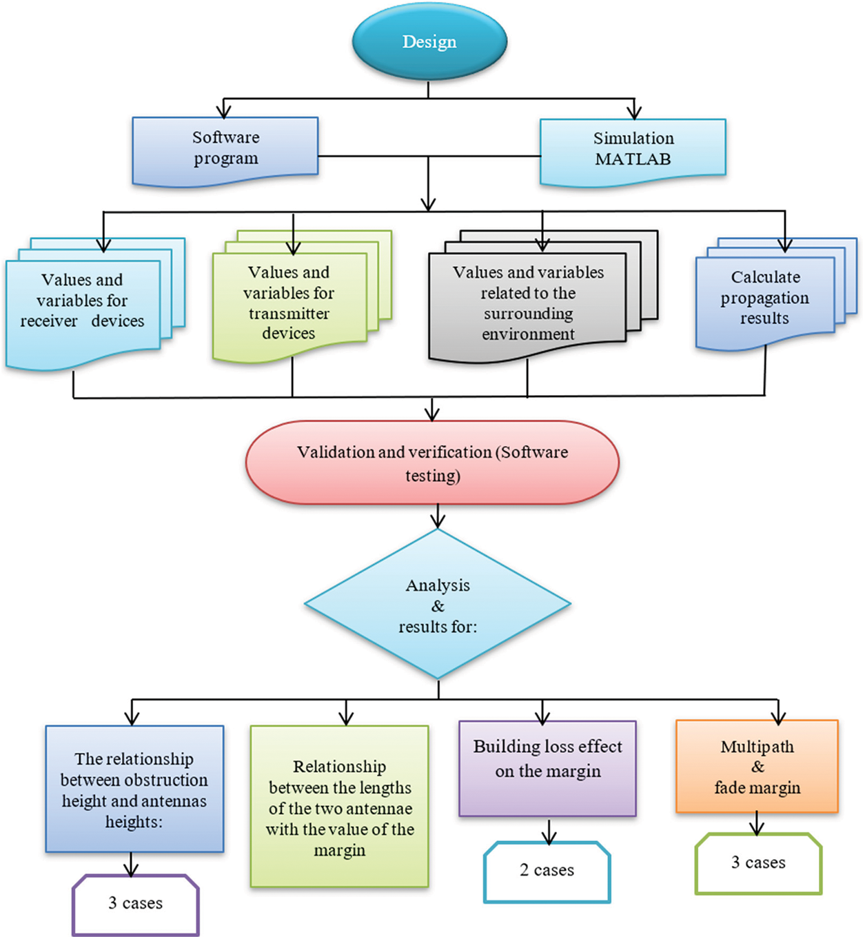
Figure 1: The main components of the proposed system model
3 Implementation and Simulation
To calculate the radio wave propagation and evaluate the effect of obstacle margin on line-of-sight and its effect on the efficiency of wireless communication, the self-developed software has been developed using Visual Basic.net programming language. The simulated software has been developed using MATLAB environment. This section explains in detail the developed and simulation software. Fig. 2 shows the core parameters of the developed software of the proposed system model.
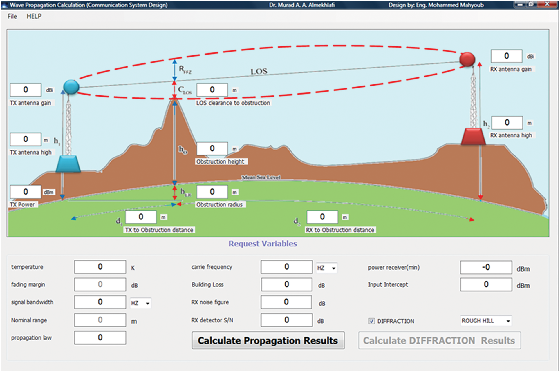
Figure 2: The core parameters of the developed software of the proposed system model
The developed software contains a control panel to set up the initial parameters that control the spread of waves. It can be modified to reach the desired result to ensure the quality of the transmission and reception of the communication system. The components of the proposed model of the communication system can be categorized into three main parts as follow:
- Parameters of the receiver and transmitter devices.
- Parameters related to the surrounding environment.
- Parameters for calculation of the propagation results.
The following subsections explain in detail all these parts.
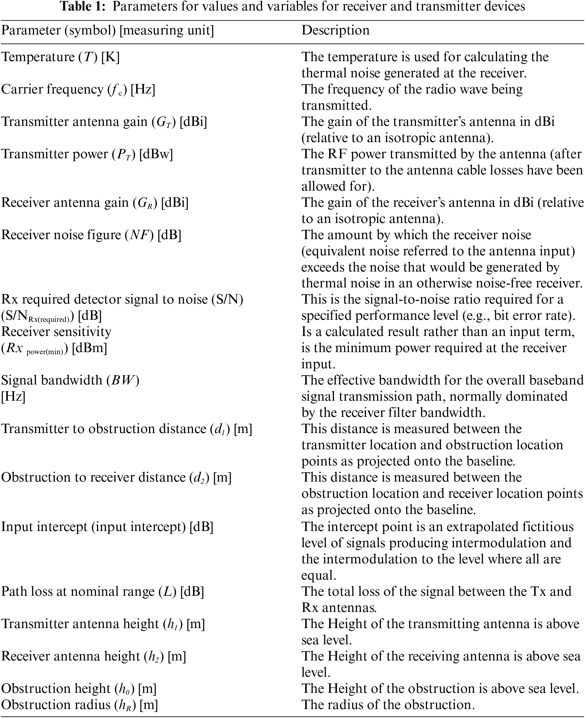
3.1 Parameters of the Receiver and Transmitter Devices
This subsection explains the parameters for values and variables of receiver and transmitter devices as shown in Tab. 1.
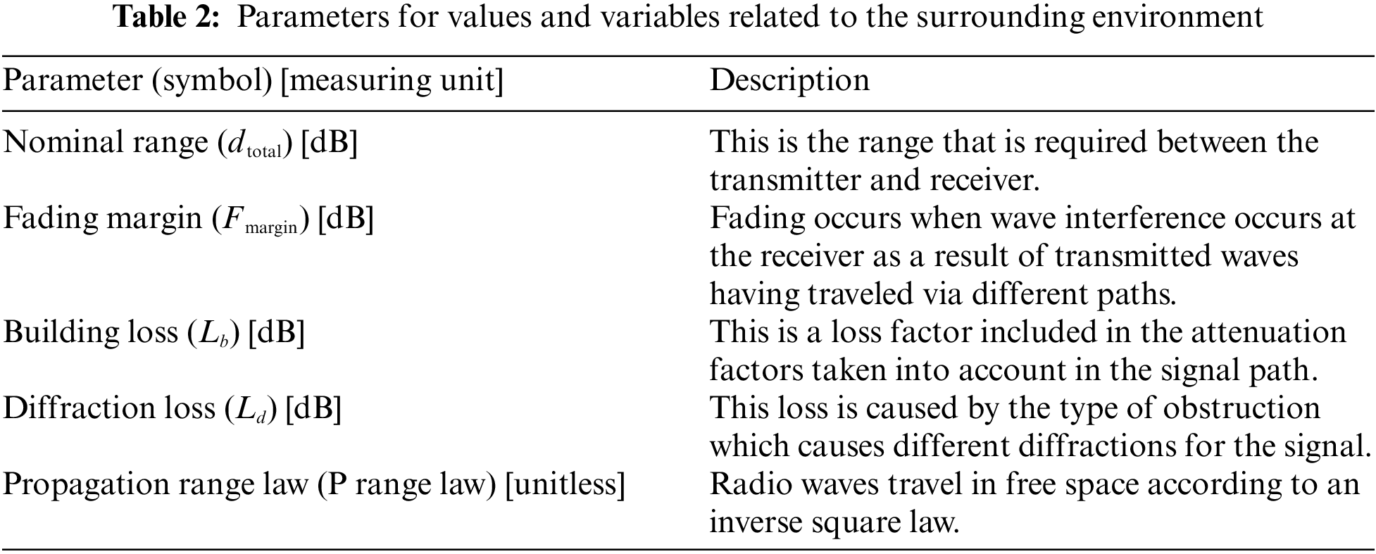
3.2 Parameters Related to the Surrounding Environment
This subsection explains the parameters for values and variables related to the surrounding environment are shown in Tab. 2.
3.3 Parameters for the Calculation the Propagation Results
This subsection presents the parameters required as inputs for calculation of the propagation results of the proposed telecommunications system as shown in Tab. 3.
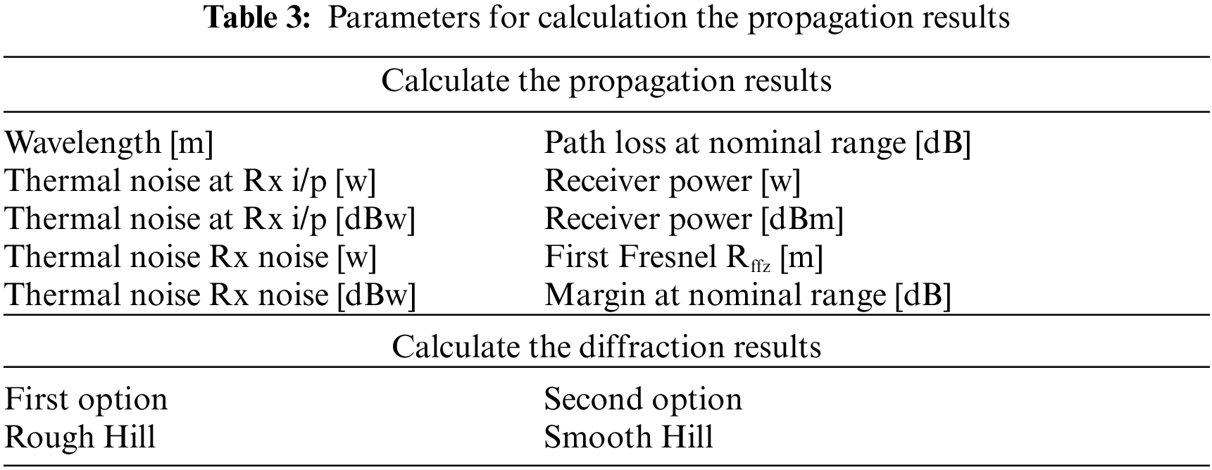
Fig. 3 illustrates the core parameters for the calculation of the propagation results of the proposed telecommunications system.
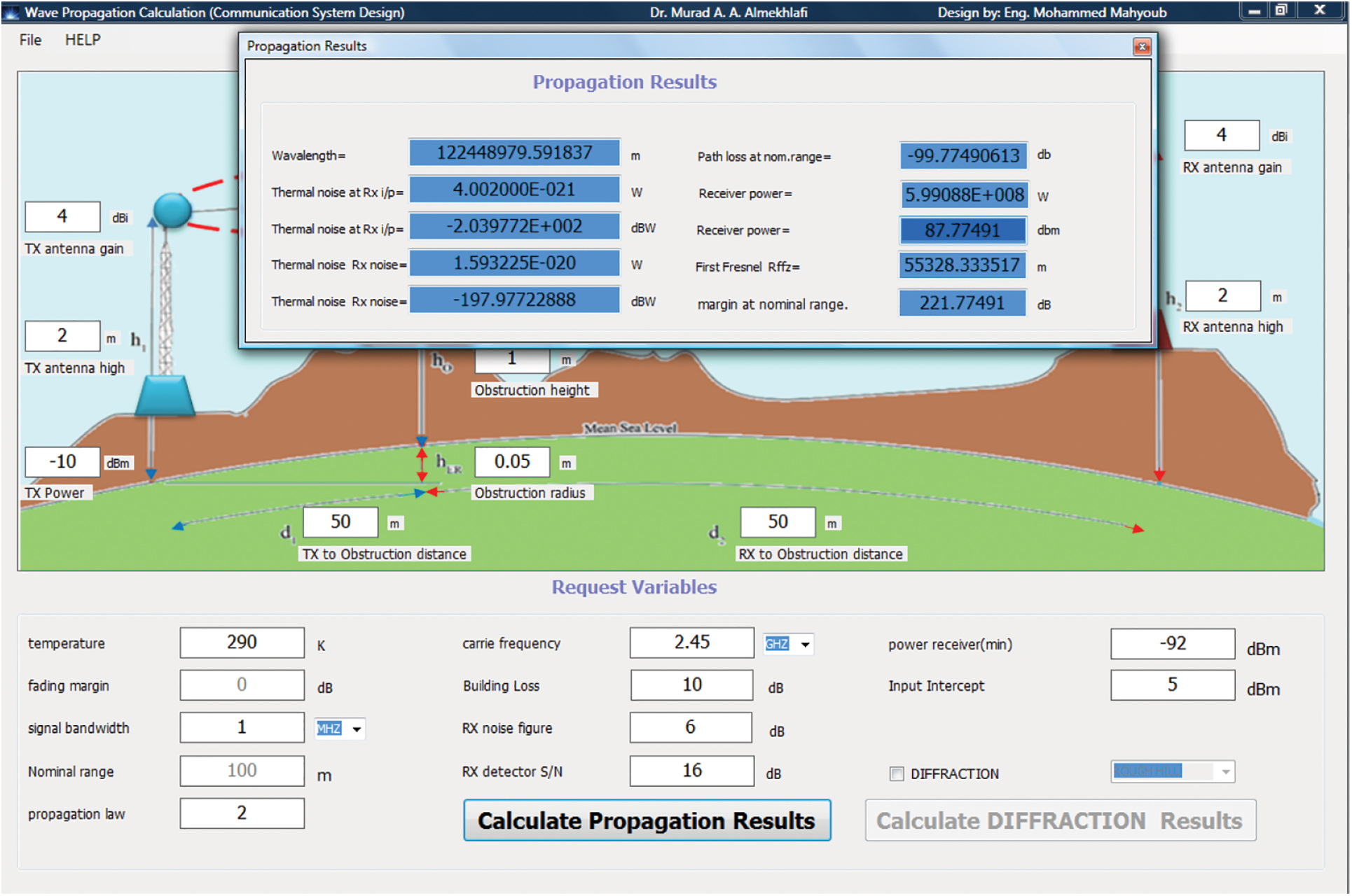
Figure 3: The core parameters for calculation of the propagation results of the proposed system
The multiplication of results values in the program proves the accuracy of the results and the size of the program. Also, the values of the program inputs to design a communication link enhance the size and quality of the wireless communication link to be designed [21–23].
Here we can say the main rule when determining that the communication link is sufficient to transmit data under perfect conditions if the resigned power is enormous about the receiver sensitivity.
The obstacle of the proposed system and the simulation software represents a mountain, a building, or a house, etc. Assuming an isotropic antenna (the gain is zero) and the rest of the parameters and their related values are built into the developed software of the proposed communication system are shown in Tab. 4.
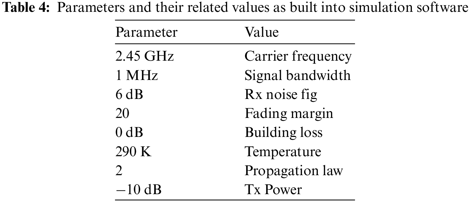
The parameters values shown in Tab. 4 above are assumed in the following three cases:
- In the first case, we think that the height of the obstacle is smaller than the two antennas.
- In the second case, we assume that the height of the barrier is equal to the lengths of the two antennas.
- In the third case, we believe that the obstacle height is similar to the length of one of the antennas, and the other antenna is smaller, or the obstacle is more significant than the two of them.
4.1 Case 1: The Obstacle Height is Smaller than the Antennas
Assuming that the nominal range is 100 m, the noise figure of the receiver equals 6 dB and the length of both antennas is the same and longer than the length of the obstacle as follows:
- Nominal range: dtotal = 100 m.
- Noise figure: NF = 6 dB.
- Transmitting antenna height: h1 = 2 m.
- Receiving antenna height: h2 = 2 m.
- Obstacle height: ho = 1 m.
The location of the obstacle has been changed and the provided results are shown in Tab. 5.
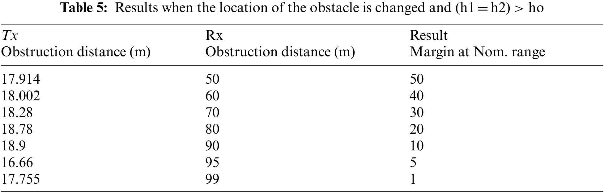
At the nominal range, the value of the margin changes by the location of the obstacle (only if it is length is smaller than the length of the antenna), and it is independent of the smoothness of the obstacle (soft or rough), so it gives the same results for the soft or rough obstacle. The highest value for the margin is obtained at (Tx, Rx) = (20, 80) or (80, 20). As we see, there is no difference whether the distance 20 m is between the obstacle and the transmitter or between the obstacle and the receiver. Both give the same results for the margin. Also, we note that when the obstacle approaches the sending or receiving antennas, the values of the margin swing up and fall back at (Tx, Rx) = (1, 99). Still, practically this is unviable because no obstacle can be placed in this arrangement.
4.2 Case 2: The Obstacle Height is Equal to that of Each Antenna
Assuming the previous initial conditions for case1 but this time the height of the obstacle is the same as the antennas as follows:
- Nominal range: dtotal = 100 m.
- Noise figure: NF = 6 dB.
- Transmitting antenna height: h1 = 2 m.
- Receiving antenna height: h2 = 2 m.
- Obstacle height: ho = 2 m.
The location of the obstacle has been changed and the provided results are shown in Tab. 6.
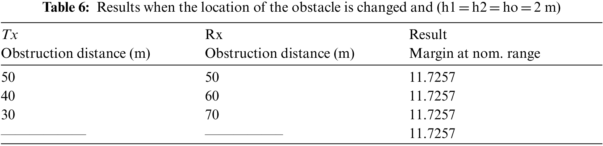
From the results shown in Tab. 6 above, we conclude that the value of the margin did not change with the obstacle's location. It remained constant because the height of both the antennae and the barrier is equal. The obstacle width does not affect the margin because the obstacle height is similar or smaller than the antenna. Again, in this case, the margin value is independent of the obstacle's smoothness, soft or rough, so it gives the same results for a smooth or rough barrier.
4.3 Case 3: The Obstacle Height is Equal to the Length of One of the Antennas and the Other Antenna is Smaller or the Obstacle is Greater Than the Two of Them
Assuming the initial conditions for case1 but this time the obstacle height is equal to the length of one of the antennas and the other antenna is smaller, or the obstacle is greater than the two of them as follows:
- Nominal range: dtotal = 100 m.
- Noise figure: NF = 6 dB.
- Transmitting antenna height: h1 = 2 m.
- Receiving antenna height: h2 = 1 m or h2 = 2 m.
- Obstacle height: ho = 2 m or ho = 4 m.
The results of this case can be summarized as follows:
- A change in the location of the obstacle between the transmitter and receiver changes the value of the margin.
- The margin value is dependent on the smoothness of the impediment to the soft or coarse surface.
- The rough surface gives a more considerable margin than the smooth surface because the rough surface can make several refractories and reflections.
- The margin is different from the width of the barrier (Radius), which is inversely proportional to the width of the barrier.
4.4 The Relationship Between the Length of the First Antenna and the Second Antenna with the Value of the Margin
Assuming that, the length of the transmitting antenna equals 2 meters, which is proven on the whole experiment to study the length ratio of the receiving antenna, which will give the largest value of the margin as shown in Tab. 7.
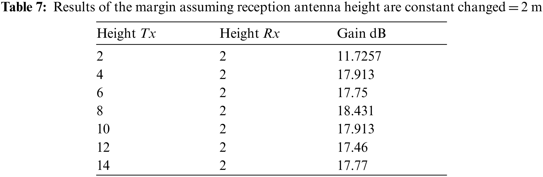
Note that the most massive value of the margin is obtained when the ratio of the length of the first antenna to the second antenna is equal to 8/2, and this means that the wavelength equals four.
4.5 Building Loss Effect on the Margin
The loss factor here includes attenuation coefficients taking into account the path of the signal. For an unobstructed direct line of sight, the building loss factor can be set to zero. The loss of penetration from inside to outside the wall is measured. Reference [24] provides detailed maps of substantial multi-story buildings, low-rise concrete construction, and building structures. Tab. 8 summarizes these results.

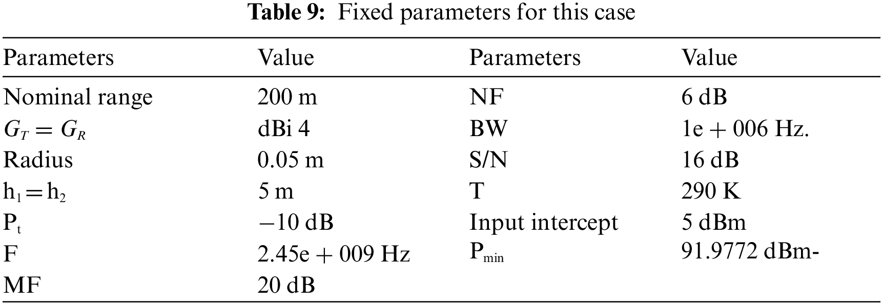
The sample of standard deviations varies in these surveys but is generally less than or equal to 10.3 dB as shown in Tab. 9.
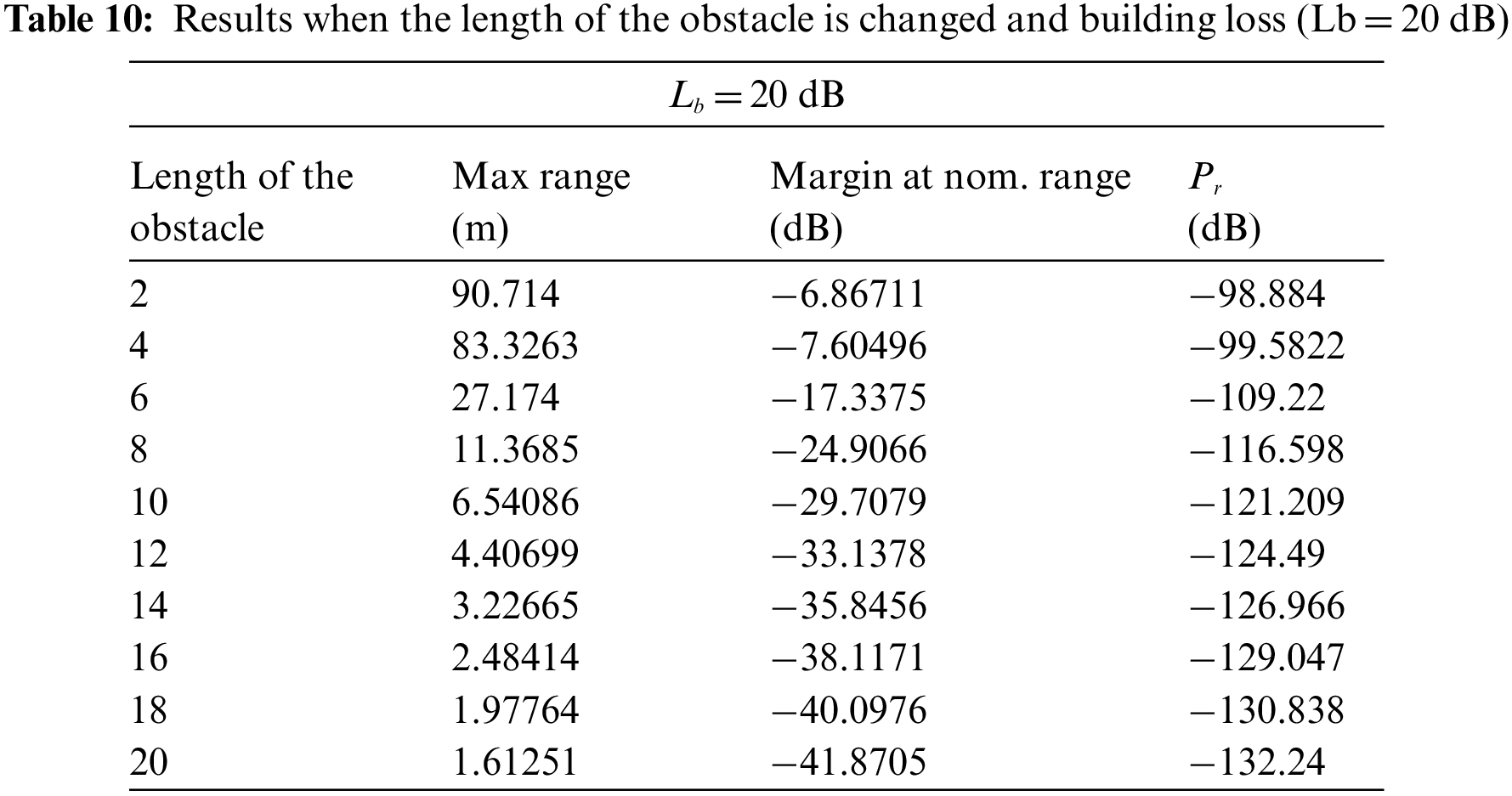
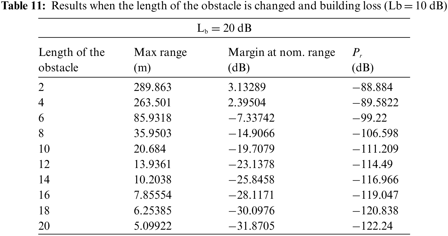
As the obtained results are shown in Tabs. 10 and 11 above, the results can be summarized as follows:
- The more significant the building loss (Lb), the higher loss the signal will encounter.
- The more significant the Lb, the less energy received.
- The more significant the length of the obstacle, the less energy received.
- When Lb was more massive, although the height of the barrier was less than the length of the antenna, there was no reception of the transmitted energy.
- When Lb decreases to 10 dB, there is a decrease in the margin at nom. range by the same amount.
- If the length of an antenna varies, we notice a slight decrease in the transmitted power.
It is also known that when the waves travel in different paths than the direct line-of-sight path, which often causes the waves’ interference or causes the problem of vanishing when the different paths of the waves end with the exit of the phase angle and cancel each other. There are several solutions to this problem; the most important of them (changing the antenna location or increasing the power capacity), these and other solutions reduce multipath. The addition of the amount of wireless energy that is radiated by the transmitter to overcome the fading margin phenomenon must be accurate.
To obtain the exact amount of fade margin for the wireless link, we will analyze several things, which can be summarized in five arithmetic stages (Free-Space-Path loss (PLFSPL), Received Power, Signal-to-Noise Ratio (SNR), Maximum Channel Noise, and Check Link Margin by Rayleigh's Fading Model). All of these stages (calculations) to find the required reliability of the link is to maintain (20 dB) to (30 dB) from the fade margin at all times. Fig. 4 shows the Free-Space-Path loss (PLFSPL), values calculated for the three links (900 MHz, 2.4, and 5.8 GHz).
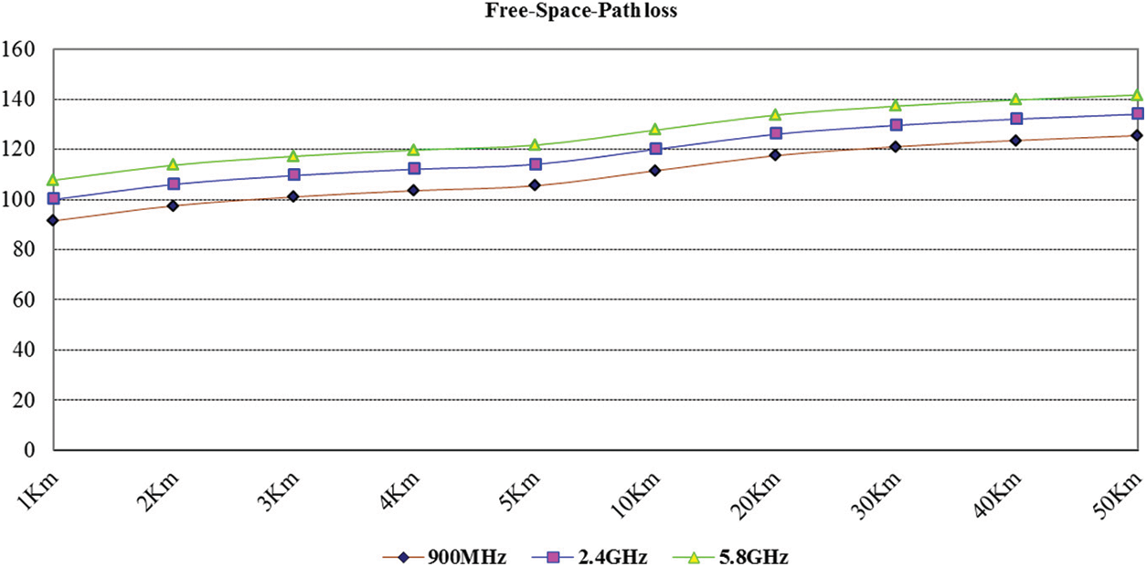
Figure 4: The values of free-space-path loss
The other losses in the radio system must be taken into account when designing the network and calculating its budget. These losses are in the antenna cables and connectors, which were calculated with units Transco's integrated to use integrated antennas. It was a loss (0.25 dB) for each conductor and a loss (0.25 dB) for every three meters of the station antenna type (LMR 400), which should be a loss (0.75 dB) included for every three meters according to the manual and specifications for the cable type and system design.
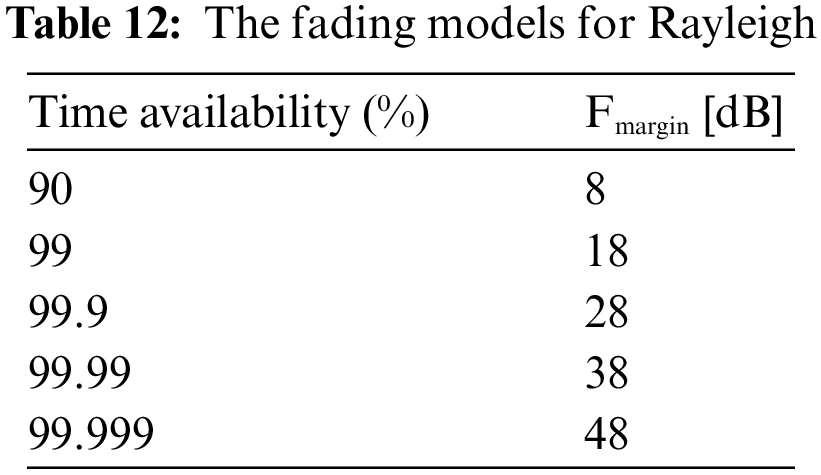
Tab. 12 shows the Rayleigh Fading model, which shows the relationship between the available margin of correlation and the correlation of availability.
An essential aspect of determining system reliability is the signal-to-noise ratio (SNR) of the given modulation technique. It achieves a certain level of reliability in the receiving station error rate (BER) conditions. We find that there is always a comparison between data rates and distance. When comparing, for example, between (64-QAM) and (BPSK), we find that (64-QAM) requires a more excellent (SNR) ratio and it is, of course, considered more efficient compared to (BPSK) which requires a ratio ( SNR) is lower, as it is more resistant to channel noise.
Therefore, calculations were made to know the minimum signal-to-noise ratio required to satisfy data rates, as shown in Tab. 13.

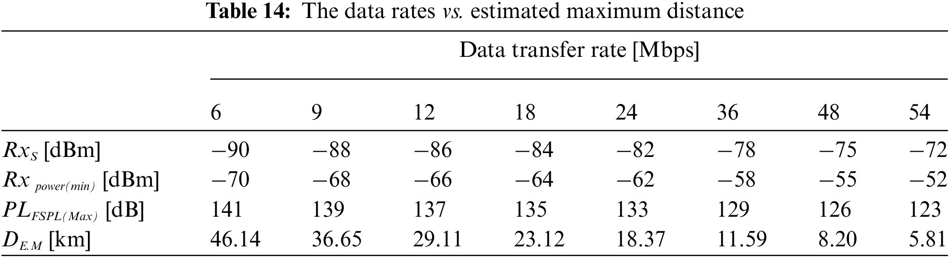
Since the radio received sensitivity varies according to the different modulation and data transfer rates. Therefore, it is calculated with the determination of the estimated maximum distance (DE.M), Receiver Sensitivity (RxS), minimum received power (Rxpower(min)), and maximum free-space path loss (PLFSPL(Max)), as shown in Tab. 14.
This work aims to analyze and study the effect of the obstacle on a line of sight. As indicated by the results, the nominal range hurts the reception. With the large frequencies, the higher the barrier is the lower the communication efficiency, and the lower the communication efficiency. In the middle is the Link. This medium contains several factors such as rain, dust, and fog, forcing us to increase the dwindling margin, i.e., increases the difference between the transmitted power and the minimum power required to be sent. When the building loss decreases to 10 dB, there is a decrease in the margin at nom. range by the same amount. If the length of an antenna varies, we notice a slight reduction in the transmitted power. Also, the signal-to-noise ratio has been determined for each of the different data rates, and the maximum distance has been selected for the lowest receiving reception capacity. The other results constitute a guide for designers of the wireless communication system concerning point-to-point Link. The software program design is not the main subject of this research, as indicated by this research title. Still, it is considered an auxiliary part, and we will develop the program in several aspects, and it will be published as independent research.
Funding Statement: The authors extend their appreciation to the Deanship of Scientific Research at King Khalid University for funding this work under Grant Number (RGP 1/282/42), https://www.kku.edu.sa.
Conflicts of Interest: The authors declare that they have no conflicts of interest to report regarding the present study.
1. H. Arafat and M. Sangman, “Wireless channel models for over-the-sea communication: A comparative study,” MDPI Applied Sciences, vol. 9, pp. 1–32, 2019. [Google Scholar]
2. A. Habib and S. Moh, “A survey on channel models for radio propagation over the sea surface,” in Proc. of the 10th Int. Conf. on Internet (ICONI 2018), Phnom Penh, Cambodia, 2018. [Google Scholar]
3. Y. Lee, F. Dong and Y. Meng, “Stand-off distances for non-line-of-sight maritime mobile applications in 5 GHZ band,” Progress in Electromagnetics Research B, vol. 54, pp. 321–336, 2013. [Google Scholar]
4. G. Polat, T. Satilmis, K. Ezhan and A. Ayhan, “The effect of multipath fading on terrestrial microwave line-of-sight (LOS) radio links,” in IEEE Int. Symp. on Antennas and Propagation & USNC/URSI National Radio Science Meeting, Vancouver, BC, Canada, 2015. [Google Scholar]
5. Z. Nadir, M. Suwailam and M. Idrees, “Pathloss measurements and prediction using statistical models,” in 7th Int. Conf. on Mechanical, Industrial, and Manufacturing Technologies (MIMT 2016MATEC Web of Conferences, vol. 54, South Africa, pp. 1–4, 2016. [Google Scholar]
6. S. Peter, “Antennas and electromagnetic wave propagation: Radar, seekers and sensors, tracking, and target recognition,” Encyclopedia of Aerospace Engineering, vol. 15, 2010. [Google Scholar]
7. J. Wenyi, K. Guan, Z. Zhangdui, A. Bo, H. Ruisi et al., “Propagation and wireless channel modeling development on wide-sense vehicle-to-x communications,” International Journal of Antennas and Propagation, vol. 2013, pp. 1–11, 2013. [Google Scholar]
8. Y. Guo, J. Zhang, C. Tao, U. Liu and L. Tian, “Propagation characteristics of wideband high-speed railway channel in viaduct scenario at 2. 35 GHz,” Journal of Modern Transportation, vol. 20, pp. 206–212, 2012. [Google Scholar]
9. H. Lehpamer, Microwave Transmission Network. Second edition, ISBN: 0071701222, McGraw-Hill Professional, US, 2012. [Google Scholar]
10. B. Ai, R. He and Z. Zhong, “Radio wave propagation scene partitioning for high-speed rails,” International Journal on Antennas and Propagation, vol. 2012, pp. 1–7, 2012. [Google Scholar]
11. K. Guan, Z. Zhong, B. Ai and T. Kuerner, “Semi-deterministic propagation modeling for high-speed railway,” IEEE Antennas and Wireless Propagation Letters, vol. 12, pp. 789–792, 2013. [Google Scholar]
12. K. Guan, Z. Zhong, B. Ai and C. Rodríguez, “Modeling of the division point of different propagation mechanisms in the near-region within arched tunnels,” Wireless Personal Communications, vol. 68, pp. 489–505, 2013. [Google Scholar]
13. K. Guan, Z. Zhong and B. Ai, “Complete propagation model structure inside tunnels,” Progress in Electromagnetics Research, vol. 141, pp. 711–726, 2013. [Google Scholar]
14. H. Anwar, F. Mohammed, S. Mohammed, S. Abdulrahman and I. Muhammed, “Link budget design for RF line-of-sight via theoretical propagation prediction,” International Journal of Communications, Network and System Sciences, vol. 12, pp. 11–17, 2019. [Google Scholar]
15. K. Guan, Z. Zhong, B. Ai, R. He and C. Rodriguez, “Five-zone propagation model for large-size vehicles inside tunnels,” Progress in Electromagnetics Research, vol. 138, pp. 389–405, 2013. [Google Scholar]
16. L. Liu, C. Tao and J. Qiu, “Position-based modeling for wireless channel on high-speed railway under a viaduct at 2.35 GHz,” IEEE Journal on Selected Areas in Communications, vol. 30, pp. 834–845, 2012. [Google Scholar]
17. K. Guan, Z. Zhong, J. Alonso and C. Rodríguez, “Measurement of distributed antenna systems at 2.4 GHz in a realistic subway tunnel environment,” IEEE Transactions on Vehicular Technology, vol. 61, pp. 834–837, 2012. [Google Scholar]
18. X. Cao and T. Jiang, “Research on sea surface ka-band stochastic multipath channel modeling,” in Proc. of the 2014 3rd Asia-Pacific Conf. on Antennas and Propagation, Harbin, China, 2014. [Google Scholar]
19. Z. Shi, P. Xia, Z. Gao, L. Huang and C. Chen, “Modeling of wireless channel between UAV and vessel using the FDTD method,” in Proc. of the 10th Int. Conf. on Wireless Communications, Networking and Mobile Computing (WiCOM 2014), Beijing, China, 2015. [Google Scholar]
20. A. Coker, L. Straatemeier, T. Rogers, P. Valdez, D. Cooksey et al., “Maritime channel modeling and simulation for efficient wideband communications between autonomous unmanned surface vehicles,” in Proc. of the 2013 OCEANS, San Diego, CA, USA, 2013. [Google Scholar]
21. H. Muhammad, Basics of Antennas & Wave Propagation. KSA: Qassim Press, 2015. [Google Scholar]
22. D. John, Antennas and Wave Propagation. India: McGrawHill, 2017. [Google Scholar]
23. P. Pedro, Antennas and Wave Propagation. UK: IntechOpen, 2018. [Google Scholar]
24. K. Guan, Z. Zhong, J. Alonso and C. Rodríguez, “Measurement of distributed antenna systems at 2.4 GHz in a realistic subway tunnel environment,” IEEE Transactions on Vehicular Technology, vol. 61, pp. 834–837, 2012. [Google Scholar]
 | This work is licensed under a Creative Commons Attribution 4.0 International License, which permits unrestricted use, distribution, and reproduction in any medium, provided the original work is properly cited. |