DOI:10.32604/cmc.2022.024406
| Computers, Materials & Continua DOI:10.32604/cmc.2022.024406 | |
| Article |
Stochastic Epidemic Model of Covid-19 via the Reservoir-People Transmission Network
1Department of Mathematics, Faculty of Mathematics, Statistics and Computer Sciences, Semnan University, P. O. Box 35195-363, Semnan, Iran
2Department of Mathematics, Faculty of Arts and Sciences, Cankaya University, Ankara, Turkey
3Institute of Space Sciences, Magurele–Bucharest, Romania
*Corresponding Author: Kazem Nouri. Email: knouri@semnan.ac.ir; knouri.h@gmail.com
Received: 16 October 2021; Accepted: 17 December 2021
Abstract: The novel Coronavirus COVID-19 emerged in Wuhan, China in December 2019. COVID-19 has rapidly spread among human populations and other mammals. The outbreak of COVID-19 has become a global challenge. Mathematical models of epidemiological systems enable studying and predicting the potential spread of disease. Modeling and predicting the evolution of COVID-19 epidemics in near real-time is a scientific challenge, this requires a deep understanding of the dynamics of pandemics and the possibility that the diffusion process can be completely random. In this paper, we develop and analyze a model to simulate the Coronavirus transmission dynamics based on Reservoir-People transmission network. When faced with a potential outbreak, decision-makers need to be able to trust mathematical models for their decision-making processes. One of the most considerable characteristics of COVID-19 is its different behaviors in various countries and regions, or even in different individuals, which can be a sign of uncertain and accidental behavior in the disease outbreak. This trait reflects the existence of the capacity of transmitting perturbations across its domains. We construct a stochastic environment because of parameters random essence and introduce a stochastic version of the Reservoir-People model. Then we prove the uniqueness and existence of the solution on the stochastic model. Moreover, the equilibria of the system are considered. Also, we establish the extinction of the disease under some suitable conditions. Finally, some numerical simulation and comparison are carried out to validate the theoretical results and the possibility of comparability of the stochastic model with the deterministic model.
Keywords: Coronavirus; infectious diseases; stochastic modeling; brownian motion; reservoir-people model; transmission simulation; stochastic differential equation
Mathematical biology is one of the most interesting research areas for applied mathematicians. In these research areas, modeling infectious diseases are considered as an important tool to describe the dynamics of epidemic transmission [1–11]. These models play an important role in quantifying the efficient control and preventive measures of infectious diseases. Different scholars used various types of mathematical models in their analysis.
The ongoing Coronavirus disease 2019 (COVID-19) outbreak, emerged in Wuhan, China at the end of 2019 and increased the attention worldwide [12]. COVID-19 has rapidly spread among human populations and other mammals. Additionally, COVID-19 can be capable of spreading from person to person and between cities. Modeling and predicting the evolution of COVID-19 epidemics in near real-time is a scientific challenge [13], this requires a deep understanding of the dynamics of pandemics and the possibility that the diffusion process can be completely random [14]. Nowadays, a large number of models are used to simulate the current COVID-19 pandemic. One of the common ways for analyzing the dynamic of COVID-19 is the use of ordinary differential equations (ODEs), but there are some limitations compared to stochastic models. Recently, many works related to the ODEs have been published (see, for example [15–19]). Furthermore, Tahir et al. [20] developed a mathematical model (for MERS) in form of a nonlinear system of differential equations. Chen et al. [21] developed a Bats-Hosts-Reservoir-People (BHRP) transmission network model for simulating the phase-based transmissibility of Coronavirus, which focus on calculating
The deterministic models make assumptions about the expected value of parameters in the future, but they ignore the variation and fluctuation about the expected value of parameters. One of the main benefits of the stochastic models is that they allow the validity of assumptions to be tasted statistically and produce an estimate with additional degree of realism. However, there are times when stochastic output cannot be thoroughly reviewed and compared to expectations. Stochastic models have advantages but they are computationally quite complex to perform and need careful consideration of outputs. The parameters of deterministic models governing the equations are supposed to be known and therefore the solutions are often unique. This limitation poses a practical problem because nature is intrinsically heterogeneous and the system is only measured at a discrete (and often small) number of locations. Stochastic models can be regarded as a tool to combine deterministic models, statistics and uncertainty within a coherent theoretical framework. So, this idea leads researchers to consider the stochastic models [3, 24–35]. On the other hand, one of the most considerable characteristics of COVID-19 is its different behaviors in various countries and regions, or even in different individuals, which can be a sign of uncertain and accidental behavior in the disease outbreak. This trait reflects the existence of the capacity of transmitting perturbations across its domains. In past studies, [10–11, 29, 30, 35–39] have been considered a stochastic form of the COVID-19 outbreak.
In this paper, we establish a model for investigation of the COVID-19 transmission based on a stochastic version of the Reservoir-People network with additional degree of realism. Also, it is important to note that an implication of our work is that the numerical simulations demonstrate the efficiency of our model and the possibility of comparability of the stochastic model with the deterministic model. We believe that the stochastic model established by this study is useful for researchers and scientists in making informed decisions and taking appropriate steps to dominance the COVID-19 disease. We conduct numerical simulations to support the theoretical findings. Numerical simulations demonstrate the efficiency of our model. We hope that the stochastic model established by this study will be useful for researchers and scientists in making informed decisions and taking appropriate steps to dominance the COVID-19 disease. The mathematical analysis of this stochastic model can be investigated in future researches and the simulation results can be extended to other countries involved in the global outbreak. This paper could lead to other studies that have included random and uncertainty of the model and can be more consistent with the reality of Coronavirus transmission. This paper is organized as follows. In Section 2, preliminaries are presented. In Section 3, the stochastic version of the Reservoir-People network model of transmission is presented. Section 4 is devoted to present dynamical analysis of solution. Finally, in order to validate our analytical results, numerical simulations are presented in Sections 5 and 6.
Let
with initial value
We define the differential operator L associated with Eq. (1) by [39],
If L acts on function V in
where
The generalized Itô formula implies that
In this work, we consider a model of 2019-novel Coronavirus (COVID-19) named as Reservoir-people model. This model is the simplified and normalized form of Bats-Hosts-Reservoir-People model [21]. Assuming
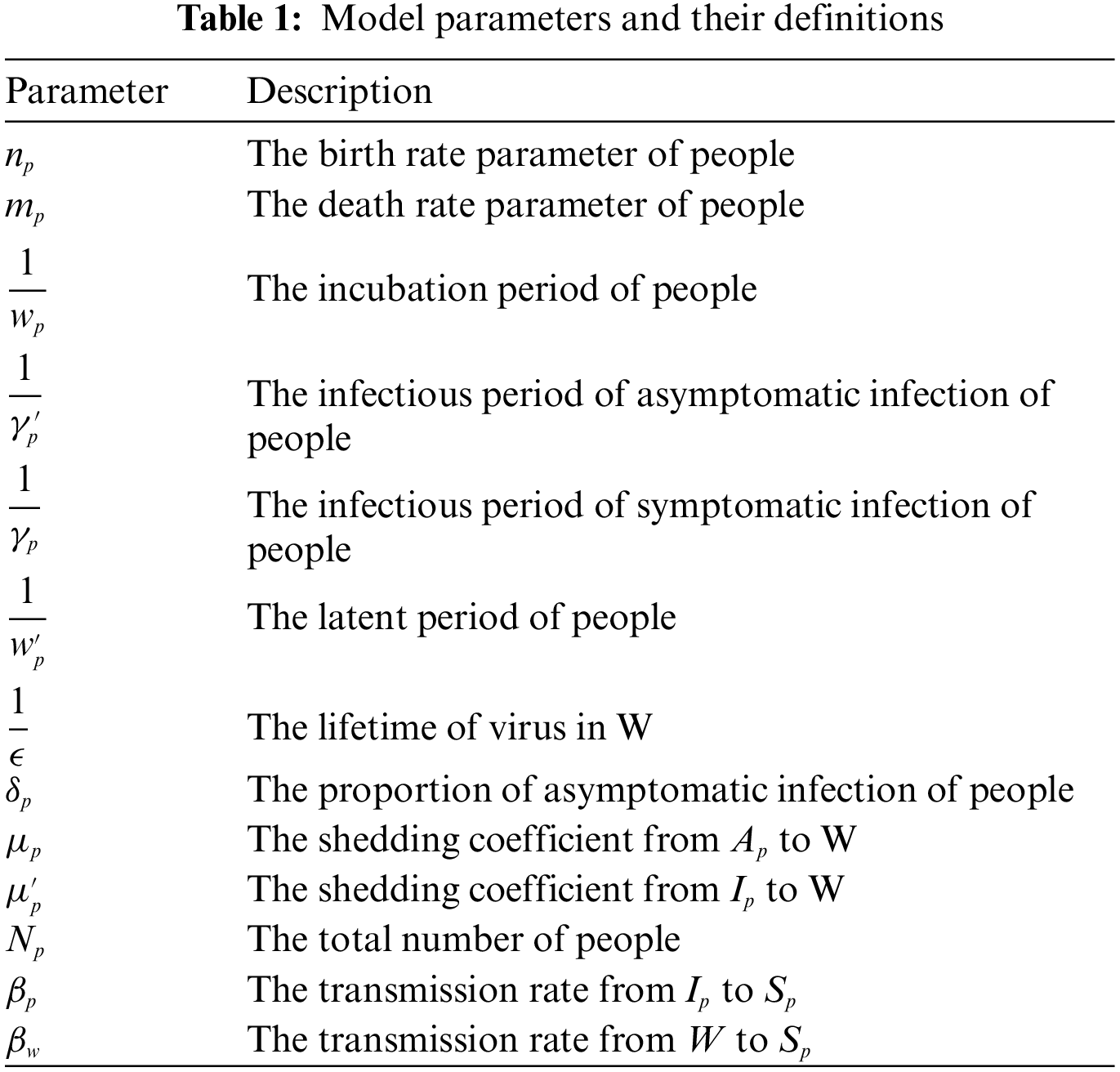
Figure 1: The model's flow diagram
In this paper, we assume
The process of normalization is implemented as follows [21]:
Therefore the six-dimensional integer-order COVID-19 model can be expressed by the following ordinary differential equation:
3.1 Implementation of Stochastic Description
We can provide an additional degree of realism by defining the white noise and Brownian motion and introducing a stochastic model. Therefore, we implement this idea by replacing random parameters
where
4 Dynamical Analysis of Solution
In this section, existence and uniqueness of the solution of the introduced model (2) and the equilibria of the system are presented.
4.1 Existence and Uniqueness of the Solution
Theorem 4.1. The coefficients of the stochastic differential Eq. (2) are locally Lipschitz.
Proof. We define the following kernel
Now we choose suitable a subset of
Then we continue our proof by applying:
So we define the path
where
Where
As a result, there is no global Lipschitz constant K valid on all
Lemma 4.1. Suppose that
Proof. The proof is presented in [40].
Therefore, we have local Lipschitz condition for the coefficient of
Theorem 4.2. For any given initial value
Proof. There exists a local solution on the interval
where
Let
Generalized Itô’s formula yields that
So we obtain
Therefore we obtain
where K is a positive constant and we have
Due to (7) and integrating both sides of (6) from to
Thus for every
where
So the statement
In this section, we establish sufficient conditions for the extinction of the disease. In order to form these conditions, we consider variation in the number of symptomatic infected people
In deterministic epidemiological models, basic reproduction number is planned to be a criterion of transmissibility of infectious agents. If
Lemma 4.2. Let Z(t):
Theorem 4.3. Let
Furthermore, if the assumptions
Proof. Itô’s formula yields that
So we obtain
where
According to Lemma 4.2, we obtain
where
Therefore
for
If
So we have
By dividing both sides of Eq. (10) by t such that
Letting
So we obtain
Letting
Therefore, our claim holds and this completes our proof.
Remark 4.1. Theorem 4.3 shows that the disease will decay exponentially to zero under suitable conditions. When the noises
Equilibria of the system can be estimated by setting the all derivatives equal to zero. This gives the system
In order to obtain the fixed points of COVID-19 model (2), we consider the solution of system (11) as follows
For
For
For
For
For
In order to achieve biologically relevant solutions, we find equilibrium points such that this system has positive solutions. There are two equilibrium points of system (11).
i) Disease free equilibrium point
ii) Endemic equilibrium point
In this section, we get deep insights into the model's dynamical behavior. For numerical simulation, the results of the implementation are given by the known Euler-Maruyama method [42]. We consider the following discretization model for
where
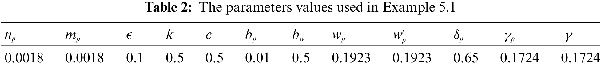
Example 5.1 In order to illustrate the adaptation and compatibility of the presented model with the deterministic model, we used the reported data in Wuhan City, China [21]. The parameters values used in the numerical simulation are given in Tab. 2.
The world health organization (WHO) reported an incubation period for COVID-19 between 2-10 days and the United States center for Disease Prevention and Control (CDC) estimates the incubation period for COVID-19 to be between 2-14 days. The mean incubation was 5.2 days (95% confidence interval CI: 4.1 to 7.0). According to the report of WHO on 3 March 2020, globally about 3.4% of reported COVID-19 cases have died. In this simulation, we assume that
In this example, if the intensities of the white noises of model (2) increase, the solution of model (2) will fluctuate around the disease free equilibrium. Fig. 3 shows the simulations with
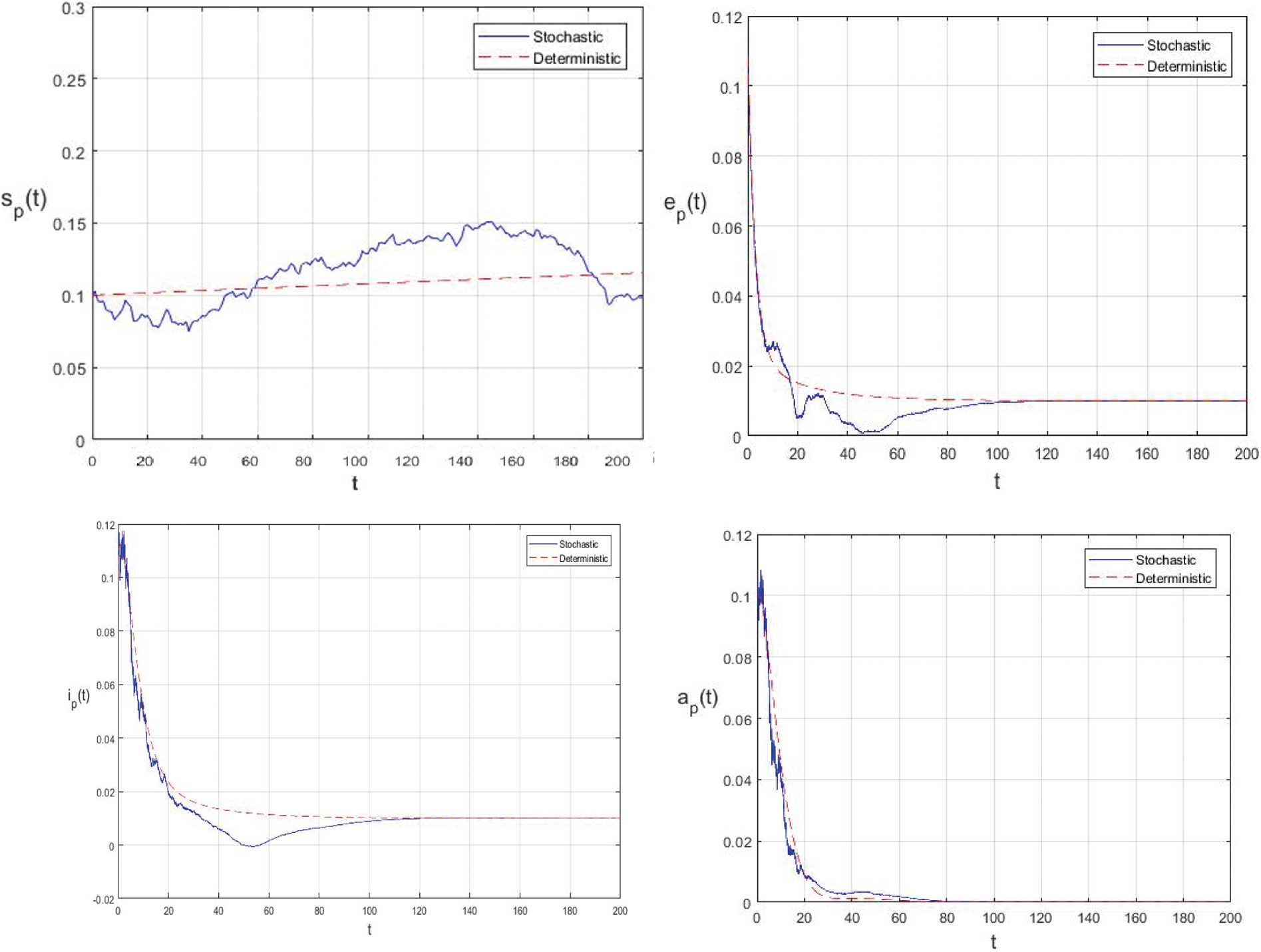
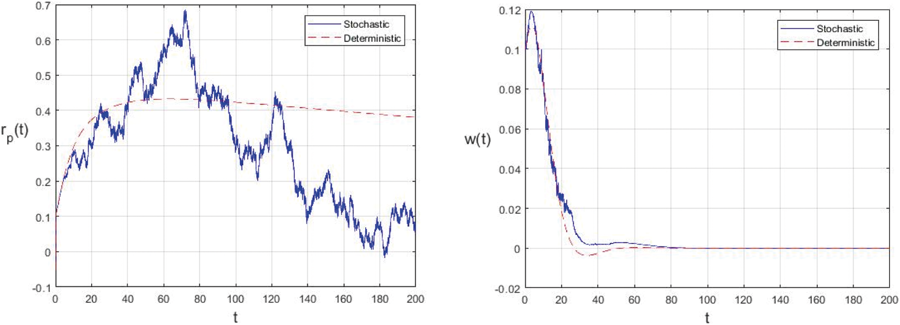
Figure 2: Comparison between the our presented stochastic model and deterministic model
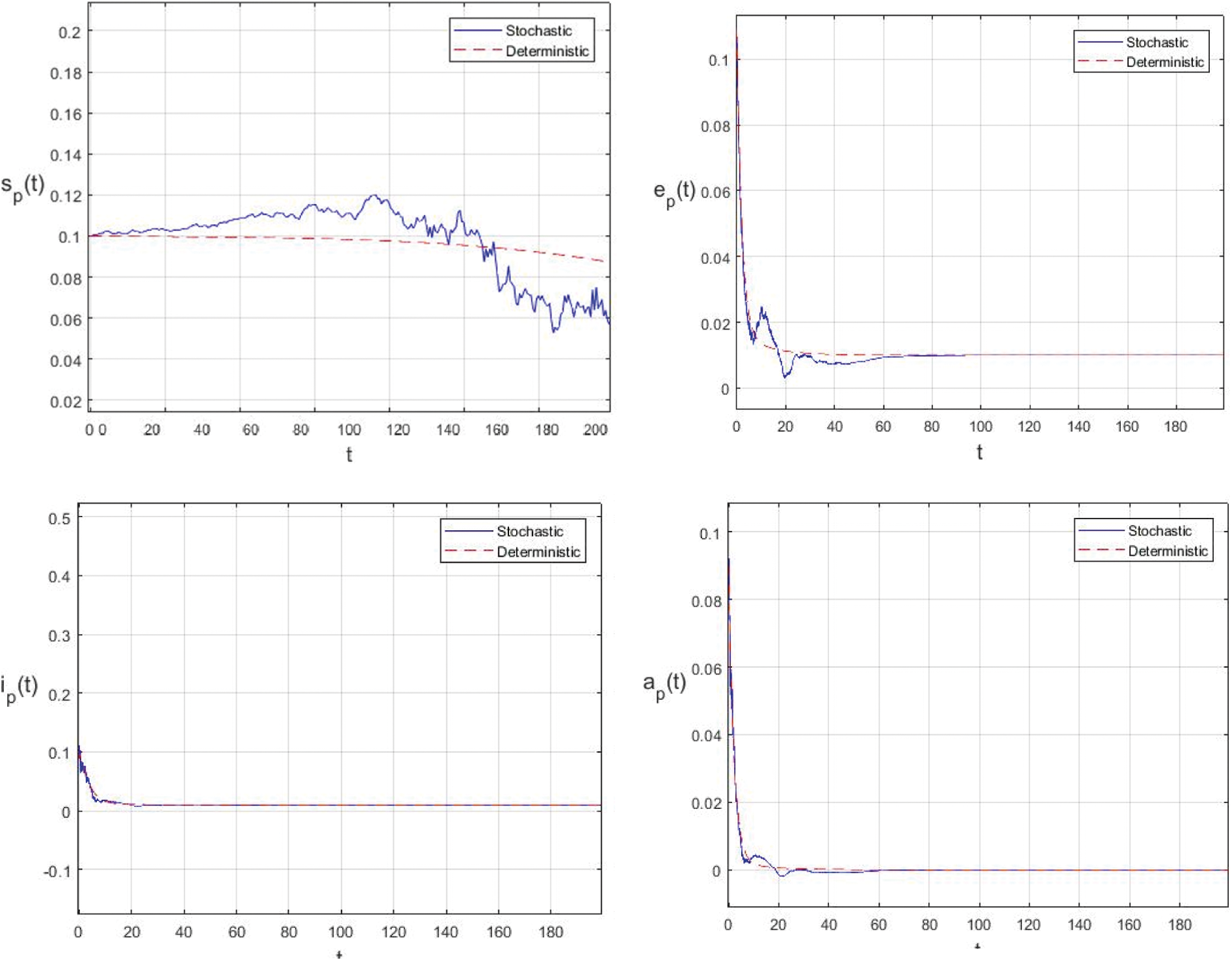
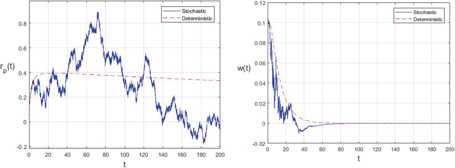
Figure 3: Comparison between the our presented stochastic model and deterministic model
Example 5.2 Since the information is changing and due to the lack of complete data on many parameters used in the proposed model, we now present some numerical simulations to illustrate the efficiency of our approach as an experiment for considering sensitivity analysis. Sensitivity analysis is commonly used to determine the robustness of model predictions to parameter values, since there are usually errors in collected data and assumptive parameter values. The parameter values used in this example are given in Tab. 3. In this example, we decrease the value of
Example 5.3 In this example we take the intensities of the white noises of the model (2) as
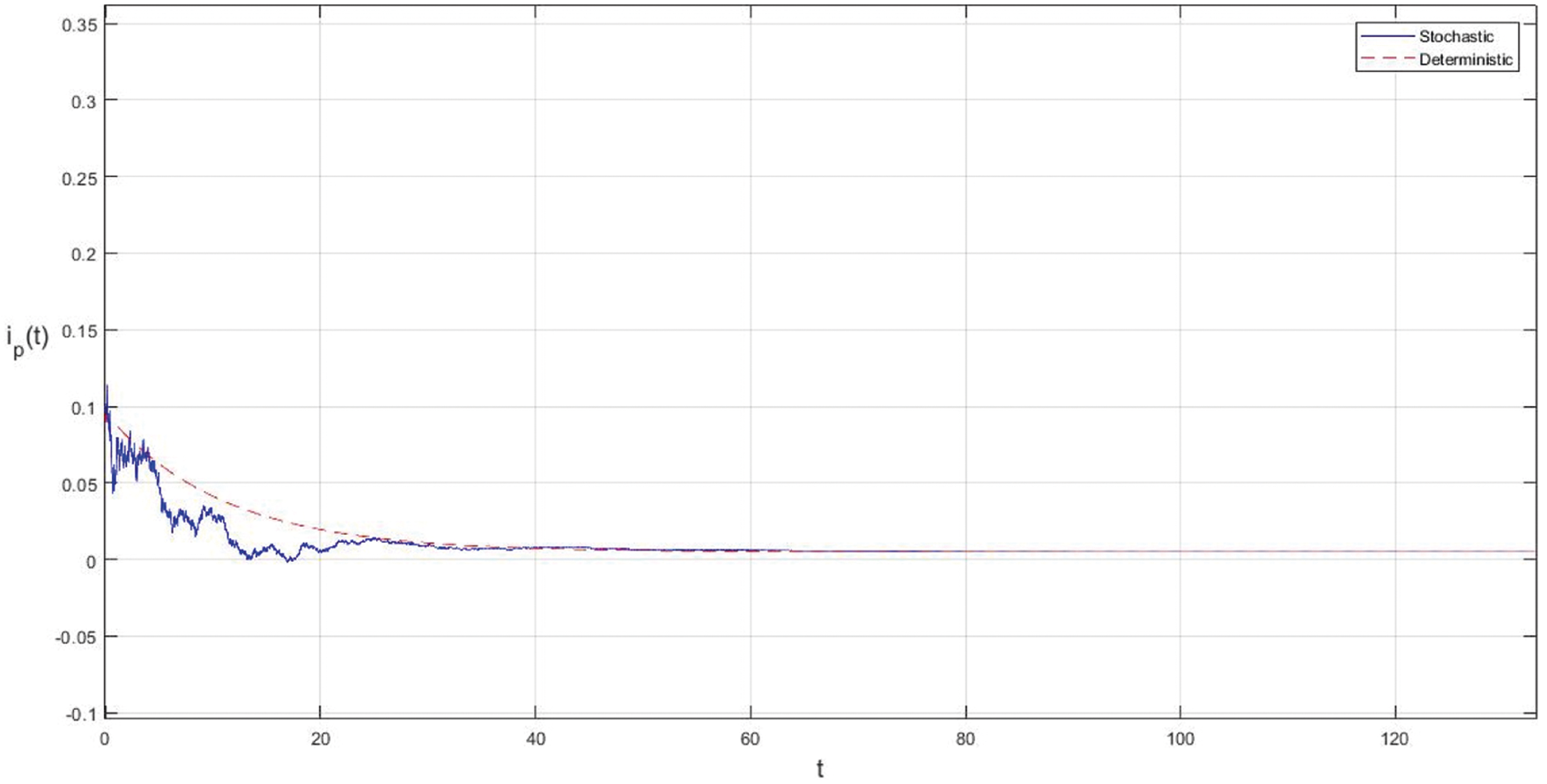
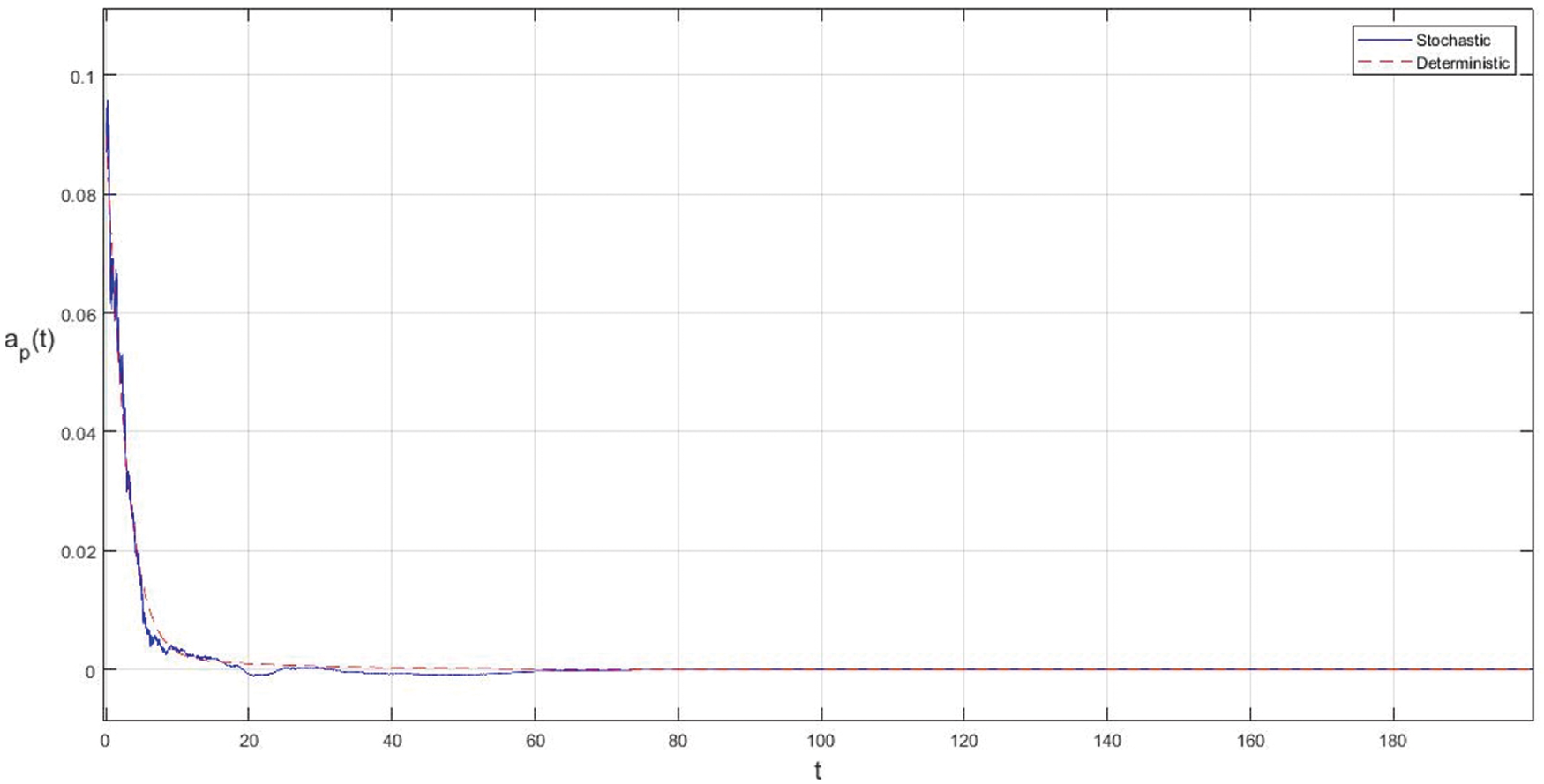
Figure 4: Effect of increasing the infectious period of symptomatic and asymptomatic infection of people
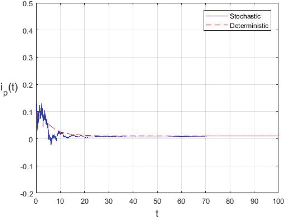
Figure 5: Extinction of the stochastic model under suitable conditions
In the proposed approach, the results have been obtained using the known Euler-Maruyama method as mentioned above. Moreover, to ensure the accuracy and precision of the obtained results, the comparison of the proposed scheme has been done with the deterministic model. In stochastic models, there are random variations due to uncertainties in the parameter. According to the presented comparisons (see Fig. 2 and Fig. 3), the results of our stochastic epidemic model are convergent to the deterministic model. The simulation results demonstrate the efficiency of our model, and the possibility of comparability of the stochastic model with the deterministic model. Evaluation results and dynamical analysis confirmed its effectiveness, efficiency, and user satisfaction. In this paper, we found that the infection can be controlled by suitable health decisions and herd immunity as a naturally occurring phenomenon can make the number of infectious cases descending. Furthermore, numerical simulation confirms the effect of high intensity white noises on the prevalence or extinction of the COVID-19. From the simulated findings (please see Fig. 4 and Fig. 5), it can be noticed that the our stochastic model shows a strong agreement with the deterministic case at different values of white noise. Additionally, graphical investigations confirmed that the infectious population tends to zero under suitable extinction conditions presented in Theorem 4.3. When the noises
In this paper, we have developed and analyzed an epidemic model for simulating transmissibility of the COVID-19 based on Reservoir-People transmission network. We construct a stochastic version of the Reservoir-People model by using the white noise and Brownian motion. Also, we proved that there is a unique solution for the presented stochastic model. Moreover, the equilibria of the system are considered. Also, we establish the extinction of the disease under some suitable conditions. Finally, the numerical simulation is carried out to demonstrate the efficiency of our model, and the possibility of comparability of the stochastic model with the deterministic model. Furthermore, numerical results demonstrate the validity of suitable conditions for the extinction of the disease. Since mathematical models are powerful tools to understand the dynamics of real world phenomena, particularly the transmission of an infectious disease, therefore this paper could lead to other studies that have included random and uncertainty of the model and can be more consistent with the reality of Coronavirus transmission. The presented results may be fruitful for the existing outbreak in a better way and can be used in taking defensive techniques to decrease the infection. The area of stochastic modeling has been extended recently, therefore this model is an indication for further study in this area. After getting high motivation from this paper and using ideas of modeling approaches in new researches (see [43–52]), hybrid stochastic fractional approach will be considered to investigate the dynamics of the COVID-19, as a scope of future works.
Funding Statement: The authors received no specific funding for this study.
Conflicts of Interest: The authors declare that they have no conflicts of interest to report regarding the present study.
1. H. W. Hethcote, “The mathematics of infectious diseases,” SIAM Review, vol. 42, no. 4, pp. 599–653, 2000. [Google Scholar]
2. N. Shahid, D. Baleanu, N. Ahmed, T. S. Shaikh, A. Raza et al., “Optimality of solution with numerical investigation for coronavirus epidemic model,” Computers Materials & Continua, vol. 67, no. 2, pp. 1713–1728, 2021. [Google Scholar]
3. D. Kramer, “Covid-19 pandemic modeling is fraught with uncertainties,” Physics Today, vol. 73, no. 6, pp. 25–27, 2020. [Google Scholar]
4. J. X. Yang, “The spreading of infectious diseases with recurrent mobility of community population,” Physica A: Statistical Mechanics and its Applications, vol. 541, Article ID 123316, 2020. [Google Scholar]
5. T. A. Yildiz and E. Karaoğlu, “Optimal control strategies for tuberculosis dynamics with exogenous reinfections in case of treatment at home and treatment in hospital,” Nonlinear Dynamics, vol. 97, no. 4, pp. 2643–2659, 2019. [Google Scholar]
6. M. S. Arif, A. Raza, M. Rafiq and M. Bibi, “A reliable numerical analysis for stochastic hepatitis B virus epidemic model with the migration effect,” Iranian Journal of Science and Technology, Transactions A, vol. 43, no. 5, pp. 2477–2492, 2019. [Google Scholar]
7. J. E. Macías-Díaz, N. Ahmed and M. Rafiq, “Analysis and nonstandard numerical design of a discrete three-dimensional hepatitis B epidemic model,” Mathematics, vol. 7, no. 12, Article ID 1157, 2019. [Google Scholar]
8. D. Baleanu, S. Sajjadi, A. Jajarmi, O. Defterli and J. H. Asad, “The fractional dynamics of a linear triatomic molecule,” Romanian Reports in Physics, vol. 73, no. 1, Article ID 105, 2021. [Google Scholar]
9. N. Ahmed, M. Jawaz, M. Rafiq, M. A. Rehman, M. Ali et al., “Numerical treatment of an epidemic model with spatial diffusion,” Journal of Applied Environmental and Biological Sciences, vol. 8, no. 6, pp. 17–29, 2018. [Google Scholar]
10. J. E. Macias-Diaz, A. Raza, N. Ahmed and M. Rafiq, “Analysis of a nonstandard computer method to simulate a nonlinear stochastic epidemiological model of coronavirus-like diseases,” Computer Methods and Programs in Biomedicine, vol. 204, Article ID 106054, 2021. [Google Scholar]
11. A. Raza, A. Ahmadian, M. Rafiq, S. Salahshour and M. Ferrara, “An analysis of a nonlinear susceptible-exposed-infected-quarantine-recovered pandemic model of a novel coronavirus with delay effect,” Results in Physics, vol. 21, Article ID 103771, 2021. [Google Scholar]
12. T. Sun and Y. Wang, “Modeling COVID-19 epidemic in heilongjiang province, China,” Chaos, Solitons & Fractals, vol. 138, Article ID 109949, 2020. [Google Scholar]
13. P. Melin, J. C. Monica, D. Sanchez and O. Castillo, “Analysis of spatial spread relationships of coronavirus (COVID-19) pandemic in the world using self-organizing maps,” Chaos, Solitons & Fractals, vol. 138, Article ID 109917, 2020. [Google Scholar]
14. A. Yousefpour, H. Jahanshahi and S. Bekiros, “Optimal policies for control of the novel coronavirus disease (COVID-19) outbreak,” Chaos, Solitons & Fractals, vol. 136, Article ID 109883, 2020. [Google Scholar]
15. B. Tang, X. Wang, Q. Li, N. L. Bragazzi, S. Tang et al., “Estimation of the transmission risk of the 2019-nCov and its implication for public health interventions,” Journal of Clinical Medicine, vol. 9, no. 2, Article ID 462, 2020. [Google Scholar]
16. P. Wu, X. Hao, E. H. Y. Lau, J. Y. Wong, K. S. M. Leung et al., “Real-time tentative assessment of the epidemiological characteristics of novel coronavirus infections in wuhan, China, as at 22 January 2020,” Eurosurveillance, vol. 25, no. 3, Article ID 2000044, 2020. [Google Scholar]
17. T. Sun and Y. Wang, “Modeling covid-19 epidemic in heilongjiang province, China,” Chaos, Solitons & Fractals, vol. 138, Article ID 109949, 2020. [Google Scholar]
18. D. Dansana, R. Kumar, A. Parida, R. Sharma, J. D. Adhikari et al., “Using susceptible-exposed-infectious-recovered model to forecast coronavirus outbreak,” Computers Materials & Continua, vol. 67, no. 2, pp. 1595–1612, 2021. [Google Scholar]
19. M. Naveed, M. Rafiq, A. Raza, N. Ahmed, I. Khan et al., “Mathematical analysis of novel coronavirus (2019-ncov) delay pandemic model,” Computers, Materials & Continua, vol. 64, no. 3, pp. 1401–1414, 2020. [Google Scholar]
20. M. Tahir, T. Shah, G. Zaman and T. Khan, “Stability behavior of mathematical model mERS corona virus spread in population,” Filomat, vol. 33, no. 12, pp. 3947–3960, 2019. [Google Scholar]
21. T. M. Chen, J. Rui, Q. P. Wang, Z. Y. Zhao, J. A. Cui et al., “A mathematical model for simulating the phase-based transmissibility of a novel coronavirus,” Infectious Diseases of Poverty, vol. 9, no. 1, pp. 1–8, 2020. [Google Scholar]
22. E. Hashemizadeh and M. Ebadi, “A numerical solution by alternative legendre polynomials on a model for novel coronavirus (covid-19),” Advances in Difference Equations, vol. 202, Article ID 527, 2020. [Google Scholar]
23. W. Gao, H. M. Baskonus and L. Shi, “New investigation of bats-hosts-reservoir-people coronavirus model and application to 2019-ncov system,” Advances in Difference Equations, vol. 2020, Article ID 391, 2020. [Google Scholar]
24. S. Cai, Y. Cai and X. Mao, “A stochastic differential equation sIS epidemic model with two correlated brownian motions,” Nonlinear Dynamics, vol. 97, pp. 2175–2187, 2019. [Google Scholar]
25. M. Fahimi, K. Nouri and L. Torkzadeh, “Chaos in a stochastic cancer model,” Physica A: Statistical Mechanics and its Applications, vol. 545, Article ID 123810, 2020. [Google Scholar]
26. H. Mehrjerdi, R. Hemmati and E. Farrokhi, “Nonlinear stochastic modeling for optimal dispatch of distributed energy resources in active distribution grids including reactive power,” Simulation Modelling Practice and Theory, vol. 94, pp. 1–13, 2019. [Google Scholar]
27. W. Shatanawi, A. Raza, M. S. Arif, K. Abodayeh, M. Rafiq et al., “An effective numerical method for the solution of a stochastic coronavirus (2019-ncovid) pandemic model,” Computers, Materials & Continua, vol. 66, no. 2, pp. 1121–1137, 2021. [Google Scholar]
28. W. Shatanawi, A. Raza, M. S. Arif, K. Abodayeh, M. Rafiq et al., “Design of nonstandard computational method for stochastic susceptible–infected–treated–recovered dynamics of coronavirus model,” Advances in Difference Equations, vol. 2020, Article ID 505, 2020. [Google Scholar]
29. J. Danane, K. Allali, Z. Hammouch and K. S. Nisar, “Mathematical analysis and simulation of a stochastic cOVID-19 levy jump model with isolation strategy,” Results in Physics, vol. 23, Article ID 103994, 2021. [Google Scholar]
30. K. Abodayeh, A. Raza, M. S. Arif, M. Rafiq, M. Bibi et al., “Stochastic numerical analysis for impact of heavy alcohol consumption on transmission dynamics of gonorrhoea epidemic,” Computers, Materials & Continua, vol. 62, no. 3, pp. 1125–1142, 2020. [Google Scholar]
31. A. Raza, M. Rafiq, D. Baleanu and M. S. Arif, “Numerical simulations for stochastic meme epidemic model,” Advances in Difference Equations, vol. 2020, Article ID 176, 2020. [Google Scholar]
32. W. Shatanawi, S. Arif, A. Raza, M. Rafiq, M. Bibi et al., “Structure-preserving dynamics of stochastic epidemic model with the saturated incidence rate,” Computers Materials & Continua, vol. 64, no. 2, pp. 797–811, 2020. [Google Scholar]
33. A. Raza, M. Rafiq, N. Ahmed, I. Khan, K. S. Nisar et al., “A structure preserving numerical method for solution of stochastic epidemic model of smoking dynamics,” Computers, Materials & Continua, vol. 65, no. 1, pp. 263–278, 2020. [Google Scholar]
34. M. A. Noor, A. Raza, M. S. Arif, M. Rafiq, K. S. Nisar et al., “Nonstandard computational analysis of the stochastic cOVID-19 pandemic model: An application of computational biology,” Alexandria Engineering Journal, vol. 61, no. 1, pp. 619–630, 2021. [Google Scholar]
35. K. Chatterjee, K. Chatterjee, A. Kumar and S. Shankar, “Healthcare impact of COVID-19 epidemic in India: A stochastic mathematical model,” Medical Journal Armed Forces India, vol. 76, pp. 147–155, 2020. [Google Scholar]
36. S. He, S. Tang and L. Rong, “A discrete stochastic model of the COVID-19 outbreak: Forecast and control,” Mathematical Biosciences and Engineering, vol. 17, pp. 2792–2804, 2020. [Google Scholar]
37. T., Rediat, “Stochastic modelling for predicting covid-19 prevalence in east Africa countries,” Infectious Disease Modelling, vol. 5, pp. 598–607, 2020. [Google Scholar]
38. X. Mao, Stochastic Differential Equations and Applications, Horwood Publishing, Chichester, 1997. [Google Scholar]
39. S. Cobzas, R. Miculescu and A. Nicolae, Stochastic Differential Equations and Applications, Springer International Publishing, Switzerland, 2019. [Google Scholar]
40. E. Pap, Handbook of Measure Theory, Amsterdam, North-Holland, 2002. [Google Scholar]
41. D. J. Higham, “An algorithmic introduction to numerical simulation of stochastic differential equations,” SIAM Review, vol. 43, no. 3, pp. 525–546, 2001. [Google Scholar]
42. B. Ivorra, M. R. Ferrández, M. Vela-Pérez and A. M. Ramos, “Mathematical modeling of the spread of the coronavirus disease 2019 (covid-19) taking into account the undetected infections. the case of China,” Communications in Nonlinear Science and Numerical Simulation, vol. 88, Article ID 105303, 2020. [Google Scholar]
43. D. Baleanu, S. Zibaei, M. Namjoo and A. Jajarmi, “A nonstandard finite difference scheme for the modeling and nonidentical synchronization of a novel fractional chaotic system,” Advances in Difference Equations, vol. 2021, Article ID 308, 2021. [Google Scholar]
44. D. Baleanu, S. Sajjadi, J. H. Asad, A. Jajarmi and E. Stiri, “Hyperchaotic behaviors, optimal control, and synchronization of a nonautonomous cardiac conduction system,” Advances in Difference Equations, vol. 2021, Article ID 157, 2021. [Google Scholar]
45. D. Baleanu, S. Sajjadi., A. Jajarmi and O. Defterli, “On a nonlinear dynamical system with both chaotic and nonchaotic behaviors: a new fractional analysis and control,” Advances in Difference Equations, vol. 2021, Article ID 234, 2021. [Google Scholar]
46. A. Jajarmi, D. Baleanu, K. Zarghami, K. Zarghami and S. Mobayen, “A general fractional formulation and tracking control for immunogenic tumor dynamics,” Mathematical Methods in the Applied Sciences, Inpress. [Google Scholar]
47. M. Fiza, A. Alsubie, H. Ullah, N. H. Hamadneh, S. Islam et al., “Three-dimensional rotating flow of MHD jeffrey fluid flow between two parallel plates with impact of hall current,” Mathematical Problems in Engineering, vol. 2021, Article ID 6626411, 2021. [Google Scholar]
48. H. Ullah, A. Alsubie, M. Fiza, N. H. Hamadneh, S. Islam et al., “Impact of hall current and nonlinear thermal radiation on jeffrey nanofluid flow in rotating frame,” Mathematical Problems in Engineering, vol. 2021, Article ID 9930017, 2021. [Google Scholar]
49. I. Khan, H. Ullah, M. Fiza, S. Islam, A. Z. Raja et al., “A levenberg-marquardt backpropagation method for unsteady squeezing flow of heat and mass transfer behaviour between parallel plates,” Advances in Mechanical Engineering, vol. 13, pp. 1–15, 2021. [Google Scholar]
50. A. Yazidi and H. L. Hammer, “Solving stochastic nonlinear resource allocation problems using continuous learning automata,” Applied Intelligence, vol. 48, no. 11, pp. 4392–4411, 2018. [Google Scholar]
51. H. Ullah, I. Khan, I. Khan, N. H. Hamadneh, M. F. Al-Asad et al., “Mhd boundary layer flow over a stretching sheet: A new stochastic method,” Mathematical Problems in Engineering, vol. 2021, Article ID 9924593, 2021. [Google Scholar]
52. I. Khan, H. Ullah, H. Alsalman, M. Fiza, S. Islam et al., “Falkner–Skan equation with heat transfer: A new stochastic numerical approach,” Mathematical Problems in Engineering, vol. 2021, Article ID 3921481, 2021. [Google Scholar]
 | This work is licensed under a Creative Commons Attribution 4.0 International License, which permits unrestricted use, distribution, and reproduction in any medium, provided the original work is properly cited. |