Computers, Materials & Continua DOI:10.32604/cmc.2022.024492
Article

Deep Learning and Machine Learning for Early Detection of Stroke and Haemorrhage

Zeyad Ghaleb Al-Mekhlafi1, Ebrahim Mohammed Senan2, Taha H. Rassem3, Badiea Abdulkarem Mohammed4,5,*, Nasrin M. Makbol5, Adwan Alownie Alanazi1, Tariq S. Almurayziq1 and Fuad A. Ghaleb6

1Department of Information and Computer Science, College of Computer Science and Engineering, University of Ha'il, Ha'il, 81481, Saudi Arabia
2Department of Computer Science & Information Technology, Dr. Babasaheb Ambedkar Marathwada University, Aurangabad, 431004, India
3Faculty of Science and Technology, Bournemouth University, Poole, BH12 5BB, UK
4Department of Computer Engineering, College of Computer Science and Engineering, University of Ha'il, Ha'il, 81481, Saudi Arabia
5College of Computer Science and Engineering, Hodeidah University, Hodeidah, 966, Yemen
6School of Computing, Faculty of Engineering, Universiti Teknologi Malaysia, Johor Bahru, Johor, 81310, Malaysia
*Corresponding Author: Badiea Abdulkarem Mohammed. Email: b.alshaibani@uoh.edu.sa
Received: 19 October 2021; Accepted: 24 December 2021

Abstract: Stroke and cerebral haemorrhage are the second leading causes of death in the world after ischaemic heart disease. In this work, a dataset containing medical, physiological and environmental tests for stroke was used to evaluate the efficacy of machine learning, deep learning and a hybrid technique between deep learning and machine learning on the Magnetic Resonance Imaging (MRI) dataset for cerebral haemorrhage. In the first dataset (medical records), two features, namely, diabetes and obesity, were created on the basis of the values of the corresponding features. The t-Distributed Stochastic Neighbour Embedding algorithm was applied to represent the high-dimensional dataset in a low-dimensional data space. Meanwhile,the Recursive Feature Elimination algorithm (RFE) was applied to rank the features according to priority and their correlation to the target feature and to remove the unimportant features. The features are fed into the various classification algorithms, namely, Support Vector Machine (SVM), K Nearest Neighbours (KNN), Decision Tree, Random Forest, and Multilayer Perceptron. All algorithms achieved superior results. The Random Forest algorithm achieved the best performance amongst the algorithms; it reached an overall accuracy of 99%. This algorithm classified stroke cases with Precision, Recall and F1 score of 98%, 100% and 99%, respectively. In the second dataset, the MRI image dataset was evaluated by using the AlexNet model and AlexNet + SVM hybrid technique. The hybrid model AlexNet + SVM performed is better than the AlexNet model; it reached accuracy, sensitivity, specificity and Area Under the Curve (AUC) of 99.9%, 100%, 99.80% and 99.86%, respectively.

Keywords: Stroke; cerebral haemorrhage; deep learning; machine learning; t-SNE and RFE algorithms

1  Introduction

The brain controls most of the body's activities, such as movement, speech, memory and cognition. It also regulates many other bodily systems’ functions. When the brain is healthy, it efficiently functions. However, when certain disorders develop in the brain, some of the consequences may result in death. One of these disorders is stroke or haemorrhagic stroke. When circulatory problems of the brain occur, resulting in malfunction and a stroke, the person is at risk of death or lifelong impairment for several years [1]. Stroke is considered the second leading cause of death in the world after ischaemic heart disease [2], although the main cause of stroke is unknown. Stroke is associated with abnormal metabolism, obesity, blood pressure, stress, etc. Stroke is divided into two types: ischaemic stroke called cerebral infarction and haemorrhagic stroke called cerebral haemorrhage. Ischaemic stroke is caused by cerebral vascular stenosis. Meanwhile, haemorrhagic stroke is caused by rupture of a cerebral blood vessel. The incidence of ischaemic stroke is higher than that of haemorrhagic stroke, and it represents 80%:20% of all stroke patients. Early and accurate diagnosis of both types of stroke is essential for patient survival. MRI and Computed Tomography (CT) scans are commonly used for early diagnosis of haemorrhagic stroke because of their non-invasive properties. Data mining methods are used based on a combination of medical examinations, environmental factors and family history to diagnose early ischaemic stroke. Electroencephalography (EEG) is also used to diagnose stroke due to its non-invasive properties and low cost. Medical experts examine and interpret the diagnosis of various physiological features of stroke through EEG, MRI or related medical examinations in manual diagnosis to predict stroke. However, manual diagnosis takes a long time and requires a large number of experts. Given the shortcomings of expert manual diagnosis, artificial intelligence techniques play a key role in medical diagnostics to reduce mortality, time and cost of medical errors. Many machine and deep learning algorithms rely on medical data and the features of each disease to improve disease prevention through early diagnosis and proper treatment [3]. Artificial intelligence techniques are a set of accurate and effective algorithms capable of modelling the complex and hidden relationships between many clinical examinations, extracting the engineering advantages and distinguishing all the engineering features of each disease from the other. In this research, we applied machine learning techniques to diagnose a medical record dataset that depends on a combination of medical examinations and environmental factors for early diagnosis of ischaemic stroke. Deep learning models have also been applied to the MRI dataset for the early diagnosis of haemorrhagic stroke. One of our main contributions is a hybrid between machine learning and deep learning techniques to diagnose the MRI dataset for the early diagnosis of haemorrhagic stroke.

Hung et al. [4] presented a dataset of electronic medical claim to compare the performance of Deep Neural Network (DNN) with machine learning algorithms for stroke diagnosis. DNN and Random Forest techniques have achieved high performance compared with the rest of the machine learning algorithms. Liu et al. [5] developed a hybrid machine learning approach for stroke prediction. Firstly, the missing values are determined by Radom Forest regression. Secondly, automated hyperparameter optimization based on DNN is carried out for stroke diagnosis. Thakur et al. [6] applied a feed forward neural network with back propagation to diagnose stroke by predicting cerebral ischaemia, which is one of the risk factors for stroke. Li et al. [7] presented a new method for diagnosing stroke through EEG signals. They worked on a multi-feature fusion by combining fuzzy entropy, wavelet packet energy and hierarchical theory. The results achieved by the fusion method showed superior results in the diagnosis of ischaemic and haemorrhagic stroke. Ong et al. [8] presented a comprehensive framework for determining the severity of ischaemic stroke from a radiographic text using machine learning and natural language processing. The natural language processing algorithm outperformed the other algorithms. Xie et al. [9] presented a CNN DenseNet model for stroke prediction based on the ECG dataset consisting of 12-leads. The system achieved a diagnostic accuracy of 99.99% during the training phase and an accuracy of 85.82% during the prediction phase. Cheon et al. [10] conducted a principal component analysis to extract the most important features from the medical records and feed the dataset to a deep learning network and five machine learning algorithms. The deep learning model achieved a higher accuracy than machine learning algorithms. Badriyah et al. [11] presented a system to diagnose a computerized tomography (CT) dataset. The CT images were processed, and all noise was removed. The Gray-Level Co-occurrence Matrix (GLCM) method was applied to extract the features. The hyperparameter of the dataset diagnostic process was tuned by using deep learning techniques. Phong et al. [12] presented three deep learning models, namely, GoogLeNet, LeNet and ResNet, for diagnosing brain haemorrhage; the aforementioned three models achieved accuracy rates of 98.2%, 99.7% and 99.2%, respectively. Gaidhani et al. [13] presented two deep learning models, namely, LeNet and SegNet, for MRI image diagnostics for stroke prediction. The SegNet model achieved a classification accuracy of 96% and a segmentation accuracy of 85%. Wang et al. [14] developed the Xception model for diagnosing a middle cerebral artery sign on CT images. The model achieved accuracy, sensitivity and specificity of 86.5%, 82.9% and 89.7%, respectively. Goyal et al. [15] used a heart disease dataset for the predictive analysis of stroke by deep learning technology. Sun et al. presented a method for treating functional electrical stimulation (FES) by using a finite state machine (FSM) which has been shown to be effective using additive data by accelerometer according to the calculated gain. The results proved that the calibration gain is close to 1 and the error rate is smaller compared to the error before calibration [16]. Venugopal et al. introduced a unique method for intracerebral haemorrhage (ICH) detection by extracting unique features called fusion-based feature extraction (FFE) with deep learning (DL) networks, this method is called FFEDL-ICH. The FFEDL-ICH method has four stages: preprocessing, segmentation, feature extraction, and classification. Firstly, the noise is removed and the images are enhanced with a Gaussian filter. Secondly, the lesion region was segmented by Fuzzy C-Means algorithm. Third, deep features were extracted by local binary patterns and residual network-152 methods. Finally, all features have been rated by DNN [17].

The main contributions of this research are as follows:

Firstly, for the first dataset (medical records):

•   Two features, namely, the diabetes feature based on the distinct values of glucose feature and the obesity feature based on the feature values of the BMI feature, are created.

•   The t-SNE algorithm is applied to represent the high-dimensional data in a low-dimensional space and the RFE algorithm to arrange the features and give each feature a percentage according to its priority and its correlation to the target feature.

Secondly, for the second dataset (MRI images):

•   Hybrid deep learning (AlexNet) and machine learning (SVM) is achieving high performance rather than the AlexNet model.

•   High-performance algorithms are generalized to assist clinicians in the early diagnosis of stroke and cerebral haemorrhage.

The rest of the paper is organized as follows: Section 2 describes an overview of stroke and deep and machine learning techniques. Section 3 deals with the processing of the two datasets. Section 4 describes the Classification techniques applied to the two datasets. Section 5 presents the experimental result analysis. Section 6 concludes the paper.

2  Overview

This section introduces the fundamentals of this research and is organized as follow:

2.1 Stroke Background

Cerebrovascular diseases are described as diseases of the brain that are affected either temporarily or permanently due to ischaemic causes (ischaemic stroke), haemorrhagic causes (haemorrhagic stroke) or congenital or acquired blood vessel damage. These diseases particularly affect the elderly or the middle-aged group. Ischaemic CVD is one of the causes of stroke; hence, early identification of CVD diseases by family members and consultation with specialists to receive proper treatment are essential to avoiding one of the causes of stroke. Initial assessment should include an evaluation of the airway and circulation. Cerebral haemorrhagic events are due to rupture of a cerebral vessel inside the parenchymal tissue and can occur as a result of a previous injury (tumour microangiopathy, hypertension or malformation). Stroke frequently suddenly occurs, with symptoms, such as headache, impaired consciousness, vomiting and focal neurological deficits determined by the site of cerebral haemorrhage. Once the specialist has been confirmed that the condition is stroke affecting a particular vascular area of the brain and causing a specific neurological deficit, the next step is to determine whether the cerebral haemorrhage exhibits an ischaemic or haemorrhagic nature. An MRI or CT scan technology is essential for this condition. In the event that the radiology confirms the presence of haemorrhagic stroke, the treatment consists of controlling the bleeding and reducing pressure with medications or a quick surgical intervention. The type of treatment depends on the location of the bleeding and whether the bleeding has occurred within or outside the brain tissue [18].

2.2 MRI

MRI (T1, T2 or FLAIR sequences) was not more effective than CT in the early detection of cerebral ischaemia or cerebral haemorrhage. However, MRI is more accurate and effective than CT in detecting the presence of certain infarcts and the site of cerebral haemorrhage and the causative mechanism; hence, MRI imaging can be recommended in the case of haemorrhagic stroke involving the vertebral region. In recent years, MRI has been standardized, allowing pathophysiological assessment of critical-stage stroke, and it is now the primarily neuroimaging modality in many specialty clinics for critical-stage stroke. MRI angiography is a non-invasive intracranial procedure. “Time-of-flight” (TOF) techniques, which do not give a clear contrast to the vein, are used for intracranial studies. Images of the brain are produced using the TOF technique to ensure that the signal from fixed tissues is minimized, and moving tissues (circulating blood) are distinguished. The MRI method achieved sensitivity and specificity of 100% and 95%, respectively, in the detection of intracranial vascular obstruction.

3  Materials and Methods

This section describes the methodology used to address the features of the two datasets: the first dataset consists of medical records of stroke, and the second dataset includes MRI images of cerebral haemorrhage. Fig. 1 illustrates the early diagnosis methodology for both first, stroke diagnosis, which used the medical records dataset and which underwent an enhancement process to replace missing values, remove outliers, and balance the dataset. New features were also created according to the values of existing features, the t-SNE algorithm was applied to represent the high-dimensional features in a low-dimensional space, the RFE algorithm was applied to extract the most important features that have a close and strong correlation with the target feature, and finally, the features were classified by SVM, KNN, Decision Tree, Random Forest and MLP classifiers. Second, regarding the diagnosis of cerebral haemorrhage, an MRI dataset was used. MRI images were enhanced by the average filter. The deep feature was extracted by the AlexNet model, then deep feature classification was done in two methods a) by fully connected layer and SoftMax function; b) by the hybrid method that uses SVM classifier to classify.

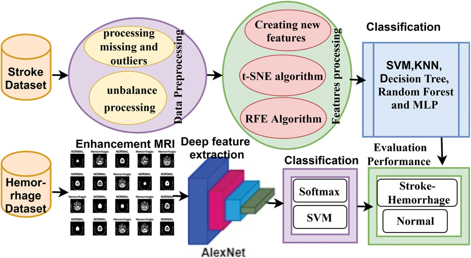
Figure 1: Methodology for classifying the stroke and cerebral haemorrhage datasets

3.1 Description of the Two Datasets

Two datasets were used in this study: Kaggle and MRI. The first dataset is based on medical and environmental tests (medical records). The second one is based on MRI of the brain for early detection of ischaemic and haemorrhagic strokes.

3.1.1 Description of Kaggle Dataset

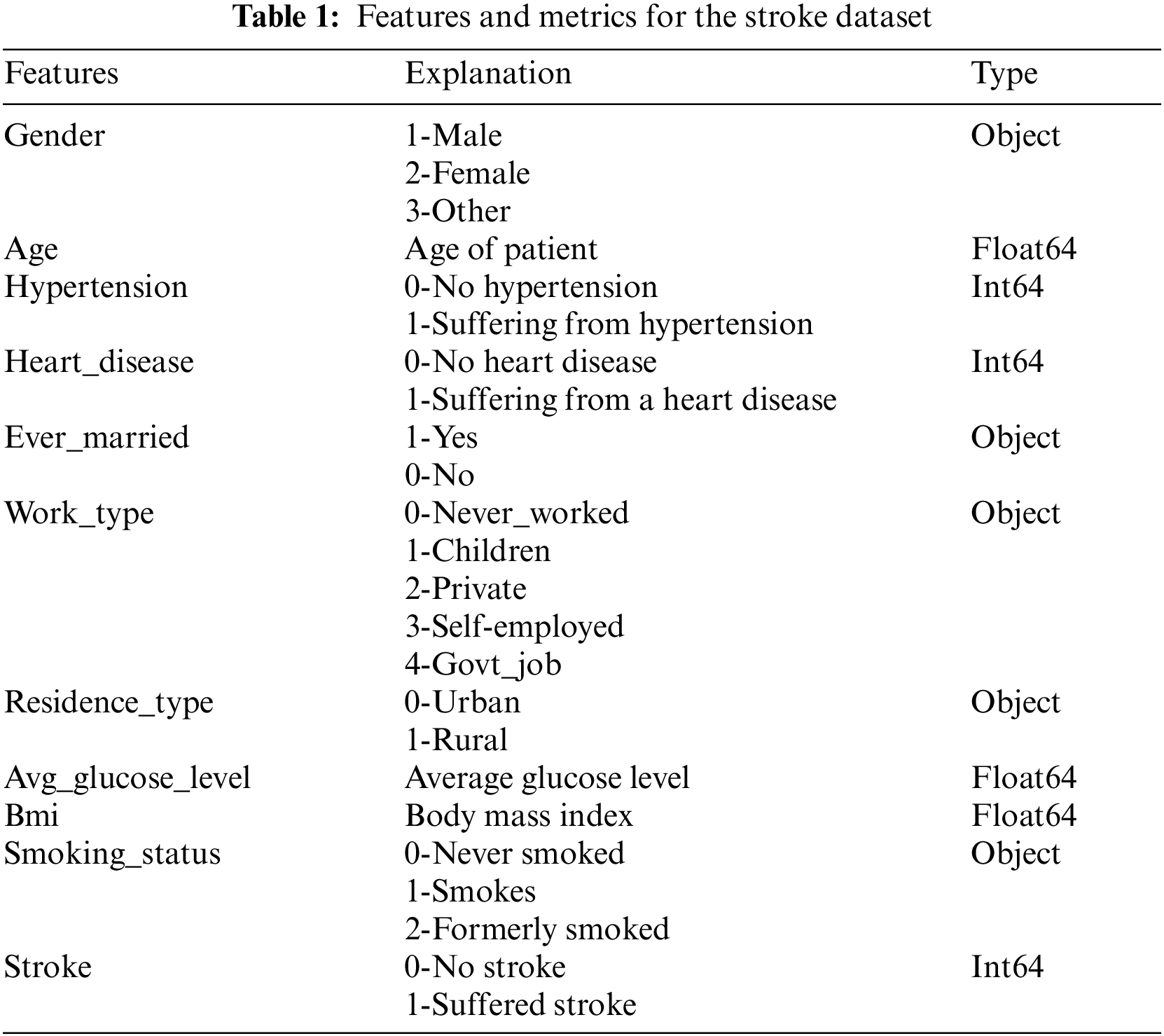
The first dataset, ‘Kaggle: HealthCare Problem: Prediction Stroke Patients’, includes some of the patient's medical records, such as hypertension, heart disease, physiological and environmental information. Tab. 1 illustrates the dataset, which contains 5110 rows, each row representing a patient, and 12 columns divided into 10 features, an identification column (ID) and a target feature column that is either stroke (1) or no stroke (0). Given that the dataset is unbalanced, with 4861 normal patients and 249 stroke patients, we will process it later during the training phase to find a data balance. This dataset is available at https://www.kaggle.com/fedesoriano/stroke-prediction-dataset.

3.1.2 Description MRI Dataset

The second dataset used in this study consists of normal and haemorrhagic brain MRI images collected from Near East Hospital, Cyprus [19]. The dataset contains 7032 images divided into 4343 normal images and 2689 cerebral haemorrhage images. All images were recorded in Digital Imaging and Communications in Medicine format, with a resolution of 512 × 512 pixels per image. Fig. 2 describes the brain images in the normal and haemorrhagic states. https://www.kaggle.com/abdulkader90/brain-ct-hemorrhage-dataset.

3.2 Pre-processing

Pre-processing is one of the most important steps in data mining and medical image processing. This step converts raw data into understandable information, removes noise, processes missing values and improves the image quality. In this study, the first dataset that contains medical images was improved by using optimization techniques in the field of data mining. Meanwhile, the second dataset that contains MRI images was enhanced by using optimization techniques in the field of medical image processing.

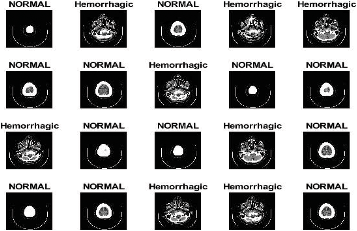
Figure 2: Brain images in normal and haemorrhagic states

3.2.1 Pre-processing of Kaggle Dataset

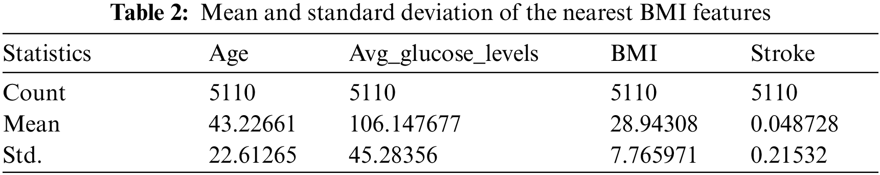
Data cleaning is one of the most important steps in data mining. This step involves removing outliers and replacing missing values. The dataset contains 201 missing BMI feature values, accounting for 3.93% of the total BMI feature values. The KNNImputer method was applied to predict the missing BMI values. The method was used to calculate the mean and standard deviation of the nearest five columns shown in Tab. 2. The dataset contains outliers, which are removed by outlier_function method. The outlier_function method calculated the interquartile range and first and third quartiles for each column in the dataset by computing the upper and lower limits. Approximately 166 outliers of the avg_glucose_level feature were removed, resulting in 166 rows being discarded. Then, the dataset has 4944 rows divided into 4717 normal (0) and 227 stroke (1) cases.

3.2.2 Pre-processing of the MRI Dataset

Some factors affect the quality of the MRI images, such as the patient's location inside the scanner, his movements and other factors that lead to a difference in the brightness of the MRI images. The difference in the MRI intensity value from black to white is called the bias field. Low, smooth or unwanted signals can destroy MRI images. Failure to correct the bias field will cause incorrect results in all processing algorithms. The preprocessing algorithms correct the failures caused by the bias field and remove the noise to obtain reliable accuracy in the following steps. Researchers were interested in pre-processing techniques for improving the image quality. In this work, the mean RGB colour was determined for MRI images, and the image was scaled for colour consistency. Finally, the MRI images were enhanced by using an average filter. All MRI images were resized in accordance with the deep learning models. Fig. 3 describes some MRI images after image enhancement.

Figure 3: MRI images after image enhancement

3.3 Dataset Unbalance Processing

Classification of the unbalanced dataset is one of the challenges due to the poor performance in the diagnosis because the evaluation measures require an equal distribution of the classes. In this study, the two datasets contain unbalanced classes. Therefore, we will address this imbalance.

3.3.1 Processing the Unbalance of Kaggle Dataset

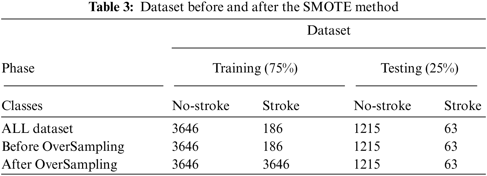
The first dataset (healthcare dataset) contains 5110 rows unbalanced. The dataset is unbalanced, and it is divided into 4861 no stroke (0) and 249 stroke (1) cases. The distribution rates of the dataset between no stroke and stroke cases are 95.1% and 4.9%, respectively. We can use the Spread SubSampling method, which is based on deleting many rows of no stroke cases. However, this method is not good for this dataset because the number of stroke cases is only 249; thus, we need to delete 4612 rows from the no stroke class. In this study, the Synthetic Minority Over-sampling Technique (SMOTE) method is used, which is a suitable method for finding a balance between the classes of the dataset. SMOTE randomly selects minority class rows, finds k nearest minority class neighbours and generates synthetic samples at a given point randomly for the minority class. Tab. 3 describes the dataset before and after the SMOTE method. The dataset is divided into 75% for training (3646 logs for class 0 and 186 logs for class 1) and 25% for testing (1215 logs for class 0 and 63 logs for class 1). Tab. 3 shows the preprocessing before and after the SMOTE method during the training phase, where the dataset for both classes is balanced, which has 3646 rows for normal and stroke.

3.3.2 Data Augmentation of the MRI Dataset

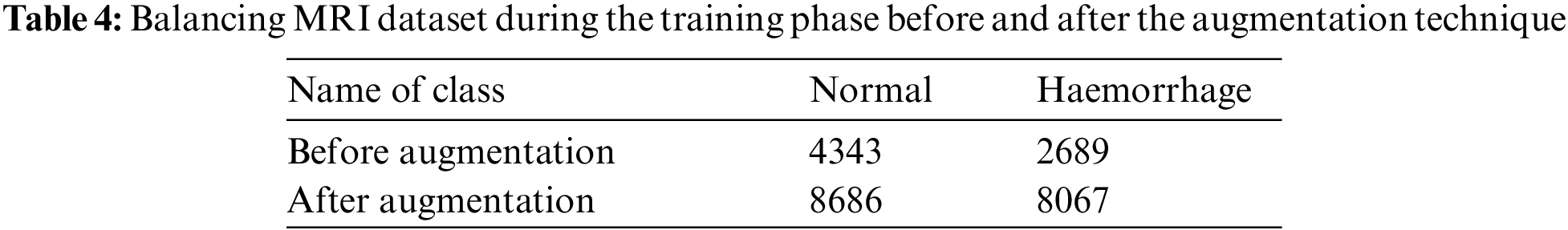
Deep learning techniques require a large dataset. However, the medical dataset lacks sufficient amounts of images; thus, more images solve this problem. Over training or overfitting when the dataset is small is one of the problems with deep learning. Data augmentation is a technique of augmenting data during the training phase by using random transformations to produce new images. In this study, the MRI dataset contains 7032 images divided into 4343 normal images and 2689 cerebral haemorrhage images. We notice the unbalance of the dataset; hence, the augmentation method is applied to find the balance in the dataset and increase the size of the dataset to solve the overfitting problem. The dataset is increased during the training phase by using the following operations: Rotation Shear, Zoom, Crop and Flip. Given that the cerebral haemorrhage class contains fewer images than the normal class, data augmentation operations are applied to the cerebral haemorrhage category more than the normal class. Tab. 4 describes the number of dataset images for each class before and after applying the data augmentation technique, where an increase in the size dataset and balance of the dataset are observed after applying the augmentation method.

3.4 Feature Engineering of the Kaggle Dataset

The features of Kaggle dataset were processed as follow:

3.4.1 Creating New Features

Creating new features is an important process that contributes to an effective diagnosis. This method is one of our contributions in this work, wherein two columns, namely, diabetes mellitus and obese, are created. The value of the features was calculated based on the value of the features in the columns ave-glucose-level and obese. The values of the added columns were filled in as follows:

•   If glucose > 126 is diabetes mellitus, then input one; otherwise, input zero.

•   If BMI > 30 is obese, then input one; otherwise, input zero.

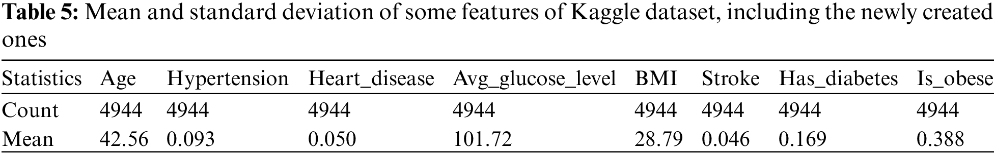
Thus, two important columns are created for the strike diagnosis. The dataset now contains 4944 rows and 14 features (columns). Tab. 5 describes the mean and standard deviation of the dataset for some features (columns), including the newly created features.

3.4.2 Recursive Feature Elimination (RFE) Algorithm

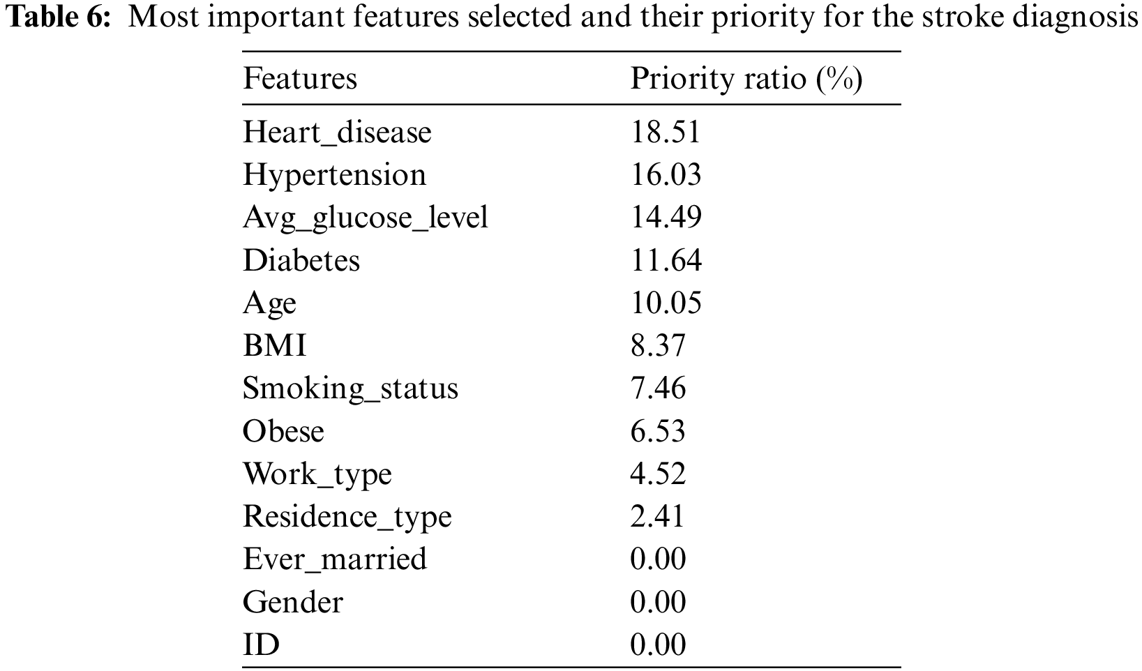
RFE is a widely used algorithm for selecting the features most closely correlated to the target feature in a classification or regression predictive model. This algorithm applies iterative processes to find and rank the best features and give a percentage for each feature in the target prediction process as follows. Firstly, a model that contains all the features in the dataset is created, and their importance is calculated. Secondly, the algorithm ranks the features in order of importance and removes the least important features on the basis of the RMSE model evaluation scale. The algorithm iterates until the preserved sub-feature is helpful in stroke diagnostic. Tab. 6 describes the most important features selected and ranked on the basis of their correlation to the target feature (labels); the table also indicates the percentage of participation of each feature for the stroke diagnosis [20].

3.4.3 t-Distributed Stochastic Neighbour Embedding (t-SNE) Algorithm

t-SNE is a modern nonlinear technique for scaling down a high dimensional dataset. The algorithm calculates the similar points in the high- and low-dimensional spaces. Conditional probability is used to calculate the similarity of points between the high and low dimensions based on the Gaussian probability density. The algorithm reduces the difference of conditional probabilities in high and low space to obtain ideal data in the low-dimensional space. Eq. (1) describes similar data points in the high-dimensional space. Meanwhile, Eq. (2) describes similar data points in the low-dimensional space through the t-SNE algorithm. The t-SNE algorithm reduces the Kullback–Leibler divergence through gradient descent to reduce the sum of conditional probability differences between the two high and low dimensional spaces. Eq. (3) describes the KL divergence to measure the divergence of the first conditional probability (high-dimensional data) from the second conditional probability (low-dimensional data).

P(Li /Lj )= S(Li , Lj )∑m≠iN⁡S(Li , Lm)(1)

Q(Hi /Hj )= S(Hi , Hj )∑m≠iN⁡S(Hi , Hm)(2)

KL=∑i⁡∑j⁡ P(Li , Lj )log P(Li /Lj ) Q(Hi , Hj )(3)

where L and H represent the data points in the high- and low-dimensional spaces, respectively.

3.5 Classification Techniques for Kaggle Dataset

The classification techniques used in this research with Kaggle dataset are as follow:

3.5.1 Support Vector Machine (SVM)

SVM works to solve classification problems for classes that are linearly separable or nonlinearly separable. The algorithm creates a hyperplane that separates the data into two classes. An ideal hyperplane is considered to have a maximum margin between classes. The data above the hyperplane belong to the first class, and the data below the hyperplane belongs to the second class [21]. When the data are non-separable due to their overlap, the solution is to transform the data from a nonlinear data space to a separable data space by finding the hyperlevel that causes the fewest possible errors.

3.5.2 K Nearest Neighbour (KNN)

This mechanism is called the lazy learning model because it is characterized by not mining data from knowledge. The algorithm trains and stores the training dataset for future use. When classifying a new condition (test point), the algorithm compares the test point with the stored data and finds the similarity between the test points and the stored dataset (training dataset). According to the principle of Euclidean distance, KNN measures the distance between the test data point and the stored data. Then, a new point is mapped to the nearest neighbour [22].

3.5.3 Neural Networks

This algorithm is called Multilayer Perceptron (MLP), and it is a family of neural networks, which means that it can achieve high accuracy provided that there is a sufficient number of data. A multi-layer perceiver consists of input layers for receiving images or text input, hidden layers for data processing and output layers for displaying the results. The model consists of at least one hidden layer [23]. The more hidden layers, the higher the computational cost; it may achieve better diagnostic results, but the excessive increase in the hidden layers is ineffective in terms of diagnostic accuracy. The algorithm reduces the error rate by comparing the predicted results with the actual results. The error rate is reduced by adjusting the weights in the backpropagation process. The process continues until the lowest error rate is obtained.

3.5.4 Decision Tree

A decision Tree is a machine learning algorithm called symbolic learning, wherein decision rules are closely related to trees and control the flow of operations. This algorithm consists of the root node (represents the entire dataset), the branch node (represents the features) and the root node (represents the final decision). In each decision, two or more branches are generated from each child node. The process continues until the process reaches the last decision, and there is no new decision (leaf node), meaning that each case depends on the values of the features involved in making a decision. Thus, the process starts from the root node and moves each state to the next branch until it reaches the leaf node [24]. The training dataset is divided into several subsets of data according to the selected feature values. The features remaining in each subset are evaluated, and logical decision rules are formulated to the next level of the tree.

3.5.5 Random Forest

Each tree learns with a random sample of data. The bootstrapping method iteratively and randomly replaces data in the same tree. Specifically, a decision is made every time the tree is trained on different data. Each tree has a different decision. Finally, the average of the predictions of all decision trees is taken. This method combines a large number of independent decision trees tested on random datasets with equal distribution.

3.6 Deep Learning and Hybrid for the MRI Dataset

The deep learning and hybrid methods that were used with MRI dataset are as follow:

3.6.1 Convolutional Neural Networks (CNNs)

CNNs are known as deep learning. The layers used by CNN are 2D; hence, they are suitable for image processing. The difference between CNN is that CNN weights are filters that are convoluted with the image to be processed [25]. In CNNs, each neuron receives connections from the previous layers and each other.

Fig. 4 shows the basic structure of the AlexNet model. The higher-level layers extract the most important deep features and define the classes of the input image. Each hidden layer increases the computational complexity of feature extraction. For example, the first layer can learn how to detect and select the edges of an image, the second layer learns to distinguish colours within an area of interest, the third layer learns to sense texture and so on. As shown in the previous figure, a convolutional network consists of the following types of layers:

•   Convolutional layer: the hidden layer where the tuning parameters and function of each cell and filters are specified. It is one of the most important main layers of CNN and works in a convolution fashion between the filter specified in a specified size with the image. The process is performed bypassing the filter in each part of the area of interest of the image.

•   Pooling layer: it is used to reduce the dimensions of the high-dimensional image to minimise the computational cost and the number of parameters and control excessive overfitting. The most common techniques are max pooling and average pooling.

•   Fully connected layer (FCL): It is the layer that works on classification and the core of the diagnostic stage. This layer is flat; hence, it requires an appropriate adaptation to transform the data into a vector for each image, as shown in the figure.

•   SoftMax layer: an activation function responsible for classification by marking each inputted image with its correct category.

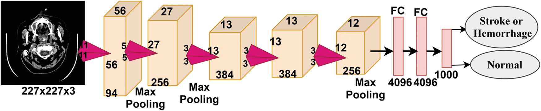
Figure 4: Basic structure of the AlexNet model

3.6.2 Transfer Learning: AlexNet

The transfer learning method is one of the techniques used in deep learning techniques. The idea is to take a network that has already been trained to solve related problems and is considered as a basic seed for solving new problems [26]. Pre-trained networks are distinguished by the fact that they have learned on millions of images to classify more than a thousand classes; hence, they have the ability to solve new problems. The AlexNet model, which is a pre-trained CNN, was selected in this study. The network contains 25 layers, the most important of which are five convolutional layers, three max pooling layers and three FCL layers [27].

The following steps represent the download of the AlexNet model:

1)    Create an image Datastore object to store images with their associated label.

2)    Divide the dataset into 80% for training and validation (80%:20%) and 20% for testing.

3)    Adapt the features of the inputted images based on the AlexNet model.

4)    Replace the last two layers of the AlexNet model: ‘fc8’ is fully connected.

5)    Carry out a model training in transfer learning while maintaining the weights of the first layers. The parameters to be configured are as follows:

6)    Classification of test images.

3.6.3 Hybrid Between AlexNet with SVM of the MRI Dataset

Another way to use AlexNet to effectively improve classification accuracy is to use the model to extract deep features from images and train the model [28]. This method is faster and easier to show the ability of deep neural networks to extract deep features because it does not need to iterate and go back to previous layers and only requires data to be passed once. The hybrid algorithm based on the AlexNet model and the SVM classifier consists of two separate blocks. The first is the extraction of deep features from the neural network itself using AlexNet, and the second is classification using the SVM classifier [29]. Therefore, the next steps will be to implement the hybrid technology and perform the following tasks from it [30,31]:

1)   Create an imageDatastore object to store images with their associated label.

2)   Divide the dataset into 80% for training and validation (80%:20%) and 20% for testing.

3)   Adapt the features of the inputted images based on the AlexNet model.

4)   Feature extraction: Each convolutional layer in the AlexNet model extracts deep features. For example, the first layer recognizes object boundaries, second layer extracts colour features, and another layer extracts complex shape features. Thus, each layer extracts deep features.

5)   Train the SVM classifier.

6)   Classify the test images.

4  Experimental Result and Discussion

The experiments and the findings of this research are as follow:

4.1 Splitting Dataset

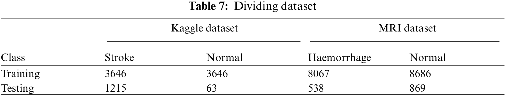
The first dataset consisted of 5110 instances divided into 4861 (95.1%) stroke patients and 249 (4.9%) normal instances. The imbalance of data during the training phase was addressed, and 4861 instances of stroke patients became normal. The dataset was divided into 75% for training and 25% for testing. The second dataset (MRI) consists of 7032 images divided into 4343 (61.76%) normal images and 2689 (38.24%) cerebral haemorrhage images. The imbalance of data during the training phase was addressed, and 8067 images became cerebral haemorrhage patients, and 8686 images are normal. The dataset was divided into 80% for training and validation (80%:20%) and 20% for testing. Tab. 7 describes the division of the two datasets after balancing during the training and selection phases for stroke and non-stroke patients for the first dataset and haemorrhage and normal patients for the MRI dataset.

4.2 Evaluation Metrics

The performance of machine learning algorithms on the stroke dataset (medical records) was evaluated using four statistical measures: Accuracy, Precision, Recall and F1 score. The MRI dataset was also evaluated by deep learning techniques (AlexNet) and hybrid techniques between deep learning and machine learning (AlexNet + SVM) using four statistical measures: Accuracy, Sensitivity, Specificity and AUC. The following equations describe how to calculate statistical measures. TP and TN represent correctly classified cases, whilst FP and FN represent incorrectly classified cases [32].

Accuracy=TN+TPTN+TP+FN+FP  *100%(4)

Precision=TPTP+FP  *100%(5)

Recall =TPTP+FN*100%(6)

F1score=2 * Precision * Recall Precision+Recall ∗100(7)

Sensitivity=TPTP+FN  *100%(8)

Specificity=TNTN+FP∗100(9)

AUC =True Positive RateFalse Positive Rate=SensitivitySpecificity(10)

where:

TP: denotes the patients’ cases (stroke or haemorrhage) that have been correctly classified.

TN: represents normal patients that are correctly classified. FN: indicates the patients’ cases (stroke or haemorrhage) classified as normal.

FP: represents the normal conditions classified as (stroke or haemorrhage).

4.3 Results of Kaggle Dataset

Two features, namely, diabetes and obese, were created after the dataset was balanced. The t-SNE algorithm was applied to represent the high-dimensional data in the low-dimensional data space. The RFE algorithm was applied to rank the features according to their priority and their relation to the target feature. The features ranked in order of priority were fed to the SVM, KNN, Decision Tree, Random Forest and MLP classifiers. All classifiers achieved promising results in the early diagnosis of stroke. The loss function has been reduced to neutralize the behaviour of classification algorithms by adjusting the hyper-parameter. Tab. 8 describes the results achieved by the classification algorithms for diagnosing normal and stroke cases. We display the results of the stroke case diagnosis. The Random Forest algorithm is superior to the rest of the algorithms because it achieved an overall accuracy of 99% and Precision, Recall and F1 score of 97%, 100% and 98%, respectively. The MLP algorithm achieved an overall accuracy of 98% and Precision, Recall and F1 score of 100%, 95% and 98%, respectively. Decision Tree algorithm achieved an overall accuracy of 98% and Precision, Recall and F1 score of 98%, 100% and 99%, respectively. Meanwhile, the two algorithms, namely, SVM and KNN, achieved an equal overall accuracy of 96%. Meanwhile, SVM achieved Precision, Recall and F1 score of 92%, 100% and 96%, respectively.

4.4 Results of the MRI Dataset

The findings from using MRI dataset are as follow:

4.4.1 Results of MRI Dataset by Using the CNN AlexNet Model

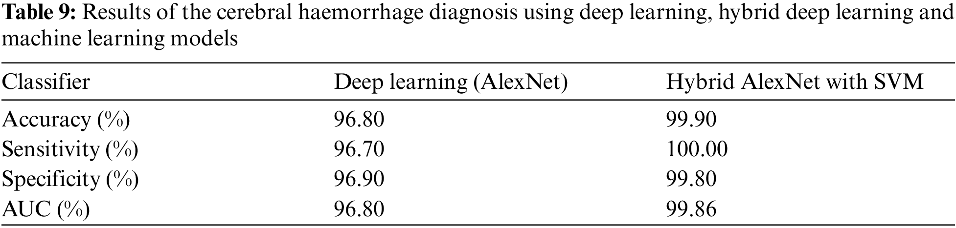
The MRI dataset was balanced by using data augmentation technique [33]. The weights and parameters of the AlexNet model are set as follows: The optimizer is Adam, the learning rate is 0.0001, the mini batch size is 120, the max epoch is 10, the validation frequency is 50, the training time is 128 min and 16 s, and the execution environment is GPU. An experiment was conducted by the AlexNet model to evaluate the MRI dataset. The model achieved optimal results for the diagnosis of cerebral haemorrhage. Fig. 5 describes the confusion matrix for cerebral haemorrhage diagnosis. Tab. 9 describes the interpretation of the confusion matrix where the model achieved accuracy, sensitivity, specificity and AUC of 96.8%, 96.70%, 96.90% and 96.80%, respectively. The confusion matrix describes samples correctly and incorrectly classified, where 520 images of cerebral haemorrhage were correctly classified (TP = 96.7%), and 18 images of cerebral haemorrhages were classified as normal (FP = 1.3%). Meanwhile, 842 images of normal were correctly classified (TN = 96.9%), and 27 images of normal were classified as cerebral haemorrhage (FN = 1.9%).

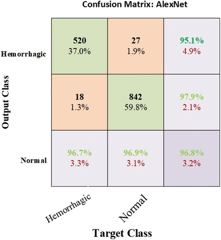
Figure 5: Confusion matrix for cerebral haemorrhage diagnosis by CNN AlexNet model

4.4.2 Results of the MRI Dataset by Hybrid AlexNet with SVM

Data augmentation technique is implemented to balance the dataset and overcome the problem of overfitting [34]. The use of deep learning techniques requires high-performance computers and takes a long time. Accordingly, the hybrid techniques between deep learning and machine learning are used to solve these problems and achieve better results than using deep learning models. This experiment is one of our main contributions in this research. This hybrid algorithm works as follows: The images are optimized using average filter. AlexNet model is applied to extract deep features. Then, the last three classification layers are removed from AlexNet model and replaced by SVM machine learning algorithm. Accordingly, we made a hybrid between deep and machine learning techniques. Fig. 6 describes the confusion matrix for cerebral haemorrhage diagnosis. Tab. 9 describes the interpretation of the confusion matrix where the model achieved accuracy, sensitivity, specificity and AUC of 99.9%, 100%, 99.80% and 99.86%, respectively. The confusion matrix describes samples correctly and incorrectly classified. The images of cerebral haemorrhage were correctly classified with a percentage of TP = 100%, while 867 images were correctly classified with a percentage of TN = 99.8%. Two images of the normal case were classified as cerebral haemorrhage with a percentage of FN = 0.1%. Thus, the hybrid method using deep learning and machine learning (AlexNet + SVM) is superior to AlexNet deep learning.

Figure 6: Confusion matrix for the cerebral haemorrhage diagnosis by hybrid AlexNet + SVM

5  Discussion and Comparison with Related Studies

Pattern recognition of MRI images and medical records are important in the early diagnosis of stroke and cerebral haemorrhage. Due to the shortcoming of manual diagnosis by experts, artificial intelligence techniques are used for an accurate and reliable diagnosis. In this study, machine learning techniques were evaluated on a medical records dataset, and the performance of deep learning techniques was evaluated on the MRI dataset, in addition to the use of a modern hybrid technique between deep learning (AlexNet) and machine learning (SVM). First, due to the optimization of the medical records dataset and feature processing by the RFE and t-SNE algorithms, all machine learning classifiers achieved superior results. Second, for the MRI dataset that has been optimized, removed all noise, and extracted the deep representative features by the AlexNet model, it has achieved superior results. Third, through the hybrid technique that consists of two blocks: the first, deep learning block is AlexNet to extract deep features, and the second block is SVM machine learning technique that used to classify the features extracted from the first block. This hybrid technique achieved the best results compared to the previous technologies. Tab. 10 and Fig. 7 describe a comparison of the results of the proposed systems for evaluating the medical records dataset and MRI with the current relevant systems. Where it is noted that our proposed systems are superior to all related systems. The systems of the previous studies reached an accuracy of between 83.34% and 96.56%, while our systems reached an accuracy of 99%, 96.8% and 99.9% for the random forest classifier, AlexNet network, and AlexNet + SVM, respectively. While the previous studies’ systems achieved a sensitivity of between 64.32% and 95.65%, while our systems reached a sensitivity of 100%, 96.70%, and 100% for the random forest classifier, AlexNet network, and AlexNet + SVM, respectively. As for the specificity, the previous studies’ systems achieved a specificity of between 83.56% and 97.93%, while our systems reached a specificity of 96.9% and 99.8% for AlexNet and AlexNet + SVM, respectively.

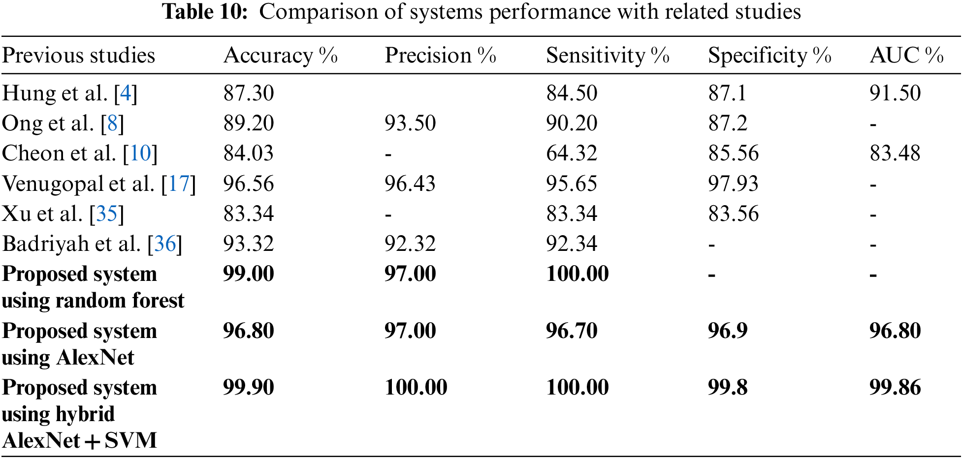
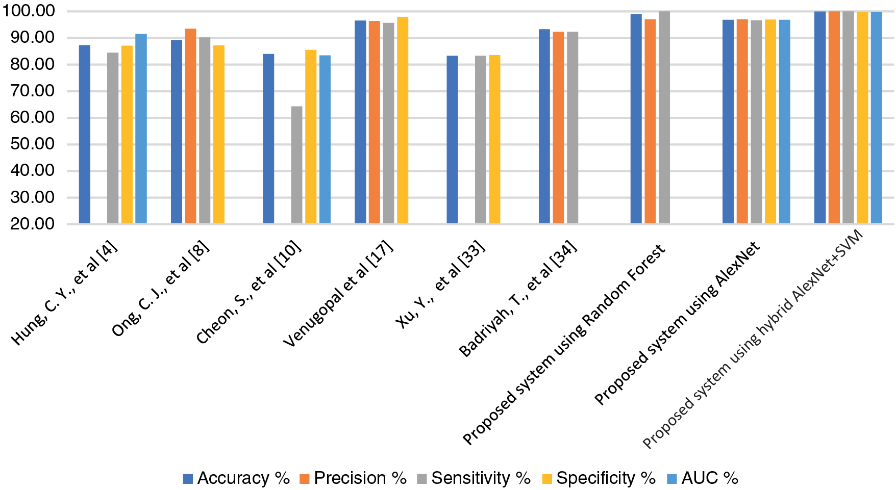
Figure 7: Display a comparison of the proposed systems with previous relevant studies

6  Conclusion

The brain controls most of the body's functions. The brain may suffer from some disorders that lead to permanent disability or death. Stroke and cerebral haemorrhage are amongst the types of brain disorders. Machine learning and deep learning techniques have played a key role in the early diagnosis of stroke and cerebral haemorrhage due to the limitations of manual diagnosis by physicians and experts. In this work, we used two datasets. The first dataset is a medical record of medical examinations and environmental and physiological changes. The SMOTE method was applied to balance the dataset, and the missing values were replaced by using the KNNImputer method, and outliers were removed. Two features, namely, diabetes and obese, were created based on the values of the corresponding features. The high-dimensional data was represented in a low-dimensional space by the t-SNE algorithm. Then, the features were arranged according to their priority and their correlation to the target feature by the RFE algorithm. Finally, these features were fed to five machine learning algorithms, namely, SVM, KNN, Decision Tree, Random forest and MLP. The dataset was divided into 75% for training and 25% for testing. All algorithms achieved superior results. The random forest algorithm achieved the best result, achieving an overall accuracy of 99% and Precision, Recall and F1 score of 98%, 100% and 99%, respectively. The second dataset consists of MRI images. All images have undergone an optimization process to remove noise by the average filter. A data augmentation technique has also been applied to balance the dataset and avoid overfitting. The dataset was divided into 80% for training and validation (80%:20%) and 20% for testing. The deep features were extracted by the AlexNet model, where 9216 features were extracted for each image and stored in a 1D vector. Then, the features were classified by using the deep learning (AlexNet) model and machine learning (SVM). The hybrid algorithm between machine learning and deep learning achieved better results than the deep learning model (AlexNet). AlexNet + SVM achieve accuracy, sensitivity, specificity and AUC of 99.9%, 100%, 99.80% and 99.86%, respectively.

Acknowledgement: We would like to acknowledge the Scientific Research Deanship at the University of Ha'il, Saudi Arabia, for funding this research.

Funding Statement: This research has been funded by the Scientific Research Deanship at the University of Ha'il, Saudi Arabia, through Project Number RG-20149.

Conflicts of Interest: The authors declare that they have no conflicts of interest to report regarding the present study.

This work is licensed under a Creative Commons Attribution 4.0 International License, which permits unrestricted use, distribution, and reproduction in any medium, provided the original work is properly cited.