DOI:10.32604/cmc.2022.024576
| Computers, Materials & Continua DOI:10.32604/cmc.2022.024576 | |
| Article |
Short-Term Wind Energy Forecasting Using Deep Learning-Based Predictive Analytics
1Department of Electrical Power Engineering & Mechatronics, Tallinn University of Technology, Tallinn, 19086, Estonia
2Department of Electrical and Computer Engineering, COMSATS University Islamabad (Lahore Campus), 54000, Pakistan
3Department of Electrical Engineering, Government College University, Lahore, 54000, Pakistan
4Department of Computer Science, COMSATS University Islamabad, Islamabad, 45550, Pakistan
5Department of Information and Communication Engineering, Yeungnam University, Gyeongsan, 38541, Korea
*Corresponding Author: Jin-Ghoo Choi. Email: jchoi@yu.ac.kr
Received: 22 October 2021; Accepted: 10 December 2021
Abstract: Wind energy is featured by instability due to a number of factors, such as weather, season, time of the day, climatic area and so on. Furthermore, instability in the generation of wind energy brings new challenges to electric power grids, such as reliability, flexibility, and power quality. This transition requires a plethora of advanced techniques for accurate forecasting of wind energy. In this context, wind energy forecasting is closely tied to machine learning (ML) and deep learning (DL) as emerging technologies to create an intelligent energy management paradigm. This article attempts to address the short-term wind energy forecasting problem in Estonia using a historical wind energy generation data set. Moreover, we taxonomically delve into the state-of-the-art ML and DL algorithms for wind energy forecasting and implement different trending ML and DL algorithms for the day-ahead forecast. For the selection of model parameters, a detailed exploratory data analysis is conducted. All models are trained on a real-time Estonian wind energy generation dataset for the first time with a frequency of 1 h. The main objective of the study is to foster an efficient forecasting technique for Estonia. The comparative analysis of the results indicates that Support Vector Machine (SVM), Non-linear Autoregressive Neural Networks (NAR), and Recurrent Neural Network-Long-Term Short-Term Memory (RNN-LSTM) are respectively 10%, 25%, and 32% more efficient compared to TSO's forecasting algorithm. Therefore, RNN-LSTM is the best-suited and computationally effective DL method for wind energy forecasting in Estonia and will serve as a futuristic solution.
Keywords: Wind energy production; energy forecast; machine learning
The worldwide energy demand is increasing with every passing year so is the environmental pollution due to the brown energy generation from fossil fuels. Therefore, the uses of Renewable Energy Resources (RES) like solar and wind have gained popularity due to lower carbon emissions. However, wind energy generation is variable and unstable due to variations in wind speed [1,2]. The variable nature of wind depends on geographical area, weather, time of day, and season. Therefore, predicting wind power generation with 100% accuracy is a very difficult task [3]. However, this prediction is highly important for the management of demand and supply in power grids and also has an economic impact [4,5]. This prediction was usually made using statistical methods [6], such as moving average and autoregressive, but the accuracy of the models was relatively low. Machine learning (ML) based forecasting algorithms are a widely used tool due to their property to capture nonlinearities in the data with high accuracy, but machine learning algorithms usually require a large dataset of formation to develop an efficient forecasting model. These models are trained, validated, and tested; sometimes they still require retraining to obtain more precise results [7]. The forecasting models are usually divided into three categories, such as short-term forecasting (few minutes to 24 h), medium-term forecasting (days-ahead to week-ahead), and long-term forecasting (month-ahead to year-ahead) [8]. In this study, the real-time dataset of Estonian wind energy generation is used [9,10] for the development of these forecasting models.
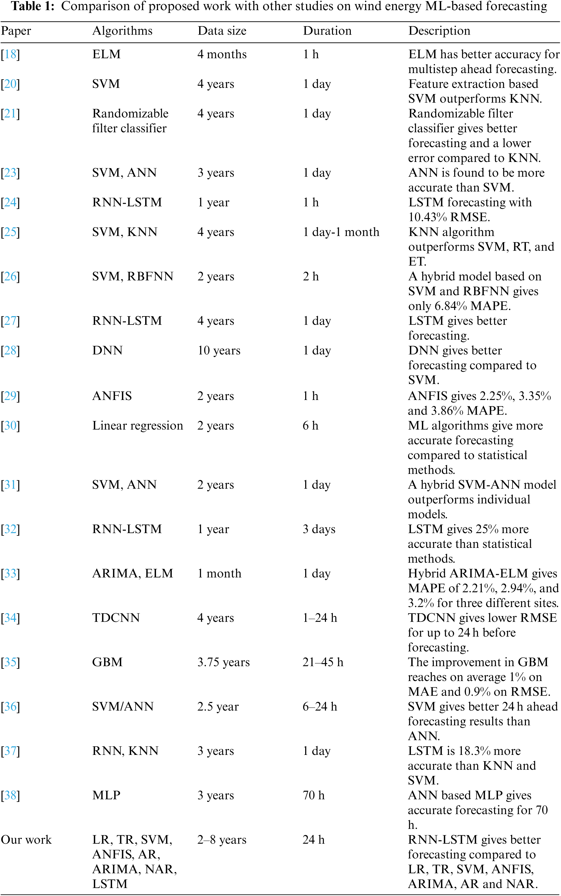
In the past, several research works have been developed using deep methods for wind speed forecasting and wind power generation forecasting. A bibliometric visualization of the keywords used in previous studies conducted in the past 5 years related to wind energy furcating has been made in VOS viewer software and depicted in Fig. 1. The figure shows the keywords used in 238 articles in the last five years related to wind energy forecasting. The forecasting of the wind speed in a university campus in Switzerland is being made using the ridge regression technique [11]. In a similar study [12], different ML algorithms like Support Vector Machine (SVM), K-Nearest Neighbor (KNN) regression, and random forest are compared for the forecasting of wind speed and corresponding energy generation for the day-ahead prediction horizon. A hybrid genetic algorithm and SVM-based algorithm are developed and tested for under-learning and overlearning scenarios of forecasting to determine the optimal solution [13]. A review of a supervised ML algorithm is made in [14]. In another work, ANN-based algorithms are developed and simulated to predict wind energy generation for grid stability [15]. A novel Cartesian genetic Artificial Neural Network (ANN) based algorithm is also proposed for wind energy forecasting in [16], which includes Hybrid regression based on SVM, Convolutional neural network (CNN), and singular spectrum analysis (SSA). The experimental results showed that SVM gave better predictions [17]. In [18], Extreme Machine Learning (ELM) algorithms have been used to forecast the wind speed for energy generation. A comparison of ELM, Recurrent Neural Networks (RNN), CNN, and fuzzy models is also given in [19–22] and future research directions are also explored. Tab. 1 provides a summary and comparison of the few known research articles related to wind energy forecasting using ML algorithms including Self-adaptive Evolutionary Extreme Learning Machine (SAEELM), Multilayer Perceptron (MLP), Random Forest (RF), Linear Regression (LR), Extremely Randomized Trees (ET), Radial Basis Function Neural Network (RBFNN), Gradient Boosting Algorithm (GBM), Tree Regression (TR), Long Short-Term Memory Networks (LSTM), Two-stream Deep Convolutional Neural Networks (TDCNN), Mean absolute percentage error (MAPE).
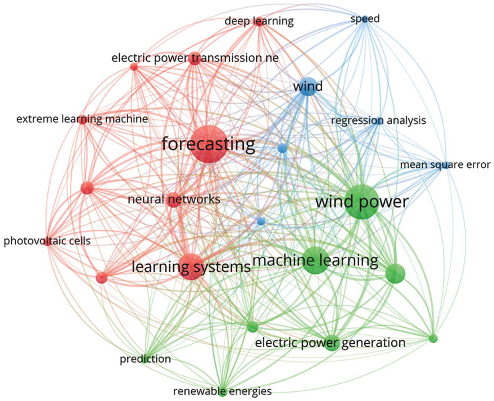
Figure 1: Bibliometric visualization of the keywords used in previous studies, created using VOSviewer
From all the above studies, it is clear that ML and DL algorithms are very useful in wind energy forecasting. However, it is still a very difficult thing to make an accurate prediction and a universal model is not possible. Therefore, every scenario requires a local dataset of wind speed, weather information, and location. Each model needs to be customized, built, and then trained. This accurate forecasting will help in the better management of demand and supply, smooth operation, flexibility and reliability and as well as economic implication.
In this research, a comparison has been made between different machine learning and DL forecasting algorithms for a day-ahead wind energy generation in Estonia. The historical data set on one-year Estonian wind energy generation was taken from the Estonian Transmission System operator (TSO) called ELERING [9]. This historical data contains all of the above-stated factors that affect wind energy generation. On the basis of this data, different forecasting algorithms are modeled, trained, and compared.
The key contributions of this paper are summarized as follows:
• To address the problem of wind energy forecasting in Estonia, state-of-the-art ML and DL algorithms are implemented and rigorously compared based on performance indices, such as root mean square error, computational complexity, and training time.
• A detailed exploratory data analysis is conducted for the selection of optimal models’ parameters, which proves to be an essential part of all implemented ML and DL algorithms.
• A total of six ML NAR and two DL algorithms are implemented, such as linear regression, tree regression, SVM, ARIMA, AR, NAR, ANFIS, and RNN-LSTM. All implemented algorithms are thoroughly compared with currently implemented TSO forecasted wind energy and our proposed RNN-LSTM forecasting algorithm proves to be a more accurate and effective solution based on performance indices.
The structure of the paper is shown in Fig. 2.
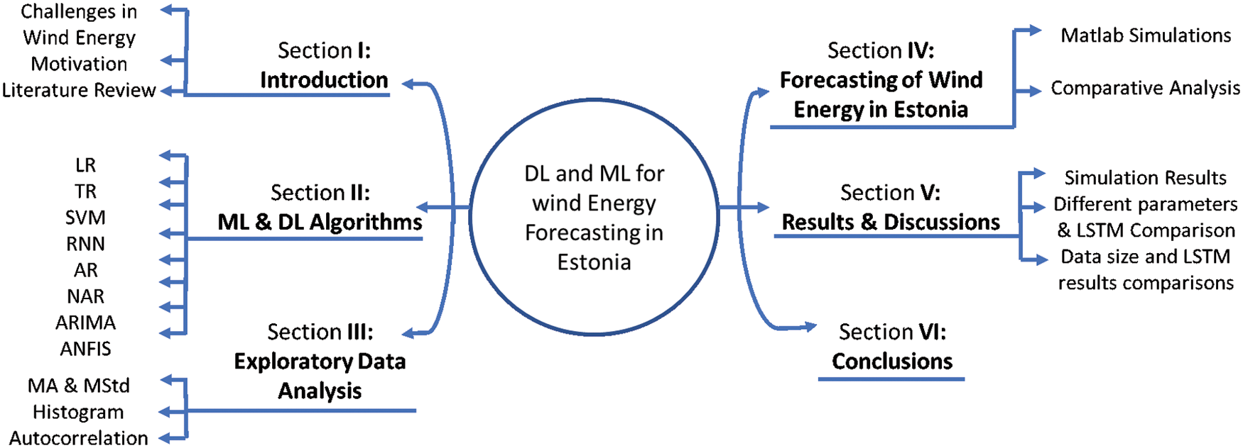
Figure 2: Paper outline
2 Machine Learning Algorithms for Forecasting
The most common ML tool for forecasting is regression-based algorithms [19]. Regression-based learning is categorized into supervised learning algorithms that use past data sets of the parameters in the training of the model and then predict the future values of the parameters based on the regressed time lag values of the parameters, where the number of lag selections is based on observation. Moreover, the most used DL algorithms in time series prediction are RNN and CNN. In CNN, the output only depends on the current input while in RNN, the output depends both on the current and previous values that provide an edge to RNN in time series prediction. In this section, machine learning and deep learning algorithms used in this study are elaborated.
This simplest and most commonly used algorithm computes a linear relationship between the output and input variables. The input variables can be more than one. The general equation for linear regression is along with its details can be found in [7].
This algorithm deploys a separate regression model for the different dependent variables, as these variables could belong to the same class. Then further trees are made at different time intervals for the independent variables. Finally, the sum of errors is compared and evaluated in each iteration, and this process continues until the lowest RMSE value is achieved. The general equation and the details of the algorithm are described in [7].
2.3 Support Vector Machine Regression (SVM)
SVM is another commonly used ML algorithm due to its accuracy. In SVM, an error margin called ‘epsilon’ is defined and the objective is to reduce epsilon in each iteration. An error tolerance threshold is used in each iteration as SVM is an approximate method. Moreover, in SVM, two sets of variables are defined along with their constraints by converting the primal objective function into a Lagrange function. Further details of this algorithm are given in [7,39,40]:
The RNN is usually categorized as a deep-learning algorithm. The RNN algorithm used in this paper is the Long Short-Term Memory (LSTM) [41]. In LSTM, the paths for long-distance gradient flow are built by the internal self-loops (recurrences). In this algorithm, to improve the abstract for long time series based different memory units are created. In conventional RNN, the gradient vanishing problem is a restriction on the RNN architecture to learn the dependencies of the current value on long-term data points. Therefore, in LSTM, the cell data are kept updated or deleted after every iteration to resolve the vanishing gradient issue. The LSTM network in this study consists of 200 hidden units that were selected based on the hit-and-trial method. After 200 hidden units, no improvement in the error is observed.
2.5 Autoregressive Neural Network (AR-NN)
This algorithm uses feedforward neural network architecture to forecast future values. This algorithm consists of three layers, and the forecasting is done iteratively. For a step ahead forecast, only the previous data is used. However, for the multistep ahead, previous data and forecasted results are also used, and this process is repeated until the forecast for the required prediction horizon is achieved. The mathematical relationship between input and output is as follows [42]:
where
2.6 Non-Linear Autoregressive Neural Network
The Nonlinear Autoregressive Neural Network (NAR-NN) predicts the future values of the time series by exploring the nonlinear regression between the given time series data. The predicted output values are the feedback/regressed back as an input for the prediction of new future values. The NA-NN network is designed and trained as an open-loop system. After training, it is converted into a closed-looped system to capture the nonlinear features of the generated output [43]. Network training is done by the backpropagation algorithm mainly by the step decent or Levenberg-Marquardt backpropagation procedure (LMBP) [44].
2.7 Autoregressive Integrated Moving Average (ARIMA)
This model is usually applied to such datasets that exhibit nonstationary patterns like wind energy datasets. There are mainly three parts of the ARIMA algorithm. The first part is AR where the output depends only on the input and its previous values. Eq. (3) defines an AR model for the p-order [45]:
where
The third part ‘I’ describes that the data have been updated by the amount of error calculated at each step to improve the efficiency of the algorithm. The final equation of ARIMA is as follows [45]:
2.8 Adaptive Neuro-Fuzzy Inference System (ANFIS)
This algorithm is a hybrid of ANN and Fuzzy logic. In the first step, Takagi and Sugeno Kang's fuzzy inference modeling method is used to develop the fuzzy system interference [46]. The overall model in this algorithm consists of three layers. The first and last layers are adaptable and can be modified accordingly to the design requirements while this middle layer is responsible for the ANN and its training. In the fuzzy logic interference system, the fuzzy logic structures and rules are defined. Moreover, it also includes fuzzification and defuzzification as well.
This algorithm works on Error Backpropagation (EPB) model. The model employs Least Square Estimator (LSE) in the last layer which optimizes the parameters of the fuzzy membership function. The EBP reduces the error in each iteration and then defines new ratios for the parameters to obtain optimized results. However, the learning algorithm is implemented in the first layer. The parameters defined in this method are usually linear [46,47].
Estonia is a Baltic country located in the northeastern part of Europe. Most of its energy is generated from fossil fuels, whereas the RESs are also contributing significantly. The distribution of RES and non-RES energy gen is shown in Fig. 1. The average share of fossil fuels is around 70% for the year 2019, while renewables are around 30% [9]. Although 30% is still higher as per the EU plan for renewable integration in the grid by 2020 [9]. As per the 35% share in RE, wind energy is the second most used resource in Estonia after biomass in 2019 [9], which makes it very important. The energy demand in Estonia is usually high in winter and the peak value is around 1500 MWh, while the average energy consumption is around 1000 MWh. Meanwhile, the average energy generation is around 600 MWh and the peak value is around 2000 MWh [9]. The demand and supply gap can vary between 200 to 600 MWh and is almost the same throughout the year. This gap is overcome by importing electricity from Finland, Latvia, and Russia if needed [9].
In Estonia, a total of 139 wind turbines are currently installed, mainly along the coast of the Baltic Sea [10]. Fig. 3 shows the geographical location of the installed sites. The installed capacity of these wind turbines is around 301 MW. In addition, there are 11 offshore and two offshore projects under the development phase. The plan is to have 1800 MW of wind power generation by the year 2030 [10]. The current share of wind energy is only around 10% of the total energy generated in Estonia. However, according to EU regulations, environmental factors, and self-dependency, this share will increase rapidly in the future. Therefore, due to the stochastic nature of wind speed, accurate prediction of wind power generation will be essential to manage demand and supply. A good and advanced prediction technique is required for an accurate wind power generation prediction in Estonia. This study provides a detailed and wide exploratory and comparative analysis for wind power generation forecasting by employing multiple linear and nonlinear ML and Deep Learning (DL) techniques.
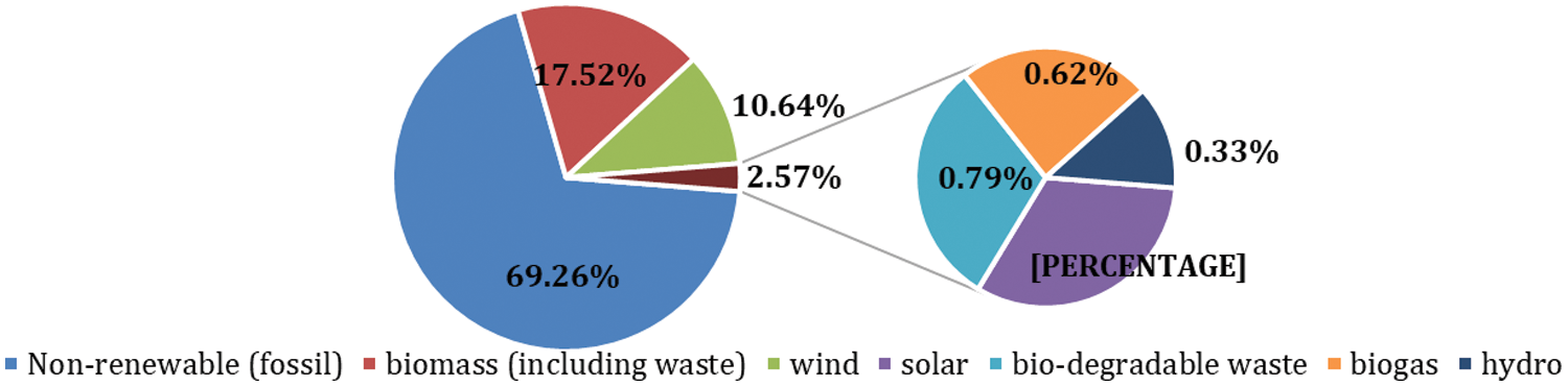
Figure 3: Share of renewable and non-renewable energy in Estonia
The data set used in this article is the Estonian general data on wind energy generation from 1 January 2011 to 31 May 2019. The frequency of the data set is one hour. This data set for wind energy generation is highly variable due to the weather conditions in Estonia. The maximum value of wind energy production in the aforementioned period is nearly 273 MWh, the mean value is 76.008 MWh, the median is 57.233 MWh, and the standard deviation is 61.861 MWh. To demonstrate the variable nature of the time series dataset for Estonian wind power generation, the moving average and the moving standard deviation are the best tools to elaborate on this dynamic nature of the dataset. Fig. 4 shows the wind energy production data along with the moving average and the moving standard deviation from Jan. 2018 to May 2019. It is clear from Fig. 4 that there are no clear peaks in wind energy or low seasonal values. Wind energy production is variable throughout the whole year. As indicated by the moving average, wind energy generation is high in winter (November to March), but even in that time, its value drops for a few weeks and then again increases.
The histogram and the probability density function (PDF) of the data are shown in Fig. 5a, which indicates that the wind energy production is below 50 MWh most of the time and its value rarely goes above 250 MWh. The histogram data is now normalized to compute the actual probability of different energy production values. The resultant probabilities are depicted in Fig. 5b. These probability values also indicate the same analogy. For example, the probability of getting 100 MWh energy is around 20% and 250 MWh is only around 3%. Therefore, the accuracy for the prediction of peak power generation or above-average power generation is a challenging task. Further analysis of this data set is performed using autocorrelation analysis. Fig. 5c shows the autocorrelation analysis of the data set.
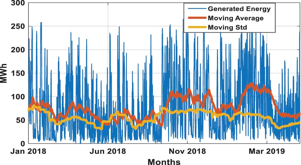
Figure 4: Energy production, moving average and moving std. deviation
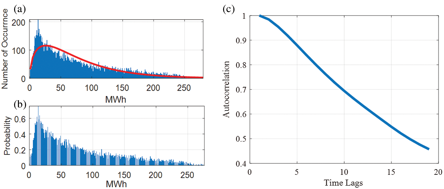
Figure 5: (a) Histogram (b) PDF of the data, (c) Autocorrelation analysis
In time-series analysis, the autocorrelation measure is a very useful tool to observe the regression nature of the time-series data and provides a birds-eye view for the election of the number of lags if any regression-based forecasting model is employed. It is the correlation of the signal with its delay version to check the dependency on the previous values. In this graph, the lag of 20 h is shown, in which the lags up to the previous 16 h have a regression value above 0.5 percent and after which it drops significantly below 0.5. The confidence interval is identified by the calculated 2 values. The correlation decreases slowly over time, which shows long-term dependency. The description of this observation is described in [48]. However, the autocorrelation of wind energy generation does not decrease rapidly with weather changes related to different seasons. This exploratory data analysis helps us to estimate design, and parameter selection for all ML and deep-learning algorithms defined earlier.
The Estonian wind energy dataset has been used in this research. The dataset is then divided into training, testing and validation and the divisions of data are 80%, 10% and 10%, respectively. All these simulations are carried out in Matlab2021a in a Windows 10 platform running on an Intel Core i7-9700 CPU with 64 GB RAM. Initially, the training data was converted into standard zero mean and unit variance form to avoid convergence in the data. The same procedure was carried out for the test data as well. The prediction features and response output parameter has also been defined for a multistep ahead furcating. The Estonian TSO is responsible for the forecasting of wind energy generation on an hourly basis. Their prediction algorithm forecasts wind energy generation 24 h in advance. It also generates the total energy production and the anticipated energy consumption. Fig. 6 shows the values of wind energy production and the values forecasted by the TSO algorithm for May 2019 [49].
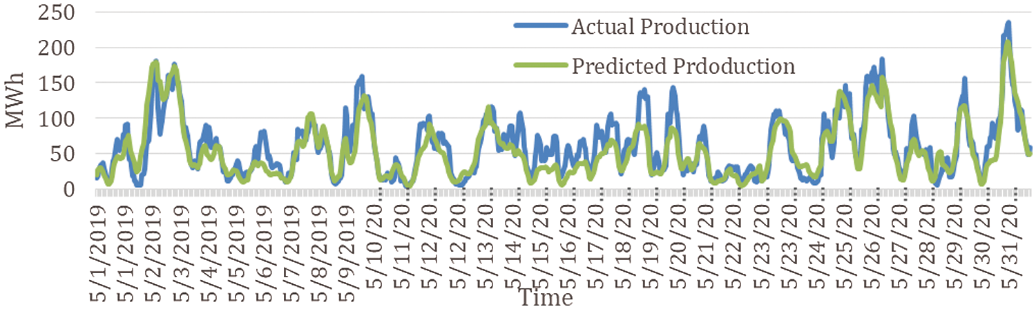
Figure 6: Actual and projected generation of wind energy in May 2019
Most of the time, the actual energy generation is much higher than the forecast values. The gap can go up to 70 MWh, which is too much. The forecasting algorithms need to be more accurate than that. This variation can falsely tell the energy supplier to use alternative energy sources rather than wind. This may be fossil fuel or any other resource, which will cost more to the supplier and eventually the customer. This low accuracy allowed us to study, develop, and propose a comparatively suitable forecasting algorithm for the prediction of wind power generation in Estonia.
In this study, the emphasis is on the accurate prediction of wind energy generation in Estonia. Eight different algorithms based on machine learning and DL are simulated and tested using the 1-year wind energy generation data set for a day-ahead prediction horizon. The results of all employed algorithms are compared based on RMSE values. Fig. 7 shows the comparison of actual wind energy generation and the forecast wind energy generation of TSO for 31 May 2019. It is clear from the figure that there is a substantial gap between the original and predicted values. The RMSE value for TSO forecasting is 20.432. The forecasting of all algorithms is tested on the same day as shown in Fig. 8.
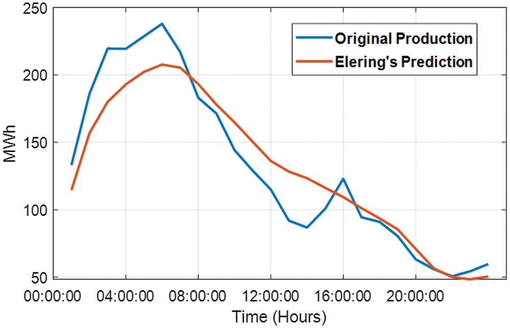
Figure 7: Wind energy actual vs. forecasted generation on May 31
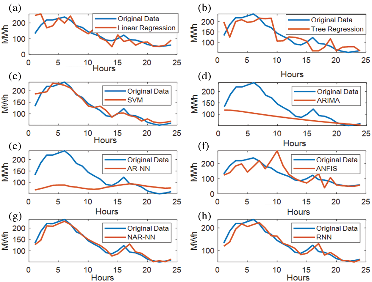
Figure 8: Forecasting of different algorithms: (a) Linear regression; (b) Tree Regression; (c) SVM; (d) ARIMA; (e) AR-NN; (f) ANFIS; (g) NAR-NN; (h) RNN-LSTM
The wind power generation data understudy has a highly nonlinear nature; therefore, a vast variety of linear and nonlinear forecasting algorithms need to be tested to find an appropriate option. A thorough comparative analysis is conducted to compare the accuracies of all forecasting algorithms employed in this paper. Machine learning algorithms, such as linear regression, AR, ARIMA, and tree-based regression, are not performed adequately, while SVM is given good forecast accuracy.
On the contrary, deep-learning algorithms, such as NAR and RNN, have a high degree of accuracy compared to all other algorithms employed as the architectures for both algorithms have the capability to capture nonlinear features of the data. However, the ANFIS also gives relatively low accuracy. The ML algorithms are not showing accuracy as the data is highly non-linear and therefore the ML algorithms do not perform better curve fitting and result in lower accuracy as compared to DL methods.
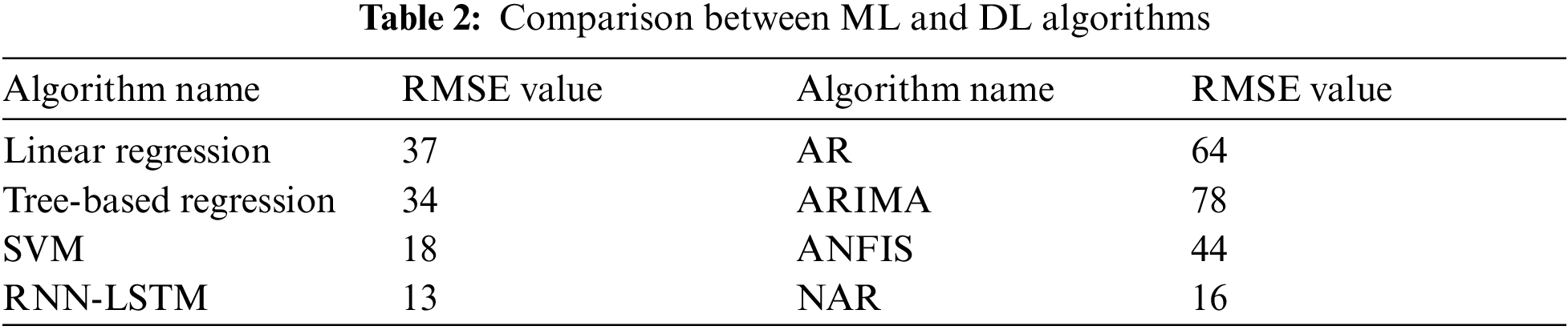
DL models, in contrast, due to the ANN fitted the curve better and therefore gave more accurate forecasting results. Thus, these results indicate that for this time series-based forecasting the efficiency of DL methods is higher as compared to ML methods. The comparative analysis of ML algorithms and DL algorithms based on the RMSE value is depicted in Tab. 2. In addition, to the best of the author's knowledge, this study is the first comprehensive comparative analysis between the know ML and DL algorithms for wind power generation data in Estonia.
Furthermore, it is pertinent to mention that this energy forecasting topic has been under investigation for decades. The main issue is still the accuracy of forecasting. The main focus is to forecast wind energy on the basis of past data and not wind speed. Some researchers have tried to develop some hybrid models as well. However, it is extremely difficult to compare the results of these studies with our study as there are many parameters involved like the size of the dataset, location, time span, and then the algorithm used.
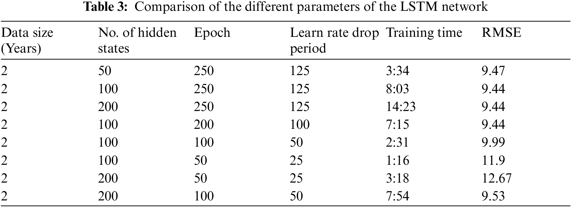
In this study, the best results are shown by the RNN-LSTM algorithm. The algorithm consists of 100 hidden units in the LSTM layer. This number of hidden units is obtained by the hit and trial method, the numbers are varied from 20 to 250. The models showed the best results for 100 units and after that, the results remained almost the same. It is using historical data only. Therefore, the number of features is one and the response is also one. The training of the algorithm is carried out by an ‘ADAM’ solver and the number of Epochs was also varied from 50–250 epochs. When the whole data set passes through the back or forward propagation through the neural network then it is called an Epoch. Learning rate is used to train the algorithm and when a certain number of Epochs are passed then it is dropped to a certain value. The initial learning rate was defined as 0.005. The gradient threshold is also one. The simulation parameters are described in Tab. 3.
In order to make multistep predictions, the prediction function makes a forecast of a single time step; and then updates the status of the network after each prediction. Now, the output of the first step will act as the input for the next step. The size of the data is also varied and tested between 1 month and 96 months to observe its impact on the forecasting algorithm. The simulation results show that after the data size is more than 24 months, the performance of this algorithm does not affect. Almost, the same RMSE value is obtained for 36, 60, and 96 months. The comparison is shown in Tab. 4. The RMSE values and the corresponding training time are also shown in Tab. 4.
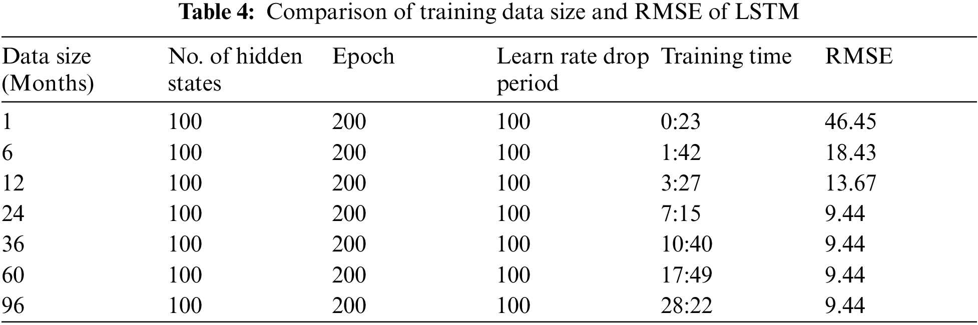
Fig. 9 shows the compression of actual wind energy production of TSO, the forecasted production and our algorithm for May 2019. It is clear from the graph that RNN-LSTM is providing better forecasts throughout the month. The RMSE value of the TSO furcating is 25.18 while the RNN forecasting is 15.20 for the whole month. Fig. 10a shows the error of both the TSO forecasting algorithm and the proposed RNN-LSTM algorithm. It is also clear from the graph that TSO's forecasting error is higher. The TSO's algorithm predicts a small variation in output energy well but fails when there are large fluctuations. On the other hand, RNN-LSTM is forecasting the large functional well but sometimes does not work that well with continuous low values of energy prediction. Therefore, a hybrid of both algorithms can be proposed here that will overcome both the low and high fluctuation. The results are shown in Fig. 10b. The error in forecasting is also depicted here. The error in forecasting is quite low now as is observed from the graph. The RMSE value for this hybrid forecasting is 8.69.
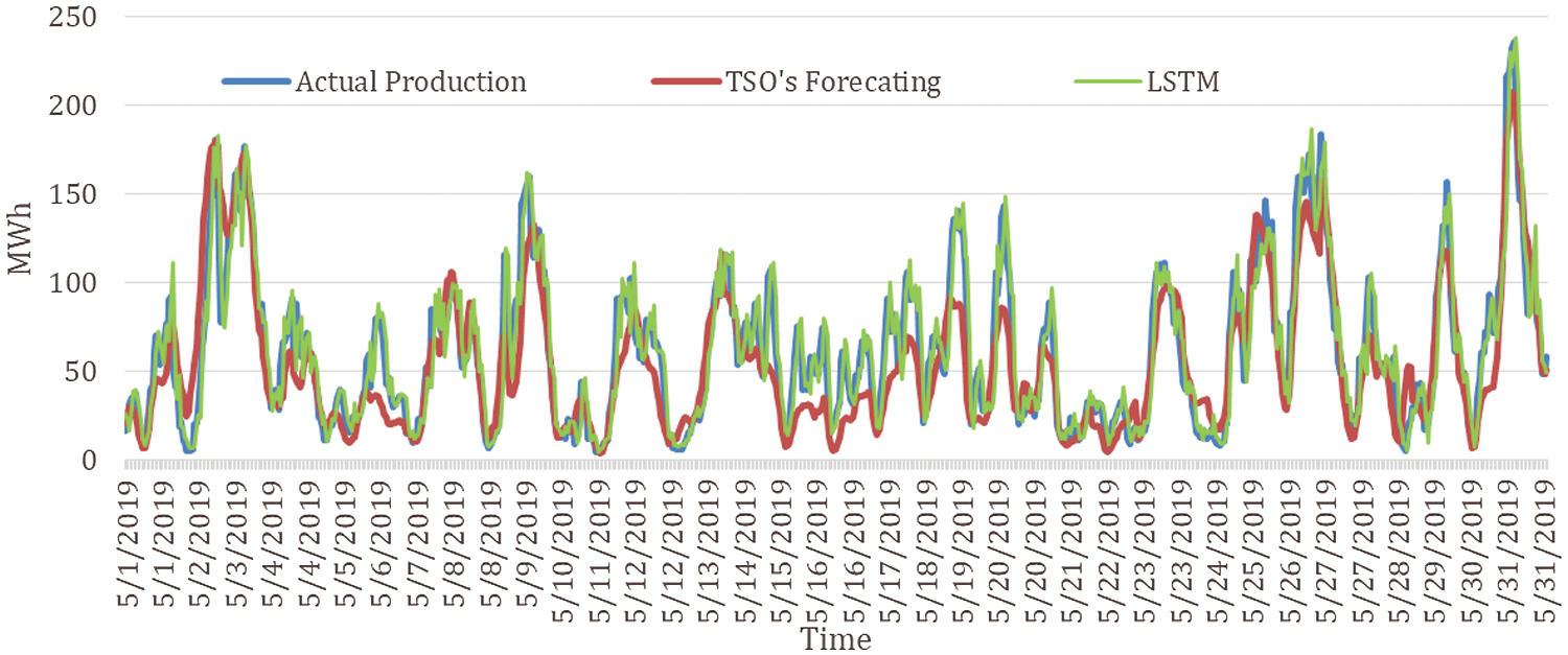
Figure 9: Comparison of wind energy actual generation, TSO's and RNN based forecast for May 2019
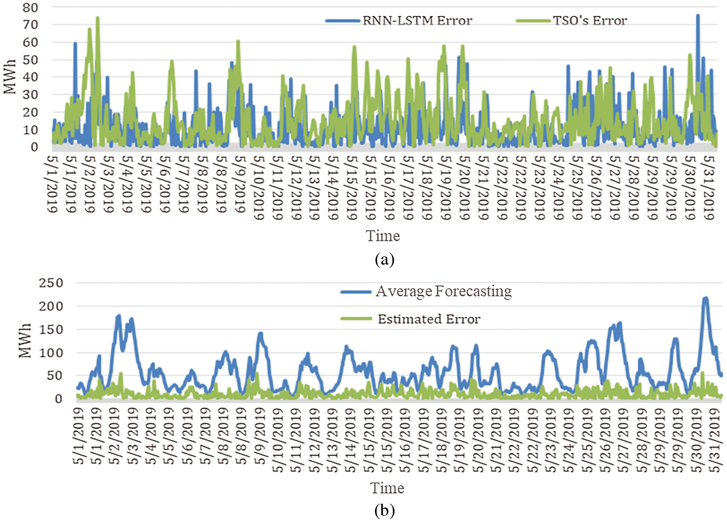
Figure 10: (a) Forecasting error of TSO's algorithm and LSTM forecasting; (b) Average value of both forecasting algorithms and error in average forecasting
In the past decade, ML and DL have become promising tools for forecasting problems. The highly nonlinear behavior of weather parameters especially wind speed makes it a valid challenging problem to use ML and DL algorithms for wind energy forecasting for smart grids. Moreover, an accurate time-series forecasting algorithm can help provide flexibility in modern grids and have economical and technical implications in terms of demand and supply management and for the study of power flow analysis in power transmission networks. In this paper, six ML and two DL forecasting algorithms are implemented and compared for Estonian wind energy generation data.
Wind energy accounts for approximately 35% of total renewable energy generation in Estonia. This is the first attempt to provide an effective forecasting solution for the Estonian energy sector to maintain power quality on the existing electricity grid. We target the day-ahead prediction horizon, which is the normal practice for the TSO forecasting wind energy model. Real-time year-long wind energy generation data are used for the comparative analysis of the ML and DL algorithms employed. Moreover, the results of all employed models are also compared with the forecasting results of TSO's algorithm. The comparison of all ML and DL algorithms is based on performance indices, such as RMSE, computational complexity, and training time. For example, the results for May 31, 2019, illustrated that TSO's forecasting algorithm has an RMSE value of 20.48. However, SVM, NAR, and RNN-LSTM have lower RMSE values. The results conclude that SVM, NAR, and RNN-LSTM are respectively 10%, 25%, and 32% more efficient compared to TSO's forecasting algorithm. Therefore, it is concluded that the RNN-LSTM based DL forecasting algorithm is the best-suited forecasting solution among all compared techniques for this case.
Acknowledgement: We acknowledge the support received from the Estonian Research Council Grants PSG142, PUT1680, Estonian Centre of Excellence in Zero Energy and Resource Efficient Smart Buildings and Districts ZEBE, Grant 2014-2020.4.01.15-0016 funded by European Regional Development Fund.
Funding Statement: This work was supported by the MSIT (Ministry of Science and ICT), Korea, under the ITRC (Information Technology Research Center) support program (IITP-2021-2016-0-00313) supervised by the IITP (Institute for Information & Communications Technology Planning & Evaluation).
Conflicts of Interest: The authors declare that they have no conflicts of interest to report regarding the present study.
1. X. Luo, J. Sun, L. Wang, W. Wang, W. Zhao et al., “Short-term wind speed forecasting via stacked extreme learning machine with generalized correntropy,” IEEE Transactions on Industrial Informatics, vol. 14, no. 11, pp. 4963–4971, 2018. [Google Scholar]
2. A. Hassan, A. U. Rehman, N. Shabbir, S. R. Hassan, M. T. Sadiq et al., “Impact of inertial response for the variable speed wind turbine,” in Proc. Int. Conf. on Engineering and Emerging Technologies, Lahore, Pakistan, pp. 1–6, 2019. [Google Scholar]
3. T. Mahmoud, Z. Y. Dong and J. Ma, “An advanced approach for optimal wind power generation prediction intervals by using self-adaptive evolutionary extreme learning machine,” Renewable Energy, vol. 126, pp. 254–269, 2018. [Google Scholar]
4. K. Mason, J. Duggan and E. Howley, “Forecasting energy demand, wind generation and carbon dioxide emissions in Ireland using evolutionary neural networks,” Energy, vol. 155, pp. 705–720, 2018. [Google Scholar]
5. A. M. Foley, P. G. Leahy, A. Marvuglia and E. J. McKeogh, “Current methods and advances in forecasting of wind power generation,” Renewable Energy, vol. 37, no. 1, pp. 1–8, 2012. [Google Scholar]
6. W. -Y. Chang, “A literature review of wind forecasting methods,” Journal of Power and Energy Engineering, vol. 2, no. 4, pp. 161–168, 2014. [Google Scholar]
7. N. Shabbir, R. Ahmadiahangar, L. Kütt and A. Rosin, “Comparison of machine learning based methods for residential load forecasting,” in Proc. Power Quality and Supply Reliability Conf. & Symp. on Electrical Engineering and Mechatronics, Kärdla, Estonia, pp. 1–4, 2019. [Google Scholar]
8. C. Wan, Z. Xu, P. Pinson, Z. Y. Dong and K. P. Wong, “Probabilistic forecasting of wind power generation using extreme learning machine,” IEEE Transactions on Power Systems, vol. 29, no. 3, pp. 1033–1044, 2014. [Google Scholar]
9. ELERING, Elering, 2019. [Online]. Available: https://elering.ee. [Google Scholar]
10. Estonian Wind Energy Association, Wind Energy in Estonia, 2019. [Online]. Available: http://www.tuuleenergia.ee/en/windpower-101/statistics-of-estonia/. [Google Scholar]
11. D. Mauree, R. Castello, G. Mancini, T. Nutta, T. Zhang et al., “Wind profile prediction in an urban canyon: A machine learning approach,” Journal of Physics: Conference Series, vol. 1343, no. 1, pp. 1–6, 2019. [Google Scholar]
12. H. Demolli, A. S. Dokuz, A. Ecemis and M. Gokcek, “Wind power forecasting based on daily wind speed data using machine learning algorithms,” Energy Conversion and Management, vol. 198, pp. 111823, 2019. [Google Scholar]
13. L. Zhang, K. Wang, W. Lin, T. Geng, Z. Lei et al.., “Wind power prediction based on improved genetic algorithm and support vector machine,” in Proc. IOP Conf. Series: Earth and Environmental Science, Bogor, Indonesia, pp. 32052, 2019. [Google Scholar]
14. T. Ahmad and H. Chen, “A review on machine learning forecasting growth trends and their real-time applications in different energy systems,” Sustainable Cities and Society, vol. 54, pp. 102010, 2020. [Google Scholar]
15. K. H. Tan, T. Logenthiran and W. L. Woo, “Forecasting of wind energy generation using self-organizing maps and extreme learning machines,” in Proc. IEEE TENCON, Penanag, Malaysia, pp. 451–454, 2017. [Google Scholar]
16. G. M. Khan, J. Ali and S. A. Mahmud, “Wind power forecasting an application of machine learning in renewable energy,” in Proc. Int. Joint Conf. on Neural Networks, Bejing, China, pp. 1130–1137, 2014. [Google Scholar]
17. H. Liu, X. Mi, Y. Li, Z. Duan and Y. Xu, “Smart wind speed deep learning based multi-step forecasting model using singular spectrum analysis, convolutional gated recurrent unit network and support vector regression,” Renewable Energy, vol. 143, pp. 842–854, 2019. [Google Scholar]
18. D. Zhang, X. Peng, K. Pan and Y. Liu, “A novel wind speed forecasting based on hybrid decomposition and online sequential outlier robust extreme learning machine,” Energy Conversion and Management, vol. 180, no. 2, pp. 338–357, 2019. [Google Scholar]
19. M. A. Khairalla, X. Ning, N. T. AL-Jallad and M. O. El-Faroug, “Short-term forecasting for energy consumption through stacking heterogeneous ensemble learning model,” Energies, vol. 11, no. 6, pp. 1–21, 2018. [Google Scholar]
20. G. Cocchi, L. Galli, G. Galvan, M. Sciandrone, M. Cantù et al., “Machine learning methods for short-term bid forecasting in the renewable energy market: A case study in Italy,” Wind Energy, vol. 21, no. 5, pp. 357–371, 2018. [Google Scholar]
21. A. Kumar and A. B. M. S. Ali, “Prospects of wind energy production in the western Fiji-An empirical study using machine learning forecasting algorithms,” in Proc. Australasian Universities Power Engineering Conf., Melbourne, Australia, pp. 1–5, 2018. [Google Scholar]
22. M. Ateeq, M. K. Afzal, M. Naeem, M. Shafiq and J. -G. Choi, “Deep learning-based multiparametric predictions for IoT,” Sustainability, vol. 12, no. 18, pp. 7752, 2020. [Google Scholar]
23. M. Sharifzadeh, A. Sikinioti-Lock and N. Shah, “Machine-learning methods for integrated renewable power generation: A comparative study of artificial neural networks, support vector regression, and Gaussian process regression,” Renewable & Sustainable Energy Reviews, vol. 108, pp. 513–538, 2019. [Google Scholar]
24. U. Cali and V. Sharma, “Short-term wind power forecasting using long-short term memory based recurrent neural network model and variable selection,” International Journal of Smart Grid and Clean Energy, vol. 8, no. 2, pp. 103–110, 2019. [Google Scholar]
25. G. L. T. Annael, J. Domingo, F. C. Garcia, M. L. Salvaña and N. J. C. Libatique, “Short term wind speed forecasting a machine learning based predictive analytics,” in Proc. Engineering Conf., Jeju Island, Korea, pp. 1948–1953, 2018. [Google Scholar]
26. M. Tahir, R. El-Shatshat and M. M. A. Salama, “Improved stacked ensemble based model for very short-term wind power forecasting,” in Proc. Int. Universities Power Engineering Conf., Glasgow, Scotland, pp. 1–6, 2018. [Google Scholar]
27. S. Balluff, J. Bendfeld and S. Krauter, “Short term wind and energy prediction for offshore wind farms using neural networks,” in Proc. Int. Conf. on Renewable Energy Research and Applications, vol. 5, Palermo, Italy, pp. 379–382, 2015. [Google Scholar]
28. D. Díaz–Vico, A. Torres–Barrán, A. Omari and J. R. Dorronsoro, “Deep neural networks for wind and solar energy prediction,” Neural Processing Letters, vol. 46, no. 3, pp. 829–844, 2017. [Google Scholar]
29. I. Okumus and A. Dinler, “Current status of wind energy forecasting and a hybrid method for hourly predictions,” Energy Conversion and Management, vol. 123, pp. 362–371, 2016. [Google Scholar]
30. A. Dupré, P. Drobinski, B. Alonzo, J. Badosa, C. Briard et al., “Sub-hourly forecasting of wind speed and wind energy,” Renewable Energy, vol. 145, pp. 2373–2379, 2020. [Google Scholar]
31. C. Chen and H. Liu, “Medium-term wind power forecasting based on multi-resolution multi-learner ensemble and adaptive model selection,” Energy Conversion and Management, vol. 206, pp. 112, 2020. [Google Scholar]
32. N. Shabbir, L. Kutt, M. Jawad, R. Amadiahanger, M. N. Iqbal et al.., “Wind energy forecasting using recurrent neural networks,” in Proc. IEEE Big Data, Knowledge & Control Systems Engineering, Sofia, Bulgaria, pp. 1–5, 2019. [Google Scholar]
33. M. A. Case, Y. Dong, L. Zhang, Z. Liu and J. Wang, “Integrated forecasting method for wind energy: A case study in China,” Processes, vol. 8, no. 35, pp. 1–26, 2020. [Google Scholar]
34. O. Abedinia, M. Bagheri, M. S. Naderi and N. Ghadimi, “A new combinatory approach for wind power forecasting,” IEEE Systems Journal, vol. 14, no. 3, pp. 4614–4625, 2020. [Google Scholar]
35. T. Esteoule, C. Bernon and M. Barthod, “Improving wind power forecasting through cooperation: A case-study on operating farms,” in Proc. Int. Conf. on Autonomous Agents and Multiagent Systems, Torronto, Canada, pp. 1940–1942, 2019. [Google Scholar]
36. D. Zafirakis, G. Tzanes and J. K. Kaldellis, “Forecasting of wind power generation with the use of artificial neural networks and support vector regression models,” Energy Procedia, vol. 159, pp. 509–514, 2019. [Google Scholar]
37. R. Yu, J. Cao, M. Yu, W. Lu, T. Xu et al., “LSTM-EFG for wind power forecasting based on sequential correlation features,” Future Generation Computer Systems, vol. 93, pp. 33–42, 2019. [Google Scholar]
38. S. Brusca, F. Famoso, R. Lanzafame, A. Galvagno, S. Mauro et al., “Wind farm power forecasting: New algorithms with simplified mathematical structure,” American Institute of Physics Conference Proceedings, vol. 21, no. 9, pp. 1–9, 2019. [Google Scholar]
39. MATLAB, Understanding Support Vector Machine Regression, 2020. [Online]. Available: https://se.mathworks.com/discovery/support-vector-machine.html. [Google Scholar]
40. N. Shabbir, R. Ahmadiahangar, L. Kutt, M. N. Iqbal and A. Rosin, “Forecasting short term wind energy generation using machine learning,” in Proc. Int. Scientific Conf. on Power and Electrical Engineering of Riga Technical University, Riga, Latvia, pp. 2019–2022, 2019. [Google Scholar]
41. N. Shabbir, M. Usman, M. Jawad, M. H. Zafar, M. N. Iqbal et al., “Economic analysis and impact on national grid by domestic photovoltaic system installations in Pakistan,” Renewable Energy, vol. 153, pp. 509–521, 2020. [Google Scholar]
42. T. D. Chaudhuri and I. Ghosh, “Artificial neural network and time series modeling based approach to forecasting the exchange rate in a multivariate framework,” Journal of Insurance and Financial management, vol. 1, no. 5, pp. 92–123, 2016. [Google Scholar]
43. MATLAB, Nonlinear autoregressive neural network, 2021. [Online]. Available: https://se.mathworks.com/help/deeplearning/ref/narnet.html. [Google Scholar]
44. MATLAB, NAR, 2021. [Online]. Available: https://se.mathworks.com/help/deeplearning/ref/narnet.html. [Google Scholar]
45. K. S. Sandhu and A. Ramachandran Nair, “A comparative study of arima and rnn for short term wind speed forecasting,” in Proc. Int. Conf. on Computing, Communication and Networking Technologies, Kanpur, India, pp. 8–14, 2019. [Google Scholar]
46. M. Jawad, A. Rafique, I. Khosa, I. Ghous, J. Akhtar et al., “Improving disturbance storm time index prediction using linear and nonlinear parametric models: A comprehensive analysis,” IEEE Transactions on Plasma Science, vol. 47, no. 2, pp. 1429–1444, 2019. [Google Scholar]
47. M. Jawad, S. M. Ali, B. Khan, U. faried, I. Sami et al., “Genetic algorithm-based non-linear auto-regressive with exogenous inputs neural network short-term and medium-term uncertainty modelling and prediction for electrical load and wind speed,” The Journal of Engineering, vol. 2018, no. 8, pp. 721–729, 2018. [Google Scholar]
48. T. Braun, M. Waechter, J. Peinke and T. Guhr, “Correlated power time series of individual wind turbines: A data driven model approach,” Journal of Renewable and Sustainable Energy, vol. 12, no. 2, pp. 1–13, 2020. [Google Scholar]
49. Elering, Wind Parks, 2021. [Online]. Available: https://dashboard.elering.ee/en/system/productionrenewable. [Google Scholar]
 | This work is licensed under a Creative Commons Attribution 4.0 International License, which permits unrestricted use, distribution, and reproduction in any medium, provided the original work is properly cited. |