DOI:10.32604/cmc.2022.024970
| Computers, Materials & Continua DOI:10.32604/cmc.2022.024970 | |
| Article |
Optimized Load Balancing Technique for Software Defined Network
1Department of Computer Science and Engineering, Chandigarh University, Mohali, Punjab, 140413, India
2School of Computational Sciences, CHRIST (Deemed to be University), Ghaziabad, 201003, India
3Department of Computer Science and Engineering, Sejong University, Seoul, 05006, Korea
4Department of Automotive ICT Convergence Engineering, Daegu Catholic University, Gyeongsan, 38430, Korea
*Corresponding Author: Woong Cho. Email: wcho@cu.ac.kr
Received: 06 November 2021; Accepted: 30 December 2021
Abstract: Software-defined networking is one of the progressive and prominent innovations in Information and Communications Technology. It mitigates the issues that our conventional network was experiencing. However, traffic data generated by various applications is increasing day by day. In addition, as an organization's digital transformation is accelerated, the amount of information to be processed inside the organization has increased explosively. It might be possible that a Software-Defined Network becomes a bottleneck and unavailable. Various models have been proposed in the literature to balance the load. However, most of the works consider only limited parameters and do not consider controller and transmission media loads. These loads also contribute to decreasing the performance of Software-Defined Networks. This work illustrates how a software-defined network can tackle the load at its software layer and give excellent results to distribute the load. We proposed a deep learning-dependent convolutional neural network-based load balancing technique to handle a software-defined network load. The simulation results show that the proposed model requires fewer resources as compared to existing machine learning-based load balancing techniques.
Keywords: SDN; software-defined networks; load balancing; performance enhancement
In today's era, traditional networks are unable to provide new services and fast innovation. Apart from this, the complexity of the network increases, which makes it harder to manage, and the data plane and control plane are coupled with each other as in router or switches. Software is deployed on dedicated hardware and, therefore, vendor-specific. Adding new Services requires costly new hardware. So, there is a need for a new approach to solving the issue discussed earlier. Therefore, a Software-defined Network (SDN) solves these problems, decoupling the control plane and information plane, making the network more agile, automated, open to all, and reducing business costs. However, today, the world is generating many data, it might be possible that the SDN network may get flooded with packets, and networks become congested and bottleneck. So, there is a need to balance the load in SDN [1]. Let us discuss the architecture of SDN. In SDN, a logically centralized controller controls several routing devices, as shown in Fig. 1 [1–3]. An important function of SDN architecture, given in Fig. 1, are as follows:
• Information Plane: Switching devices such as routers, switches, etc., are part of the information plane. It is responsible for processing and forwarding the packets as per the rules defined in the forwarding table.
• Controller plane: It is also known as “NETWORK BRAIN” and consists of controllers. It takes a decision where a packet is to be forwarded. The control plane's functions are system configuration, management, and routing table information exchange. It can be deployed in a different geographical area.
• Management plane: It is used for management and configure as per user's demand.
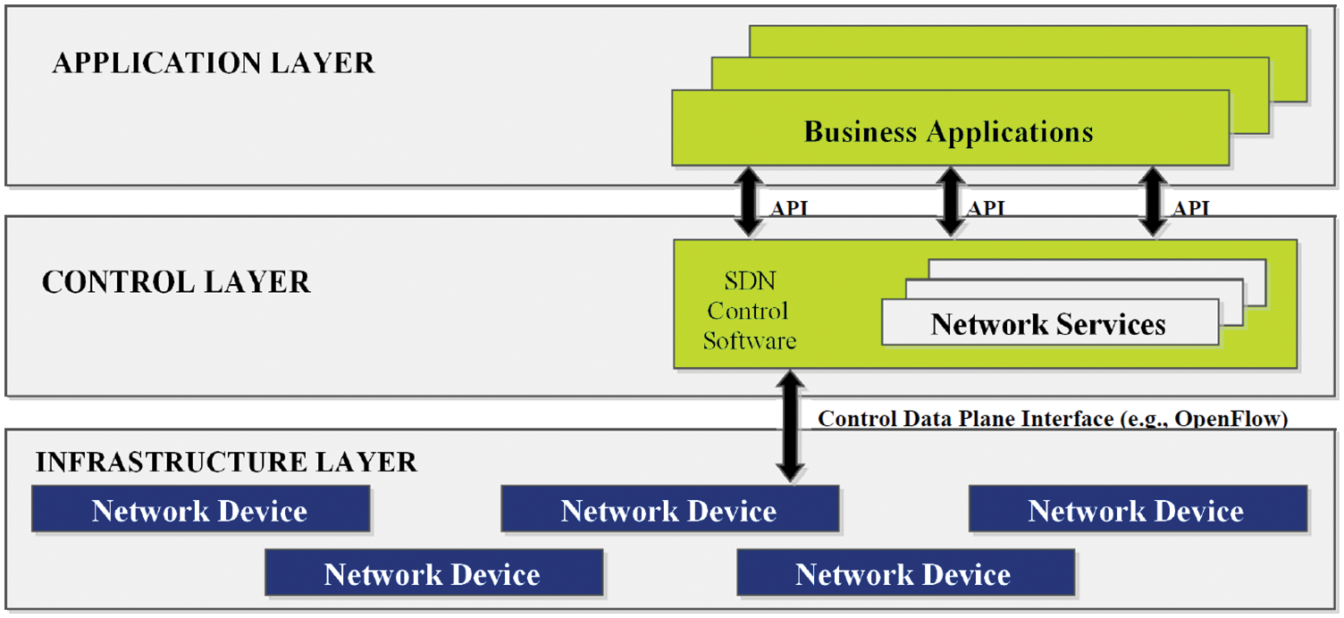
Figure 1: Software-defined architecture
Still, there was a problem with a standard protocol that helps communication between the information plane and controller plane. The OpenFlow protocol was created in 2008 to address the problem [4]. The Main Building blocks of Openflow are as follows:
• Flow table: It is the important component of OpenFlow switches/routers. When a packet arrives at a particular switch, the header field of the packet must match with flow table entries (shown in Fig. 2, which includes various phases, layers, and its header description [5].
• Port: Openflow characterized ports are capable of forwarding the packets to the controller, flooding, etc.
• Messages: The OpenFlow controller and switch represent messages that exchange between the OpenFlow controller and switches. Messages can be symmetric messages, asynchronous messages, or initiated by the controller. For example, PACKET IN, ECHO, PORT STATUS message.
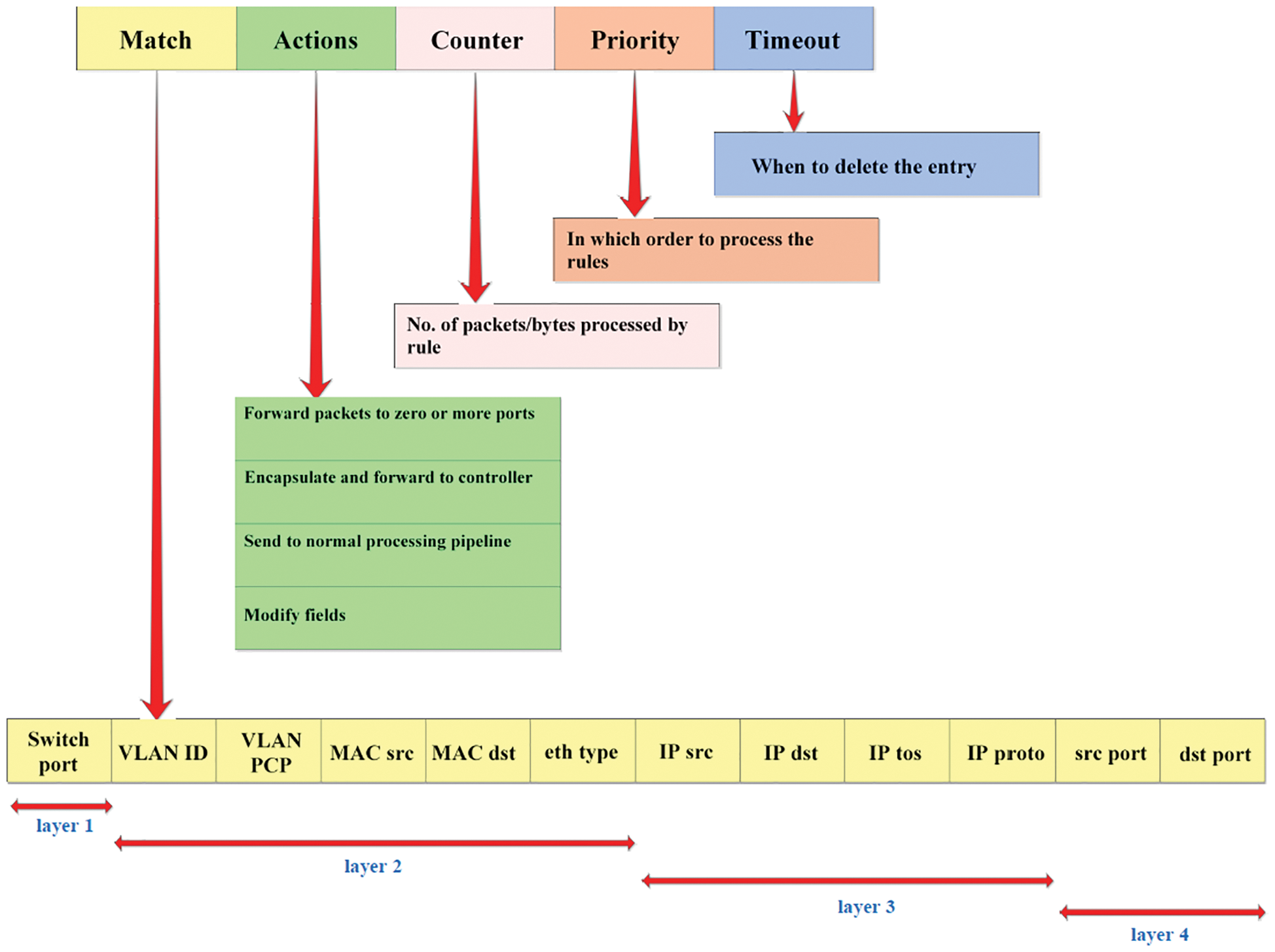
Figure 2: Structure of flow table
As illustrated in this manuscript, load-balancing is required through smart and intelligent algorithms that can tackle the load at its software layer and give excellent results to distribute the load. We propose a deep learning-dependent convolutional neural network (CNN)-based load balancing technique to handle the load in SDN. Further, we compare the test results with existing machine learning-based load balancing techniques.
An issue with SDN is that its controller can be overloaded by traffic. Therefore, we will discuss load balancing in the controller using a load balancer in SDN in a later section.
It is a procedure that is utilized to distribute the load among servers or any other computing device. Maximum throughput, minimum response time, maximum utilization of resources, avoiding overload, and avoiding crashing are the main objective of load balancing. Load balancing can be performed by hardware, software, or a combination of both. Dedicated software load balancers are manufacturer-specific and are costly. It can run on the hardware or virtual machine, as shown in Fig. 3. In our proposed methodology, we deal with the issue of load balancing.
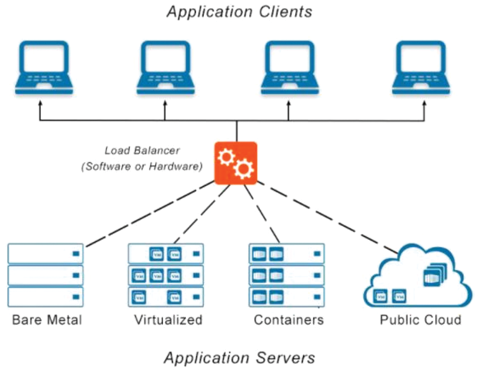
Figure 3: Load balancer
Intelligent Load balancing
In today's world, due to the huge increase in traffic, the demand of users, complexity of the application. Therefore, the business model needs to a robust, reliable, scalable, less complex, and adapt to new challenges with reduced cost. Hence there is a need for an intelligent load balancer. An intelligent load balancer distributes the packet or provides the optimized path considering various parameters. An intelligent load balancer can be achieved using Machine learning techniques. There are various machine learning techniques available, out of which we have taken a CNN to build our model.
This section looks at the research that has been published in the literature. It includes pros and cons, as well as the parameter they used for load balancing. Tab. 1 summarizes the algorithm used and the basis of the decision.
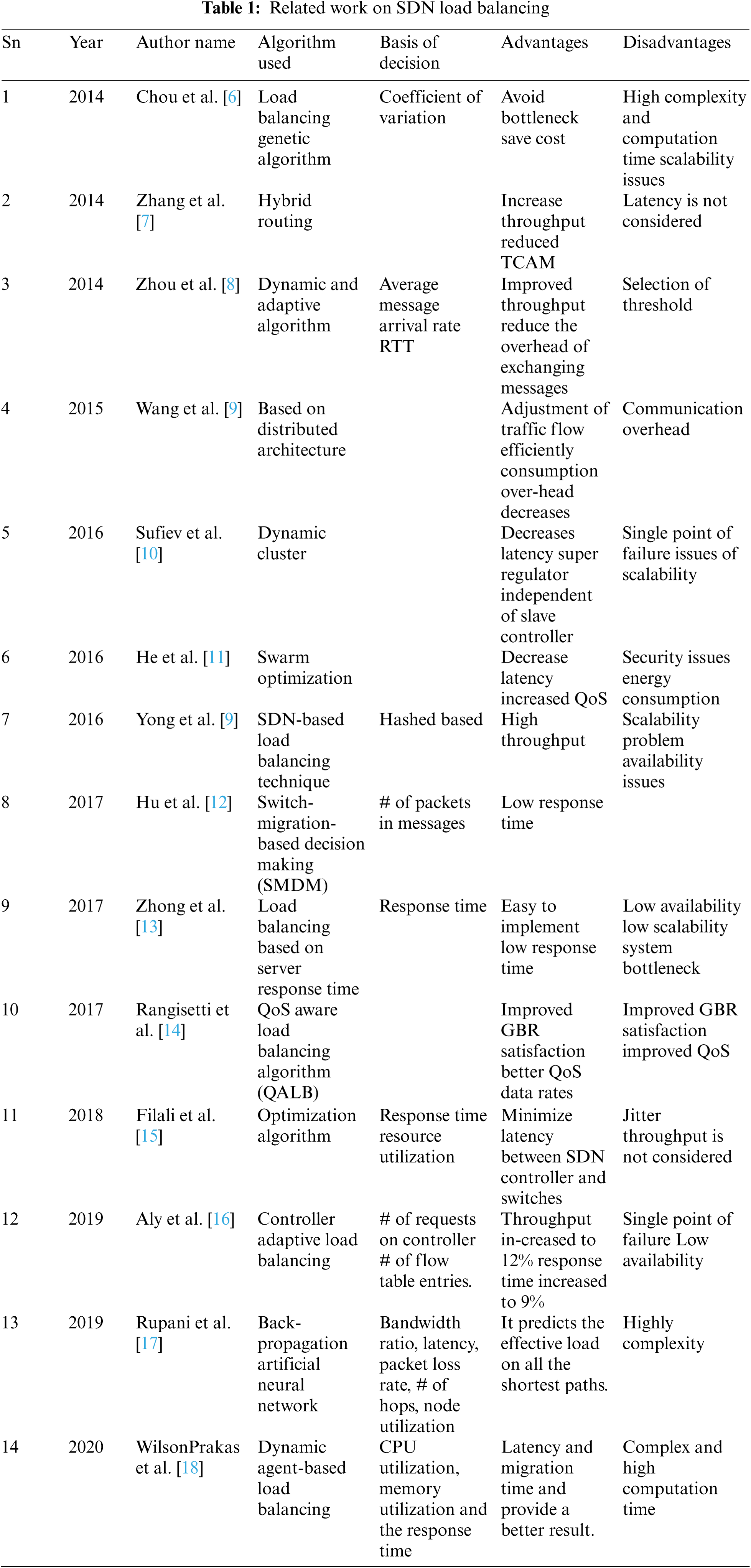
The details of Tab. 1 are described as follows: Li-Der Chou et al. presented an algorithm based on genetics, and a coefficient is utilized to assess the performance of the algorithm. They have selected the roulette-wheel selection, single-point cross-over, and single-point mutation and compared it with the round-robin algorithm [6].
Zhang et al. presented a strategy called Hybrid Routing. It uses both destination and explicit routing. In this methodology, the intricacy of the explicit routing diminishes, and the performance of the methodology is enhanced [7].
Zhou et al. proposed DALB (dynamic and adaptive algorithm) algorithm having distributed controller. This takes O(n) as overhead. It is tested on attributes such as throughput and average arrival time of the packet [8].
Wang et al. presented a load balancing methodology. The proposed model has three standard parts: a load collector, load balancer, and switch migrator. The load collector (Cbench) diverts the traffic to the controller. A controller has the threshold of the 70% of the controller information transmission [9]. At the point when the controller beats the threshold, the load balancer picks the controller (lightest weight).
Hadar Sufiev proposed a multi-regulator load adjusting model referred to as dynamic routing. Two sorts of controllers are the Super regulator and Regular regulator in the model. The load balancing occurs at two levels, one at the Super controller and the second at the Regular Controller. The super-controller continuously checks the gathering whether they have passed the threshold or not. On the off chance that when load passes the limit, at that point, the segment calculation runs [10].
He et al. combined fog computing with software-defined networks. Internet of Vehicles is integrated with Fog Computing-Software defined technology. The proposed methodology increases the QoS and reduces latency [11].
Hu et al. presented a load balancing technique called switch migration algorithm(SMDM). SMDM can be divided into three phases. At that point, it predicts migration costs and migration efficiency. It decides whether to carry out migration movement activities or not [12].
Zhong et al. introduced a methodology called Load Balancing Server Response Time (LBBSRT). It first gathers every server's reaction time at that point, picks the server, which has a steady reaction time. The proposed methodology is simple and efficiently balances the load among the controller and low response time [13].
Rangisetti et al. presented a combined version of Long-Term Evolution (LTE) Radio Access Network (RAN) and SDN and came up with a QALB algorithm. The algorithm calculates the neighboring cell's load, the user's QoS profile Equipment, and estimated throughput to balance the load. For more than 80 percent of the cell. The proposed algorithm provides a better QoS data rate [14].
Aly provided a load balancing methodology called controller adaptive load balancing (CALB). In this methodology, the super controller and slave controller are connected and, in turn, connected with n switches. It is used for both load balancing and fault tolerance [16].
Wilson Prakash et al. proposed an approach called Dynamic Agent-based load balancing (DALB), which is based on Backpropagation artificial neural network (BPANN) [15]. BPNN is integrated into the Controller agent. The BPNN takes the three inputs: CPU utilization, Memory utilization, and response time [18].
We propose an intelligent load balancing model (CNN 1D) for a software-defined network that takes 16 parameters, as discussed in the latter part of the section, including backward and forward parameters. We have used a convolution neural network that is less complex and takes less time than existing researcher models and machine learning models trained using KMeans. Let us discuss each element of the proposed model in detail.
Based on the previous work, we conclude that for load balancing, researchers take the load of the controller or take the load of transmission media. One thing common in both of them is that they have taken two or three-parameter for decision making. Nevertheless, not considered a load of transmission media and controllers load simultaneously. However, in our proposed methodology, we have considered both the loads and based on a CNN, we have used TensorFlow and Keras to implement the model. CNN is used because it is less complex and gives accurate results than other machine learning techniques.
Our main goal is to suggest a strategy for the Software-Defined System that considers all of the various parameters. The architecture of the suggested model is based on the dataset taken from the kaggle.com of Universidad Del Cauca Popayan, Colombia [19].
Clients send a request for a specific service to the server under our proposed method. It first passes the software load balancer, where the algorithm is implemented. Using CIC Flowmeter, the first algorithm will acquire flow statistics such as IP addresses, ports, inter-arrival periods, and so on. Based on these features, it determines the cluster value of the request and sends it to the relevant servers. In the following papes, we will go through each point in detail.
4.1 Process Flow of the Controller for SDN Traffic
In the proposed model, when a client sends a particular server service, it initially sends it to the controller. The load balancer checks the packet size of the packet and according to the flow statistics of both backward and forward direction of the flow captured using CIC Flowmeter. It will send to a router (server) based on the optimized results obtained through the CNN model and threshold of the router (server). Here, an important point to be considered is that the threshold of the router (server) is based on how many bytes per second it can process and the total number of the packet it can handle at any instance of time shown in Fig. 4. Let us examine the dataset used in the model in the following segment.
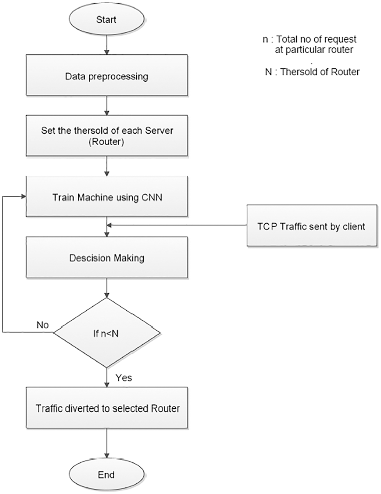
Figure 4: Proposed solution for software-defined network load balancing
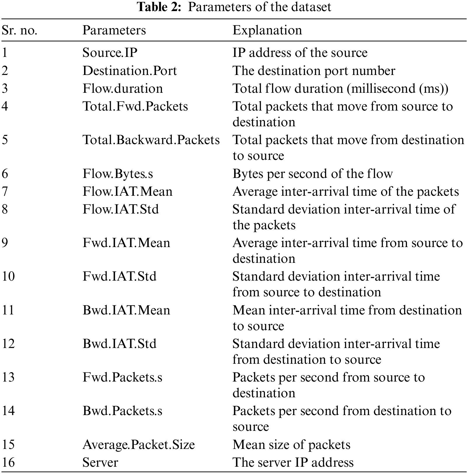
We used the dataset provided by Zhao et al. [19]. Fundamentally, it was caught from the Universidad Del Cauca, Popayan, Colombia United States of America. These data are from the TCP/UDP traffic caught at various hours on various days during the morning and evening of 2017. There is an aggregate of 3577296 packets. Out of these, 100000 packets are used to train our machine. This dataset has 87 features. We have taken 16 parameters to train and test the model, as shown in Tab. 2.
Visualization of the dataset is summarized in Fig. 5 [6]. Fig. 5 shows the correlation among the parameters and calculated using the Pearson correlation coefficient. In Fig. 6, all the parameters are taken on the x-axis and y-axis, generating correlations for exploratory analysis.
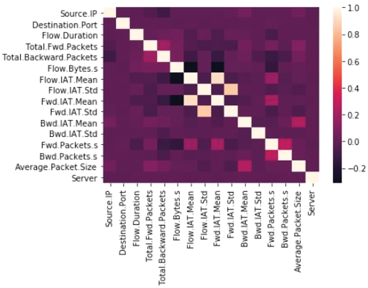
Figure 5: Correlation among the parameters in the dataset
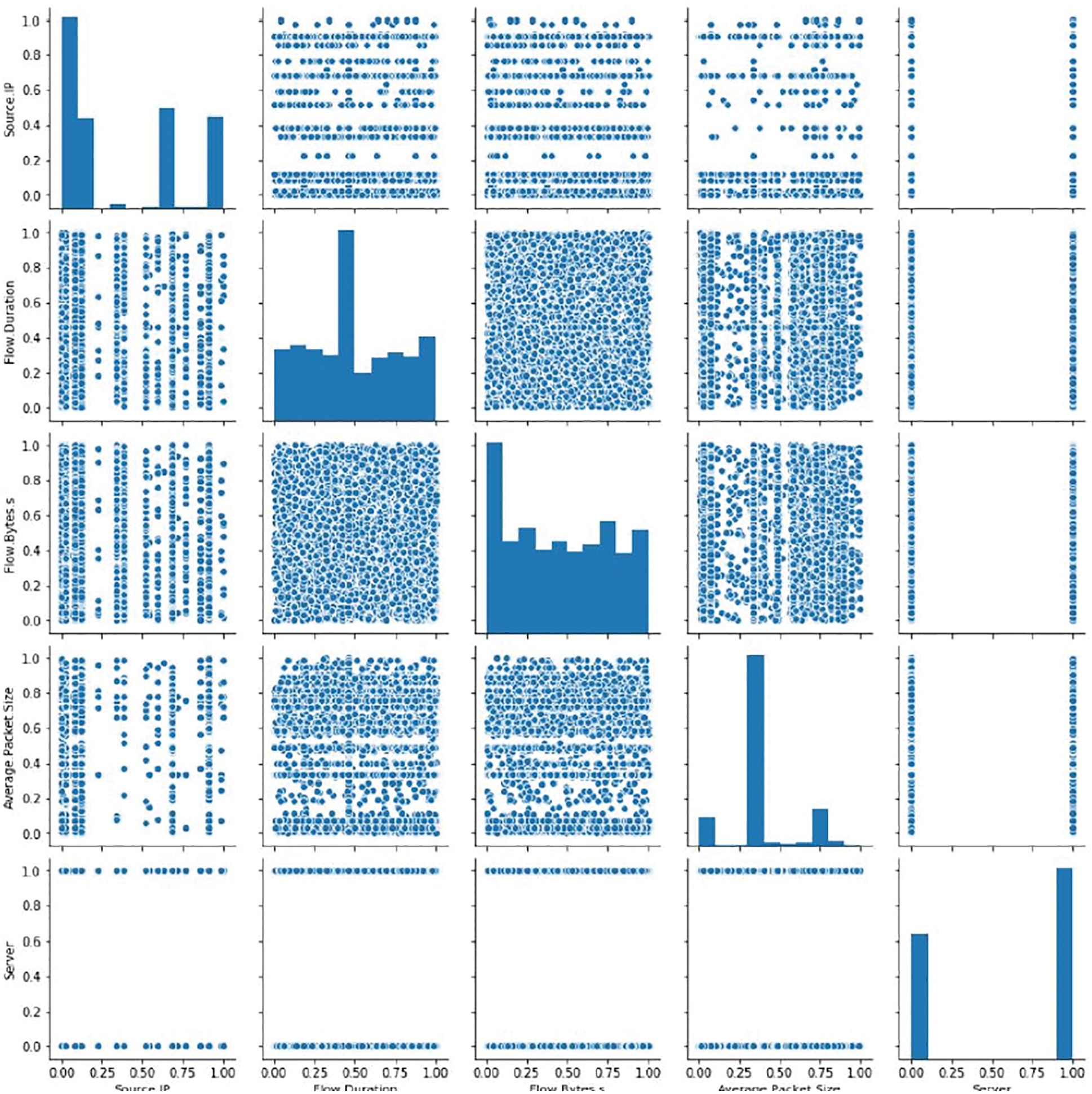
Figure 6: Dataset analysis
We took some parameters to visualize using the Seaborn module in Fig. 5. All the above statistics are helpful to perform Exploratory data analysis. In the following section, we will examine Data preprocessing.
Data preprocessing is the procedure to process the raw information with the goal that it tends to be utilized effectively with the three phases as Data Cleaning, Data Transformation, and Data Reduction
We first check the missing and boisterous information in our dataset, just as information sort of every parameter. These are accomplished by the panda's module, the Seaborn module of Python. Whatever we get the result, we performed hashing on this dataset. To standardize information, with the goal that it can lie somewhere in the range of 0 and 1. One of the famous and vital techniques to normalize the dataset is Min-Max scaling.
Min-max scalar formula is as follows:
where x is the ith value, max (x) and min (x) are maximum and minimum points in the particular column of a dataset, respectively, and z is the normalized value that lies between 0 to 1. This can be obtained by sklearn.preprocessing.MinMaxScaler class.
4.2 Convolutional Neural Network (CNN or ConvNets)
A CNN is a subset of deep learning which is inspired by biological processes where connectivity between neurons is similar to that of the animal cortex. Commonly used CNN is CNN 1D and CNN 2D.
COMMON LAYERS are: let us take an example of our model by running a CNN 1D on 16 features.
Input Layer: It contains input data of different dimensions and is based on CNN 1D, CNN 2D, etc.
Convolution Layer: The primary function detects the feature and yields the output by calculating the multiplication between filters and data size (in matrix form) as Fig. 6. Then slightly move the filter based on the stride size and perform the same operation. This process continues till we are at the end of the image. The output volume of the convolutional layer can be measured as:
where nl = Output dimension of lth layer, nl−1 = Output dimension of (l − 1)th layer, s[l] = Stride used in the layer, f[l] = Size of the filter, p[l−1] = Padding added of the l − 1 layer, As shown in Fig. 7 there is images of size nh × nw be 6 × 6 and the size of filter (f) = 3, stride (s) = 1 and padding (p) = 0.We overlap the filter to the information, perform component-wise multiplication, and add the outcome. Move the filter according to the stride and perform the same calculation until it reaches the end of the image.

Figure 7: Convolutional layer
Activation Function Layer: The activation function is applied to each element of the previous layer output. Examples are RELU. Sigmoid. Tanh, Leaky RELU, etc. The output remains unchanged. Here we have used RELU and Sigmoid function
Pooling Layer: The main objective is to diminish the size of the previous convolutional layer output, which makes the estimation fast, diminishes memory. There are two types of operation: max pooling and average pooling. It has three parameters, i.e., size, stride, and type of operations. An example of the Average pooling layer and Max pooling layer is shown in Fig. 8. Max pooling is a pooling activity that chooses the most significant component from the district of the element map secured by the filter. Average pooling registers the normal of the components present in the highlighted map area secured by the channel. Along these lines, while max-pooling gives the most conspicuous component in a specific fix of the element map, normal pooling gives the normal of highlights present in a fix.
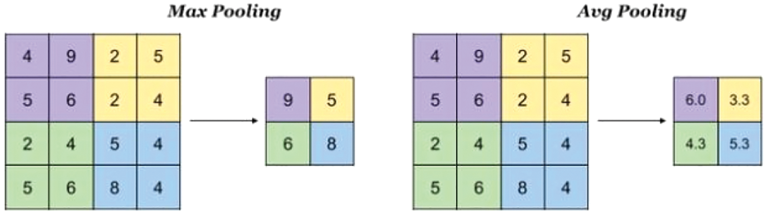
Figure 8: Pooling layer
Fully-Connected Layer: It is a deep neural system layer that takes contribution from the past layer and registers the class scores, and yields the 1-D cluster of size equal to the number of classes as shown in Fig. 9. All the layer that has been discussed with their output is shown in Fig. 10. In the proposed model, we have used two Convolution layers: conv1d 1 and conv1d 2. The output is obtained using Eq. (2). Here MAX POOLING is used(as depicted max pooling1d 1). Then we flatten the result obtained using MAX POOLING LAYER (shown as flatten) 1. We have used four dense layers (shown as dense 1, dense 2, dense 3, dense 4) and get the output in dense 4 layers (all the layers shown in Fig. 10.
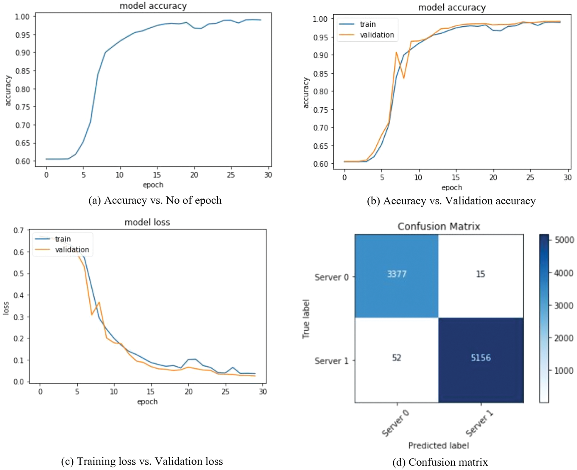
Figure 9: Performance of convolutional neural network model
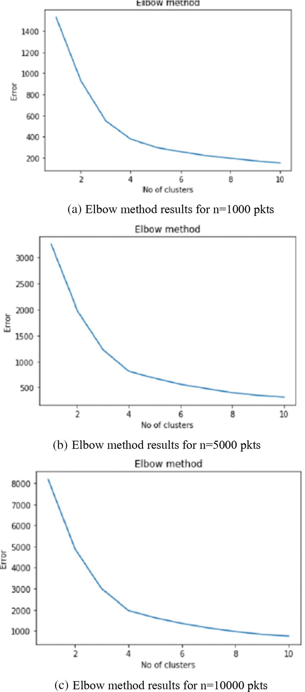
Figure 10: Elbow method in KMEANS
The Convolution neural network is trained on the training data for 30 epochs to get an accuracy of 98.94 percent, and testing is performed on 20 percent of the data. Here we have used the loss function as Binary cross entropy [20], while the Accuracy and Confusion matrix is used as a metric to test the model's accuracy. Now the forward and backward flow features (16 parameters) are used to obtain optimized results.
5.1 Training Results of CNN Model
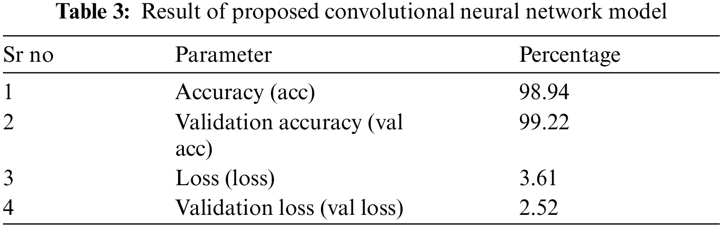
We tested the model on 43000 packets, out of which 20 percent are used for testing purposes, and the remaining 80 percent are used for training. The output has been shown in Figs. 10 and 11. In contrast, the performance has been illustrated in Fig. 10. A total of 9 layers are used to train the proposed model. We used 90, 60 filters in the convolution layer with a kernel size of 2, and in the pooling scenario, a pool size of two is used. The results are summarized in Tab. 3 and also shown in short form in Fig. 11.

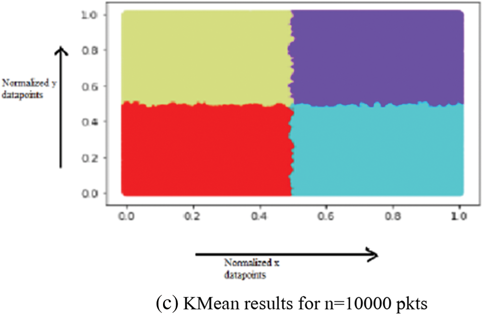
Figure 11: KMeans method in KMEANS (a) KMean results for n = 1000 pkts (b) KMean results for n = 5000 pkts (c) KMean results for n = 10000 pkts
We have our compared model with the Machine learning model trained using KMeans. It is tested on 5000, 10000, 20000, 50000 packets (shown in Figs. 10 and 11 First, in a machine learning model trained using KMeans, the elbow method is used to find an optimal number of servers (as shown in Fig. 10). The trained machine requires four servers to balance the load as concluded from the elbow method, and in Fig. 11, color legends show that numbers of servers and particular requests will go to the particular server.
The primary objective of any machine learning model is the efficiency parameters or performance parameters. The Tab. 3 illustrates the accuracy of the system is 98.94% while the validation accuracy for the system is more than 99%, i.e., 99.22%. It illustrates the correctness of the system. In terms of the loss percentage which is very important parameter specially for the loadbalancing techniques for software defined network. This loss parameter is 3.61% and therefore the final parameter is validation loss which is 2.52%. The clustering details are illustrated Figs. 10 and 11. The Fig. 10 is illustrating the elbow method to validate the number of clusters while the Fig. 11 is illustrating the clusters formed during the loadbalancing process. The system is tested for 1000, 5000 and 10000 packets respectively but the clutering is showing good in figure.
From this, we conclude that it requires four servers to balance the load obtained using KMeans, whereas our model can give optimized results on two servers only.
Load balancing is an essential and crucial mechanism for distributed computing-based technology in current network administration and application. A software-defined network is a technology to monitor and manage distributed computing requirements through various network management approaches, such as layered architecture, network virtualization, and orchestration. As the load is changed, the technique to handle this issue is also required to change. Therefore, we detailed the dynamic and intelligent method to handle load balancing for SDN in this work. The proposed techniques are based on deep learning, i.e., in particular, convolution neural networks. The proposed system is tested for an increasing load. The simulation results show that the proposed model performs better than the literature's existing static load balancing methods. We will plan to embed the code for the proposed technique through the SDN load balancer at the control plane.
Funding Statement: This work was supported by Ulsan Metropolitan City-ETRI joint cooperation Project [21AS1600], Development of intelligent technology for key industries and autonomous human-mobile-space autonomous collaboration intelligence technology].
Conflicts of Interest: The authors declare that they have no conflicts of interest to report regarding the present study.
1. D. Kreutz, F. M. Ramos and P. Verissimo, “Towards secure and dependable software-defined networks,” in Proc. of the Second ACM SIGCOMM Workshop on Hot Topics in Software-Defined Networking, Hong Kong, China, pp. 55–60, 2013. [Google Scholar]
2. B. Gardner, R. Sollmann, N. S. Kumar, D. Jathanna and K. U. Karanth, “State space and movement specification in open population spatial capture-recapture models,” Ecology and Evolution, vol. 8, pp. 10336–10344, 2018. [Google Scholar]
3. A. Kumar and D. Anand, “Load balancing for software defined network using machine learning,” Turkish Journal of Computer and Mathematics Education, vol. 12, no. 2, pp. 527–535, 2020. [Google Scholar]
4. N. McKeown, T. Anderson, H. Balakrishnan, G. Parulkar, L. Peterson et al., “OpenFlow: Enabling innovation in campus networks,” ACM SIGCOMM Computer Communication Review, vo, vol. 38, pp. 69–74, 2008. [Google Scholar]
5. M. Kuz’ niar, P. Perešíni and D. Kostic, “What you need to know about SDN flow tables,” in Int. Conf. on Passive and Active Network Measurement, New York, NY, USA, Springer, pp. 347–359, 2015. [Google Scholar]
6. L. D. Chou, Y. T. Yang, Y. M. Hong, J. K. Hu and B. A. Jean, “Genetic-based load balancing algorithm in OpenFlow network,” in Advanced Technologies, Embedded and Multimedia for Human-Centric Computing, Dordrecht, Netherlands: Springer, pp. 411–417, 2014. [Google Scholar]
7. J. Zhang, K. Xi, M. Luo and H. J. Chao, “Load balancing for multiple traffic matrices using SDN hybrid routing,” in Proc. IEEE 15th Int. Conf. on High-Performance Switching and Routing (HPSR), Paris, France, IEEE, pp. 44–49, 2014. [Google Scholar]
8. Y. Zhou, M. Zhu, L. Xiao, L. Ruan, W. Duan et al., “A load balancing strategy of SDN controller based on distributed decision,” in Proc. IEEE 13th Int. Conf. on Trust, Security and Privacy in Computing and Communications, Beijing, China, IEEE, pp. 851–856, 2014. [Google Scholar]
9. Y. Wang, X. Tao, Q. He and Y. Kuang, “A dynamic load balancing method of cloud-center based on SDN,” China Communications, vol. 13, pp. 130–137, 2016. [Google Scholar]
10. H. Sufiev and Y. Haddad, “A dynamic load balancing architecture for SDN,” in Proc. IEEE Int. Conf. on the Science of Electrical Engineering (ICSEE), Eilat, Israel, IEEE, pp. 1–3, 2016. [Google Scholar]
11. X. He, Z. Ren, C. Shi and J. Fang, “A novel load balancing strategy of software-defined cloud/fog networking in the internet of vehicles,” China Communications, vol. 13, pp. 140–149, 2016. [Google Scholar]
12. F. Hu, Q. Hao and K. Bao, “A survey on software-defined network and OpenFlow: From concept to implementation,” IEEE Communications Surveys & Tutorials, vol. 16, pp. 2181–2206, 2014. [Google Scholar]
13. H. Zhong, Y. Fang and J. Cui, “LBBSRT: An efficient SDN load balancing scheme based on server response time,” Future Generation Computer Systems, vol. 68, pp. 183–190, 2017. [Google Scholar]
14. A. K. Rangisetti and B. R. Tamma, “QoS aware load balance in software-defined LTE networks,” Computer Communications, vol. 97, pp. 52–71, 2017. [Google Scholar]
15. A. Filali, A. Kobbane, M. Elmachkour and S. Cherkaoui, “SDN controller assignment and load balancing with a minimum quota of processing capacity,” in Proc. IEEE Int. Conf. on Communications (ICC), Kansas City, MO, USA, IEEE, pp. 1–6, 2018. [Google Scholar]
16. W. H. F. Aly, “Controller adaptive load balancing for SDN networks,” in Proc. 11th Int. Conf. on Ubiquitous and Future Networks (ICUFN), Zagreb, Croatia, IEEE, pp. 514–519, 2019. [Google Scholar]
17. K. Rupani, N. Punjabi, M. Shamdasani and S. Chaudhari, “Dynamic load balancing in software-defined networks using machine learning,” in Proc. of Int. Conf. on Computational Science and Applications, Singapore, Springer, pp. 283–292, 2020. [Google Scholar]
18. S. WilsonPrakash and P. Deepalakshmi, “Artificial neural network based load balancing on software-defined networking”, in Proc. IEEE Int. Conf. on Intelligent Techniques in Control, Optimization and Signal Processing (INCOS), Tamilnadu, India, IEEE, pp. 1–4, 2019. [Google Scholar]
19. J. S. Rojas, “IP network traffic flows labeled with 75 apps,” Public Dataset. 2017. [Online]. Available: https://www.kaggle.com/jsrojas/ip-network-traffic-flows-labeled-with-87-apps. [Google Scholar]
20. J. Zhao, X. Mao and L. Chen, “Speech emotion recognition using deep 1D & 2D CNN LSTM networks,” Biomedical Signal Processing and Control, vol. 47, pp. 312–323, 2019. [Google Scholar]
 | This work is licensed under a Creative Commons Attribution 4.0 International License, which permits unrestricted use, distribution, and reproduction in any medium, provided the original work is properly cited. |