Computers, Materials & Continua DOI:10.32604/cmc.2022.025040
Article

Variational Bayesian Based IMM Robust GPS Navigation Filter

Dah-Jing Jwo1,* and Wei-Yeh Chang2

1Department of Communications, Navigation and Control Engineering, National Taiwan Ocean University Keelung, 202301, Taiwan
2TDK Taiwan Corp., Yangmei, Taoyuan, 326021, Taiwan
*Corresponding Author: Dah-Jing Jwo. Email: djjwo@mail.ntou.edu.tw
Received: 09 November 2021; Accepted: 27 December 2021

Abstract: This paper investigates the navigational performance of Global Positioning System (GPS) using the variational Bayesian (VB) based robust filter with interacting multiple model (IMM) adaptation as the navigation processor. The performance of the state estimation for GPS navigation processing using the family of Kalman filter (KF) may be degraded due to the fact that in practical situations the statistics of measurement noise might change. In the proposed algorithm, the adaptivity is achieved by estimating the time-varying noise covariance matrices based on VB learning using the probabilistic approach, where in each update step, both the system state and time-varying measurement noise were recognized as random variables to be estimated. The estimation is iterated recursively at each time to approximate the real joint posterior distribution of state using the VB learning. One of the two major classical adaptive Kalman filter (AKF) approaches that have been proposed for tuning the noise covariance matrices is the multiple model adaptive estimate (MMAE). The IMM algorithm uses two or more filters to process in parallel, where each filter corresponds to a different dynamic or measurement model. The robust Huber's M-estimation-based extended Kalman filter (HEKF) algorithm integrates both merits of the Huber M-estimation methodology and EKF. The robustness is enhanced by modifying the filter update based on Huber's M-estimation method in the filtering framework. The proposed algorithm, referred to as the interactive multi-model based variational Bayesian HEKF (IMM-VBHEKF), provides an effective way for effectively handling the errors with time-varying and outlying property of non-Gaussian interference errors, such as the multipath effect. Illustrative examples are given to demonstrate the navigation performance enhancement in terms of adaptivity and robustness at the expense of acceptable additional execution time.

Keywords: GPS; variational bayesian; Huber's M-estimation; interacting multiple model; adaptive; outlier; multipath

1  Introduction

Non-Gaussian noise is often encountered in many practical environments and the estimation performance deteriorates dramatically. Known to be one of the dominant error sources in high accuracy global navigation satellite systems (GNSS) [1] positioning systems, such as the Global Positioning System (GPS) [2,3], multipath effects [2,4] occur when GPS signals arrive at a receiver site via multiple paths due to reflections from nearby objects, such as the ground and water surfaces, buildings, vehicles, hills, trees, etc. Many estimation algorithms have been studied to eliminate the positioning error caused by multipath. Since multipath errors are among uncorrelated errors that are not cancelled out during observation differencing, the performance of high precision GPS receivers are mostly limited by the multipath induced errors. One of the most important issues in GPS system performance improvement is the interference suppression techniques.

The well-known Kalman filter (KF) [5] provides optimal estimate, namely minimum mean square error (MSE), of the system state vector and has been recognized as one of the most powerful state estimation techniques. As a recursive minimum norm estimation technique, the KF exhibits sensitivity to deviations from the assumed underlying probability distributions. Due to its simple structure, stable performance and low computational complexity, the conventional adaptive filtering algorithm where the least MSE is involved has been widely used in a variety of applications in the fields of adaptive signal processing and machine learning. However, the MSE criterion is limited to the assumption of linearity and Gaussianity while most of the noise in real word is non-Gaussian. The performance deteriorates significantly in the non-Gaussian noise environment. The traditional Kalman-type filter provides the best filter estimate when the noise is Gaussian, but most noise in real life is unknown, uncertain and non-Gaussian. The extended Kalman filter (EKF) is a nonlinear version of the KF and has been widely employed as the GPS navigation processor. The fact that EKF highly depends on a predefined dynamics model forms a major drawback. Furthermore, it is not optimal when the system is disturbed by heavy-tailed (or impulsive) non-Gaussian noises. To solve the performance degradation problem with non-Gaussian errors or heavy-tailed non-Gaussian noises, some robust Kalman filters have been developed by using non-minimum MSE criterion as the optimality criterion.

Essentially based on modification of the quadratic cost function in the filter framework, the Huber M-estimation methodology [6–9] provides between smooth norm properties for small residuals and robust norm properties for large residuals. The technique that relies on Huber's generalized maximum likelihood (ML) methodology exhibits robustness against deviations from the commonly assumed Gaussian probability density functions and can solve the non-Gaussian distribution problem efficiently and has been successfully employed for robust state estimation, inertial navigation system and visual tracking applications. The robust Huber's M-estimation-based EKF (HEKF) algorithm integrates both merits of the Huber M-estimation methodology and EKF. For the signals contaminated with non-Gaussian noises or outliers, a robust scheme combining the Huber M-estimation methodology and the EKF framework is beneficial where the Huber M-estimation methodology is used to reformulate the measurement information of the EKF to handle outliers and provide robustness against deviations from Gaussianity. The measurement update can be modified to enhance robustness using the Huber M-estimation methodology.

The variational Bayesian (VB) approach [10–15] is an inference method that utilizes a simple distribution to approximate the true posterior distribution of hidden variables, usually assuming that the hidden variables are independent of each other. The VB has been developed for a wide range of models to perform approximate posterior inference at low computational cost in comparison with the sampling methods. These methods assume a simpler, analytically tractable form for the posterior. The purpose of the variation is to find a variational distribution of the posterior probability density function (pdf) to minimize the Kullback-Leibler divergence (KLD) between the true posterior pdf. Two main approaches are either to derive a factored free form distribution or to assume a fixed form posterior distribution (e.g., a multivariate Gaussian, with possibly a suitable parametrization of the model).

The classical way of solving the problem of uncertain parameters is to use adaptive filters [16] where the model parameters or the noise statistics are estimated together with the dynamic states. The classical noise adaptive filtering approaches can be divided into Bayesian, maximum likelihood, correlation and covariance matching methods. The Bayesian approach is the most general of these and the other approaches can often be interpreted as approximations to the Bayesian approach. Examples of Bayesian approaches to noise adaptive filtering include state augmentation based methods, multiple model methods such as the interacting multiple model (IMM) algorithm [17–21]. The IMM algorithm has the configuration that runs in parallel several model-matched state estimation filters, which exchange information (namely interact) at each sampling time. The IMM algorithm has been originally applied to target tracking, and recently extended to navigation application. A model probability evaluator calculates the current probability of the vehicle being in each of the possible modes. A global estimate of the vehicle's state is computed using the latest mode probabilities. The algorithm carries out a soft-switching between the various modes by adjusting the probabilities of each mode, which are used as weightings in the combined global state estimate. The covariance matrix associated with this combined estimate takes into account the covariances of the mode-conditioned estimates as well as the differences between these estimates.

The algorithm proposed in this paper intends to provide an effective way for effectively handling the errors with time-varying and outlying property of non-Gaussian interference errors. The method utilizes the VB learning to approximate the noise strength for time-varying noise covariances, the Huber M-estimation methodology to enhance robustness especially for overcoming the problem of contamination distribution or outliers, and the IMM algorithm to furtherly tune the noise covariance matrices. The remaining of this paper is organized as follows. In Section 2, preliminary background on the Huber's M-estimation-based extended Kalman filter is reviewed. The variational Bayesian algorithm is discussed in Section 3. In Section 4, the interacting multiple model algorithm is presented. In Section 5, simulation experiments are carried out to evaluate the performance and effectiveness. Conclusions are given in Section 6.

2  Huber's M-Estimation-Based Extended Kalman Filter

For the nonlinear single model equations in discrete-time form, we have

xk=f(xk−1)+wk−1(1)

zk=h(xk)+vk(2)

where the state vector xk∈ℜn, process noise vector wk∈ℜm, measurement vector zk∈ℜm, measurement noise vector vk∈ℜm, Qk is the process noise covariance matrix and Rk is the measurement noise covariance matrix. The vectors wk and vk in Eqs. (1) and (2) are zero mean Gaussian white sequences has zero cross-correlation with each other:

E[wkwiT]=Qkδik;E[vkviT]=Rkδik;E[wkviT]=0 for all k and i(3)

where E[⋅] represents expectation, and superscript “ T” denotes matrix transpose. The symbol δik stands for the Dirac function:

δik={1,i=k0,i≠k

Based on robust strategy, the Huber M-estimation methodology possesses the ability to solve pollution distribution or outliers by improving filter update. The essence of Huber's robust estimation method is to solve the filter estimation value when the minimum cost function is obtained. For further applications, based on the generalized maximum likelihood estimation, a more general object function is given by Huber

J(x)=∑i=1mρ(υk,i)(4)

where ρ(⋅) is an appropriate positive symmetric function, υk,i is the residual. The cost function given by Huber is

ρ(υk,i)={12υk,i2|υk,i|<γγ|υk,i|−12γ2|υk,i|≥γ(5)

where γ is the default parameter. Amounts of experiences show that the performance is best when γ=1.345. For Huber's filtering robustness framework, reweighted average is used by

Ψk=diag[ψ(υk,i)],ψ(υk,i)=ϕ(υk,i)/υk,i(6)

where υk,i is the residual, ϕ(υk,i)=ρ′(υk,i) is the influence function.

The Huber M-estimation methodology makes use of the weighting matrix to recast the measurement information. The weighting matrix can be interpreted in terms of reweighting the residual error covariance and constructing the measurement process. The modified covariance has the form

R⌣k=RkT/2Ψk−1Rk1/2(7)

The HEKF algorithm is summarized as follow:

Stage 1: Prediction steps/time update equations

(1)   Predict the state vector

x^k|k−1=f(x^k−1)(8)

(2)   Predict the state error covariance matrix

Pk|k−1=ΦkPk−1ΦkT+Qk(9)

Stage 2: Correction steps/measurement update equations

(3)   Compute the residual

υk=(Rk)−1/2(zk−h(x^k|k−1))(10)

(4)   Compute the reweighting covariance matrix for measurement noise

R⌣k=RkT/2Ψk−1Rk1/2(11)

(5)   Compute Kalman gain matrix

Kk=Pk|k−1HkT(HkPk|k−1HkT+R⌣k)−1(12)

(6)   Update state vector

x^k=x^k|k−1+Kk(zk−h(x^k|k−1))(13)

(7)   Update state error covariance matrix

Pk=(I−KkHk)Pk|k−1(14)

3  The Variational Bayesian Approach

The variational Bayesian approach is an inference method that utilizes a simple distribution to approximate the true posterior distribution of hidden variables to find a variational distribution of the posterior probability density function (pdf) to minimize the KLD between the true posterior pdf. The variable decibel parameter is estimated by iterative calculations in which the gradient descent algorithm is involved. The difference between the lower bounds of two adjacent repeated calculations is used as the basis for judging convergence.

3.1 Variational Bayesian Extended Kalman Filter

Based on the Bayesian rule, the posterior distribution of the system state and the measurement noise covariance can be represented as

p(xk,Rk|z1:k)=p(xk,Rk,z1:k)p(z1:k)=p(zk,z1:k−1|xk,Rk)p(xk,Rk)p(zk,z1:k−1)=p(zk|z1:k−1,xk,Rk)p(z1:k−1|xk,Rk)p(xk,Rk)p(zk|z1:k−1)p(z1:k−1)=p(zk|z1:k−1,xk,Rk)p(xk,Rk|z1:k−1)p(zk|z1:k−1)=p(zk|xk,Rk)p(xk,Rk|z1:k−1)p(zk|z1:k−1)(15)

which can be simplified to p(zk|xk,Rk). For the first-order Markov process

p(xk,xk−1,Rk,Rk−1|z1:k−1)=p(xk|xk−1)⋅p(Rk|Rk−1)p(xk−1,Rk−1|z1:k−1)(16)

the Chapman-Kolmogorov equation can be obtained through the integration.

p(xk,Rk|z1:k−1)=∬p(xk|xk−1)⋅p(Rk|Rk−1)p(xk−1,Rk−1|z1:k−1)dxk−1dRk−1(17)

Given the next measurement zk, the predictive distribution is updated to a posterior distribution using the Bayes rule

p(xk,Rk|z1:k)∝p(zk|xk,Rk)p(xk,Rk|z1:k−1)(18)

The conditional probability distribution can be approximated as a product of Gaussian and Inverse-Gamma distributions

p(xk,Rk|z1:k−1)≈N(x^k|k−1,Pk|k−1)⋅∏i=1dIG(σk,i2;αk|k−1,i,βk|k−1,i)(19)

where N(x^k|k−1,Pk|k−1) is the Gaussian distribution for prediction xk with parameters x^k|k−1 and Pk|k−1. αk|k−1,i, βk|k−1,i are two parameters of the Inverse-Gamma distribution for σk,i2, the i-th diagonal element of Rk.

The variational Bayesian extended Kalman filter (VBEKF) employes a heuristic approach in the calculation process and predicts the distribution parameter by the first-order approximation

αk|k−1,i=ρiαk−1,i,βk|k−1,i=ρiβk−1,i,i=1,…,d(20)

The parameters of the new distribution is updated through

αk,i=12+αk|k−1,i,i=1,…,d(21)

βk,i=βk|k−1,i+12{Exk[(zk−h(x^k))(zk−h(x^k))T]}ii,i=1,…,d(22)

and the measurement noise variance can be estimated

R^k=E[Rk]=diag{E[σk,12],E[σk,22],⋯,E[σk,d2]}=diag[βk,1/αk,1,βk,2/αk,2,⋯,βk,d/αk,d],i=1,…,d=diag[βk,i/αk,i](23)

The VBEKF algorithm is summarized as follows:

Stage 1: Prediction steps/time update equations

(1)   Predict the state vector:

        x^k|k−1=f(x^k−1)

(2)   Predict the state error covariance matrix

        Pk|k−1=ΦkPk−1ΦkT+Qk

(3)   Predict the distribution parameter

        αk|k−1,i=ρiαk−1,i,βk|k−1,i=ρiβk−1,i,i=1,…,d(24)

Stage 2: Correction steps/measurement update equations

Set xk(0)=x^k|k−1,Pk(0)=Pk|k−1,αk,i=1/2+αk|k−1,i,βk,i(0)=βk|k−1,i, and start iteration loop:

(4)   Compute measurement noise variance

        R^kN=diag(βk,iN/αk,i)(25)

(5)   Compute Kalman gain matrix

        KkN=Pk|k−1HkT(HkPk|k−1HkT+R^kN)−1

(6)   Update state vector

        x^kN=x^k|k−1+KkN(zk−h(x^k|k−1))

(7)   Update state error covariance matrix

        PkN=(I−KkNHk)Pk|k−1

(8)   Update the measurement distribution parameter

        βk,iN=βk|k−1,i+12[(zk−h(x^kN))i2+(HkPkNHkT)ii](26)

Set x^k=x^kN,Pk=PkN,βk,i=βk,iN, go back to Step (4) until convergence.

3.2 Variational Bayesian Huber's M-Estimation Based Extended Kalman Filter

The positioning accuracy is degraded due to the presence of outliers and time-varying noise strength. Incorporation of the VB and Huber M-estimation methodologies into the EKF yielding the variational Bayesian Huber's M-estimation based extended Kalman filter (VBHEKF) algorithm can effectively overcome the outliers and time-varying variance in the measurement noise and improve the positioning accuracy. The VBHEKF algorithm is summarized as follows:

Stage 1: Prediction steps/time update equations

(1)   Predict the state vector

        x^k|k−1=f(x^k−1)

(2)   Predict the state error covariance matrix

        Pk|k−1=ΦkPk−1ΦkT+Qk

(3)   Predict the distribution parameters

        αk|k−1,i=ρiαk−1,i,βk|k−1,i=ρiβk−1,i,i=1,…,d(27)

Stage 2: Correction steps/measurement update equations

Set xk(0)=x^k|k−1,Pk(0)=Pk|k−1,αk,i=1/2+αk|k−1,i,βk,i(0)=βk|k−1,i, and start iteration loop:

(4)   Compute measurement noise variance:

        R^kN=diag(βk,iN/αk,i)(28)

(5)   Compute the residual

        υk=(R^kN)−1/2(zk−h(x^k|k−1))(29)

(6)   Compute the reweighting covariance matrix for measurement noise

        R⌣k=RkT/2Ψk−1Rk1/2(30)

(7)   Compute Kalman gain matrix

        KkN=Pk|k−1HkT(HkPk|k−1HkT+R⌣k)−1(31)

(8)   Update state vector

        x^kN=x^k|k−1+KkN(zk−h(x^k|k−1))(32)

(9)   Update state error covariance matrix

        PkN=(I−KkNHk)Pk|k−1(33)

(10)   Update the measurement distribution parameter

        βk,iN=βk|k−1,i+12[(zk−h(x^kN))i2+(HkPkNHkT)ii](34)

Set x^k=x^kN,Pk=PkN,βk,i=βk,iN, go back to Step (4) until convergence.

4  Interacting Multiple Model Extended Kalman Filter

Based on pseudo-Bayesian theory, the IMM algorithm employs two or more filters to process in parallel where each filter corresponds to a different state space or measurement model. It is an adaptive mechanism which dynamically identifies uncertainties or modeling errors can be adopted and is mainly an algorithm involving Markov chain switching coefficients between different models. In each model an EKF is running, and the IMM algorithm makes uses of model probabilities to weight the inputs and output of a bank of parallel filters at each time instant.

Assuming that a target with r states, corresponding to r models, set the system state equation and system observation equation represented by the j-th model are as follows:

xkj=f(xkj)+wk−1j(35)

zk=h(xk)+vk(36)

where the state vector xk∈ℜn, process noise vector wk∈ℜm, measurement vector zk∈ℜm, measurement noise vector vk∈ℜm, Qk is the process noise covariance matrix and Rk is the measurement noise covariance matrix. The vectors wk and vk in Eqs. (35) and (36) are zero mean Gaussian white sequences has zero cross-correlation with each other:

E[wkwiT]=Qkδik;E[vkviT]=Rkδik;E[wkviT]=0for all k and i

where E[⋅] represents expectation, and superscript “ T” denotes matrix transpose. The symbol δik stands for the Dirac function:

δik={1,i=k0,i≠k

The IMM-EKF algorithm is summarized as follows:

        Stage 1: Model interaction/mixing

Compute mixed state and corresponding covariances of model j

x^k−10j=∑i=1rx^k−1|k−1iμk−1ij(37)

Pk−10j=∑i=1rμk−1ij{Pk−1|k−1i+[x^k−1|k−1i−x^k−10j][x^k−1|k−1i−x^k−10j]T}(38)

where μk−1ij=∑i=1r1c¯jpijμk−1i and c¯j=∑i=1rpijμk−1i.

        Stage 2: Model filtering

x^k|k−1j=f(x^k−1ij)(39)

Pk|k−1j=ΦkjPk−10jΦkjT+Qkj(40)

Kkj=Pk|k−1jHkT(HkPk|k−1jHkT+Rk)−1(41)

x^kj=x^k|k−1j+Kkj(zk−h(x^k|k−1j))(42)

Pkj=(I−KkjHk)Pk|k−1j(43)

        Stage 3: Model probabilities update

Compute the likelihood function

Λkj=1(2π)n2|Skj|12exp⁡{−12vjT(Skj)−1vj}(44)

where vj=zk−h(x^k|k−1j) and Skj=HkPk|k−1jHkT+Rk. The model probability is updated according to the model likelihood and model transition probability

μkj=Λkjc¯jc(45)

c=∑j=1rΛkjc¯(46)

        Stage 4: Combination of model estimates and covariances

x^k=∑j=1rx^kjμkj(47)

Pk=∑j = 1rμkj{Pkj+[x^kj−x^k]⋅[x^kj−x^k]T}(48)

The algorithm performs real-time detection by setting model filters corresponding to the number of possible models, setting weight coefficients and model update probabilities for each filter, and finally performing weighted fusion to calculate the current optimal system state estimation to achieve the purpose of model adaptation.

5  Illustrative Examples

To validate the effectiveness of the proposed approaches, simulation experiments have been carried out to evaluate the performance of the proposed approach in comparison with the other conventional methods for GPS navigation processing. The computer codes were developed by the authors using the Matlab® software. The commercial software Satellite Navigation (SatNav) Toolbox by GPSoft LLC [22] was employed for generation of the GPS satellite orbits/positions and thereafter, the satellite pseudoranges, carrier phase measurement, and constellation, required for simulation.

The simulated pseudorange error sources corrupting GPS measurements include ionospheric delay, tropospheric delay, receiver noise and multipath. It is assumed that the differential GPS (DGPS) mode is available and therefore most of the receiver-independent common errors can be corrected, while the multipath and receiver thermal noise cannot be eliminated. The multipath interferences are added into the GPS pseudorange observation data during the vehicle moving. Two scenarios dealing with two types of interferences in pseudorange observables are carried out, which covers pseudorange errors involving (1) outlier type of multipath interferences during the vehicle moving, and (2) time-varying variance in the measurement noise with additional outliers.

Fig. 1 shows the test trajectory for the simulated vehicle and the skyplot during the simulation. In the simulation, there are 8 GPS satellites available. Since the research focus on the mitigation of multipath errors, the influence of measurement noise is relatively critical. A vehicle is designed to perform the uniform accelerated motion to reduce the impact caused by unmodeling system dynamic errors. First of all, performance comparison for the four estimator/filter including EKF, VBEKF, HEKF and VBHEKF is shown. Secondly, performance enhancement based on the IMM configuration is presented.

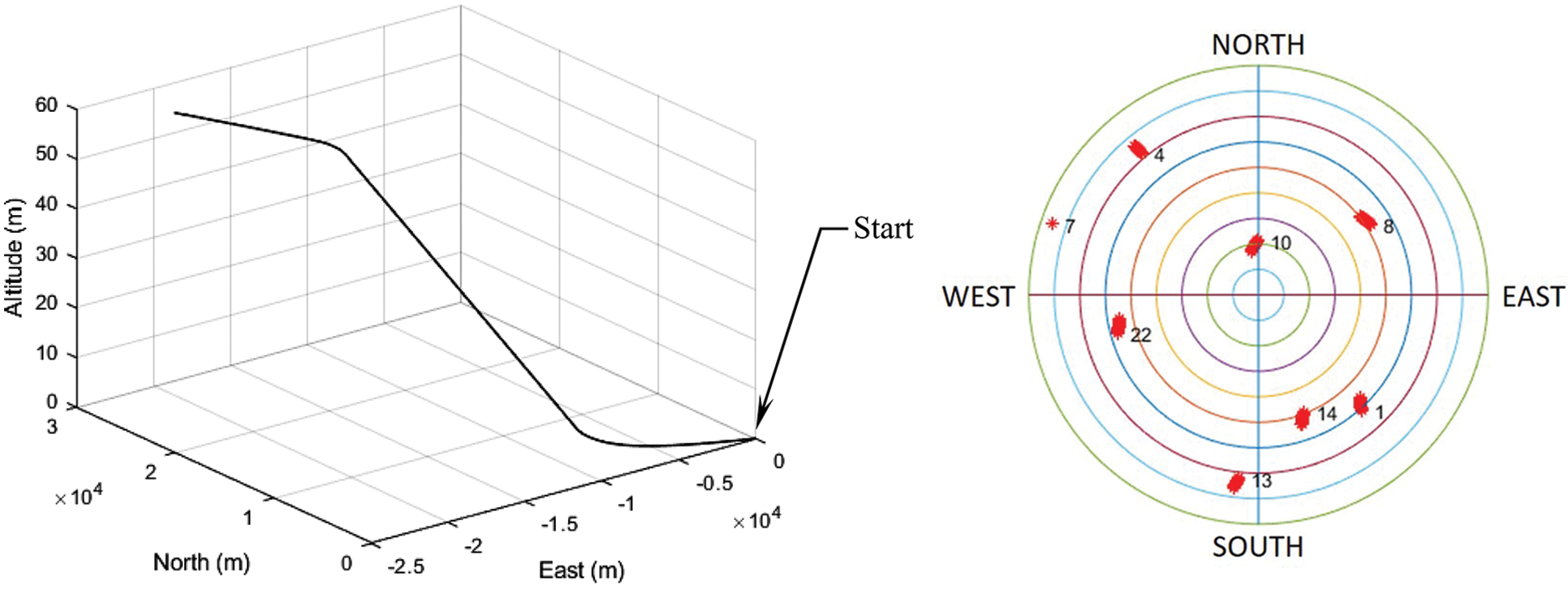
Figure 1: Test trajectory for the simulated vehicle (left) and the skyplot (right) during the simulation

5.1 Scenario 1: Pseudorange Observable Involving Outlier Type of Multipath Errors

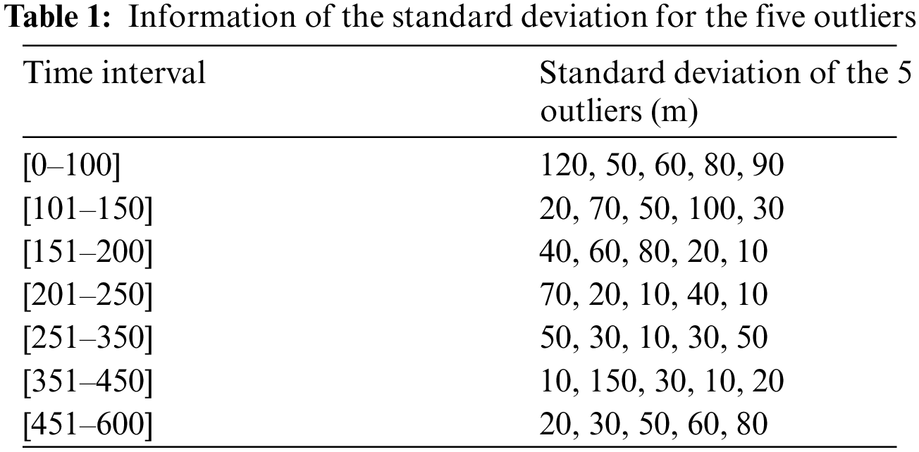
In Scenario 1, mitigation of the errors for pseudorange observable involving outlier type of multipath interferences is investigated. There are totally seven time durations where additional randomly generated errors are intentionally injected into the GPS pseudorange observation data during the vehicle moving. Tab. 1 provides the information of the standard deviation for the 5 outliers.

5.1.1 Performance Comparison for EKF and its Variants

Comparison of GPS navigation accuracy for the four schemes: EKF, VBEKF, HEKF and VBHEKF is shown in Fig. 2. The results show that either the VB or Huber's algorithms can assist EKF to effectively deal with the outliers in the pesudorange observables individually and combination of the two algorithms can furtherly enhance the performance.

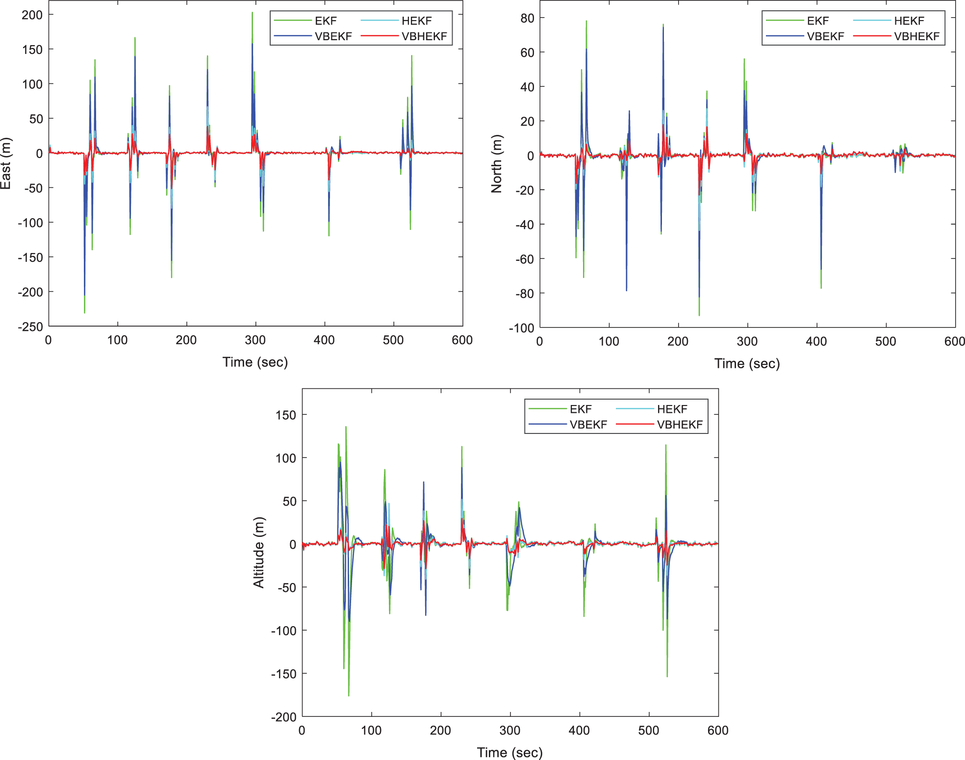
Figure 2: Comparison of positioning accuracy for extended Kalman filter (EKF) and its variants-Scenario 1

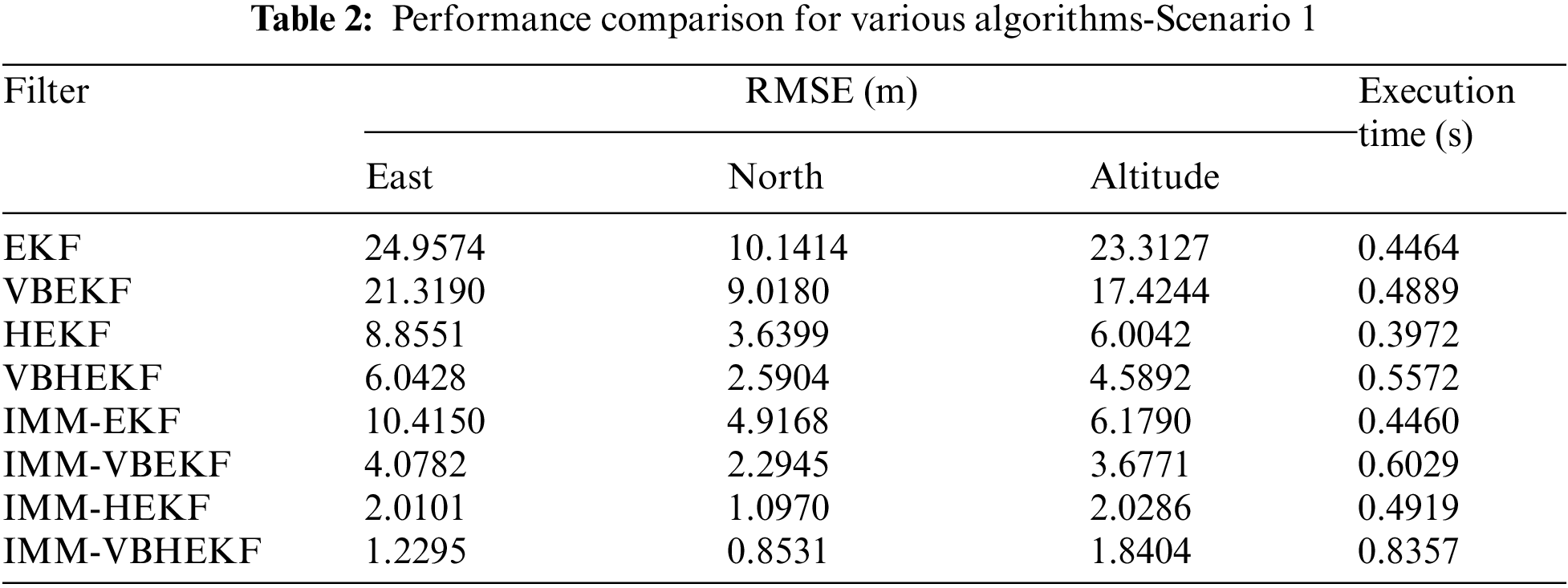
5.1.2 Performance Enhancement Based on the Interacting Multiple Model Configuration

Incorporation of the IMM into the various filters is utilized for further performance enhancement. Fig. 3 illustrates the positioning accuracy when the IMM configuration is involved for various algorithms: IMM-EKF, IMM-VBEKF, IMM-HEKF and IMM-VBHEKF. For the case that the VB does not possess sufficient capability to resolve the outlier type of interference, the IMM-VBHEKF demonstrates substantial performance improvement in navigation accuracy with acceptable extra computational expense. Tab. 2 summarizes the estimation performance and execution time for various algorithms.

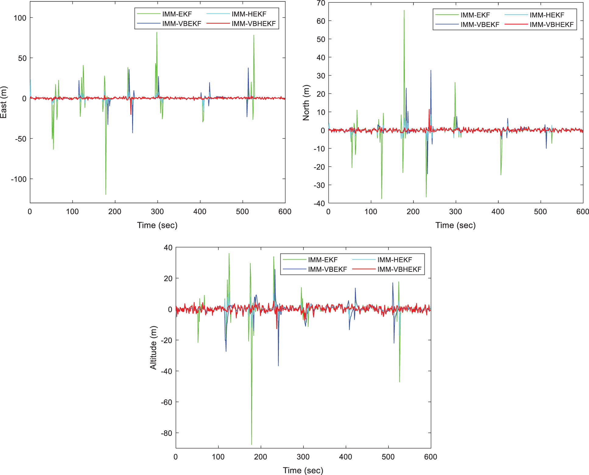
Figure 3: Comparison of positioning accuracy when the interacting multiple model (IMM) configuration is involved for Scenario 1

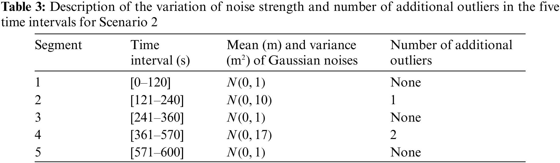
5.2 Scenario 2: Errors Involving Time-Varying Variance in Measurement Noise with Additional Outliers

Scenario 2 is designed for investigating the performance when dealing with the time-varying Gaussian measurement noise with additional outliers. Description of time varying measurement variances in the five time intervals is shown in Tab. 3. The variances of time-varying measurement noise rρi in the five time intervals for this scenario are assumed to follows the variation: rρi=1→10→1→17→1 (in unit of m2), where the ‘arrows (→)’ is employed for indicating the time-varying trajectory of variances. The set of unknown time-varying statistical parameters of noise needs to be estimated with the system states and the error covariance.

5.2.1 Performance Comparison for EKF and its Variants

Comparison of GPS navigation accuracy for the EKF, VBEKF, HEKF and VBHEKF is shown in Fig. 4 where comparison of positioning accuracies without outlier and with outlier, respectively is provided. The results show that both VB and Huber based EKF can effectively improve the positioning performance. As can be seen, both the VB and Huber algorithms can be adopted into the EKF to improve GPS navigation accuracy in the environment of time-varying Gaussian noise. When additional outliers are involved in addition to the time-varying interferences, neither VB nor Huber only algorithm possesses sufficient capability to resolve the problem for such kind of challenge. The VBHEKF demonstrates substantial performance improvement in navigation accuracy at the expense of acceptable extra computational cost.

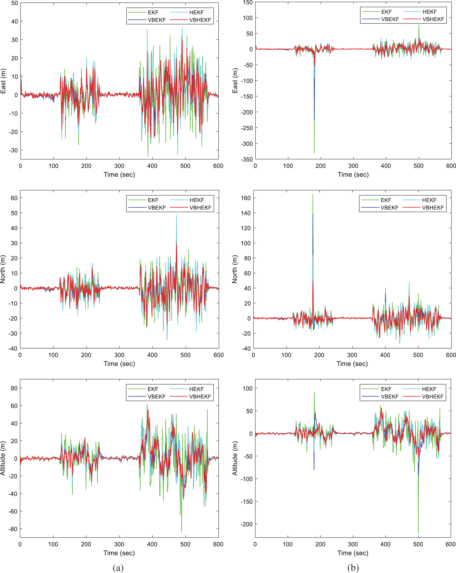
Figure 4: Comparison of positioning accuracy for EKF and its variants-Scenario 2 (a) without outlier (b) with outlier

5.2.2 Performance Enhancement Based on the Interacting Multiple Model Configuration

Comparison of positioning accuracies for the four algorithms: IMM-EKF, IMM-VBEKF, IMM-HEKF and IMM-VBHEKF is shown in Fig. 5. Positioning accuracies for the cases without and with outliers, respectively, are presented. The Huber's approach does not catch up the variation of noise strength very well. With the assistance of VB, the VBHEKF can further improve the performance. From the other view point, the adaptation capability of noise variance for the VBHEKF has been improved with the assistance of the IMM mechanism. Tabs. 4 and 5 summarize the performance for various algorithms without and with outliers, respectively. Among the various approaches, the IMM-VBHEKF provides the best positioning accuracy with only limited amount of extra execution time.

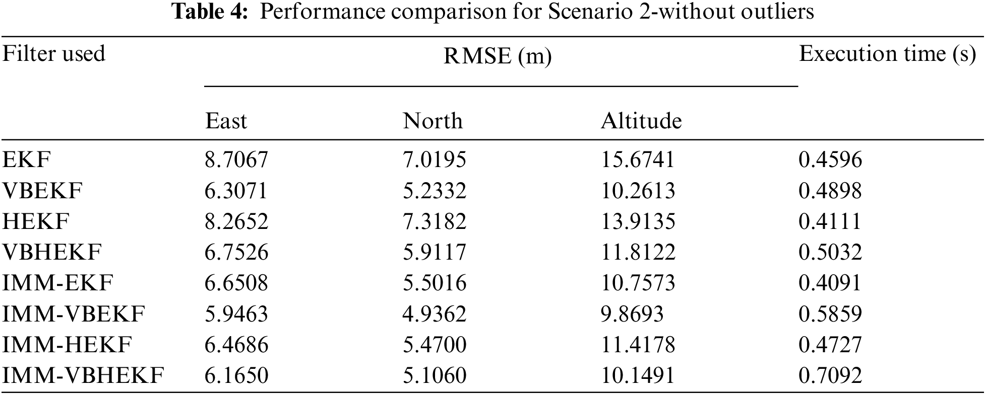
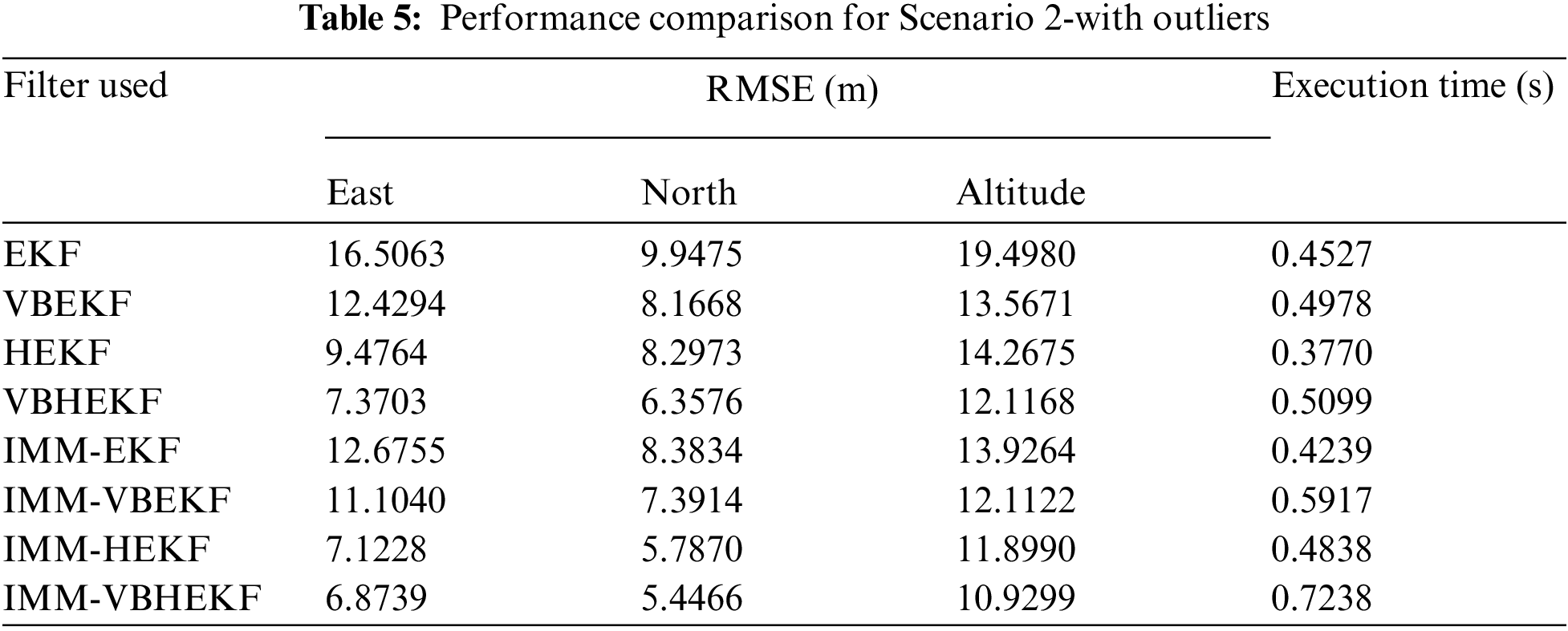
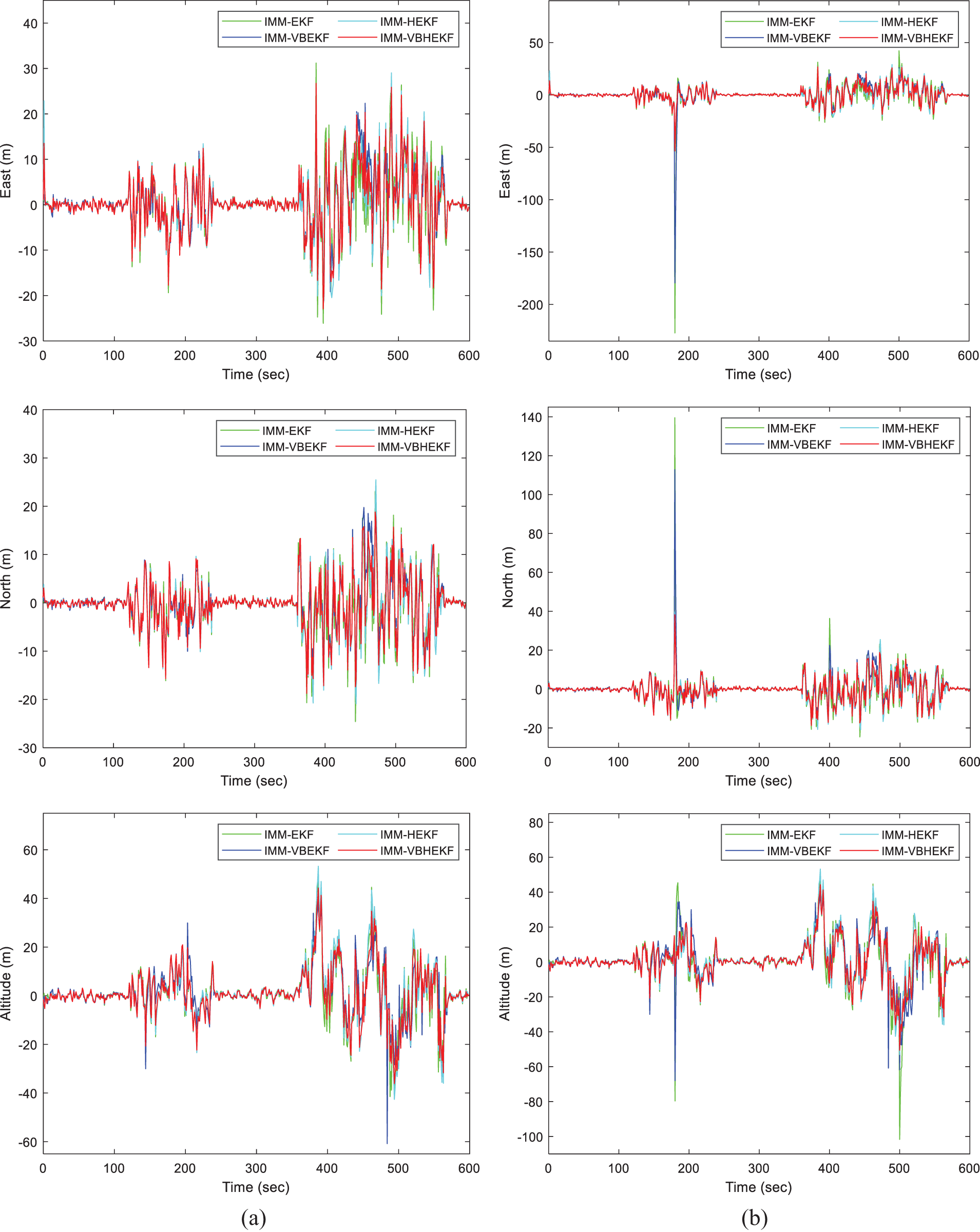
Figure 5: Comparison of positioning accuracy for Scenario 2 when the IMM configuration is involved when IMM algorithm is incorporated (a) without outlier (b) with outlier

6  Conclusions

In this paper, an interacting multiple model based variational Bayesian robust extended Kalman filter is adopted for processing GPS navigation states. The method utilizes the variational Bayesian learning to approximate the noise strength and to provide a strong tracking capability for time-varying noise covariances; the Huber M-estimation methodology based on the robust strategy is employed to enhance robustness especially for overcoming the problem of contamination distribution or outliers; the IMM algorithm is introduced for further tuning of the noise covariance matrices. Combination the three merits leads to the estimator referred to as the IMM-VBHEKF. Illustrative examples have been provided for validation of the method. Two scenarios are presented representing two possible peudorange error patterns, including (1) observable involving outlier type of multipath errors; (2) observable involving time-varying variance in measurement noise with additional outliers. The proposed method has demonstrated performance enhancement in terms of adaptivity and robustness at the expense of acceptable additional execution time.

Funding Statement: This work has been partially supported by the Ministry of Science and Technology, Taiwan [Grant Numbers MOST 108-2221-E-019-013 and MOST 109-2221-E-019-010].

Conflicts of Interest: The authors declare that they have no conflicts of interest to report regarding the present study.

References

 1.  B. Hofmann-Wellenhof, H. Lichtenegger and E. Wasle, GNSS–Global Navigation Satellite Systems, GPS, GLONASS, Galileo, and More, New York, NY, USA: Springer, 2008. [Google Scholar]

 2.  E. D. Kaplan and C. J. Hegarty, Understanding GPS: Principles and Applications, Norwood, MA, USA: Artech House, Inc., 2006. [Google Scholar]

 3.  T. Zhou, B. Lian, S. Yang, Y. Zhang and Y. Liu, “Improved GNSS cooperation positioning algorithm for indoor localization,” Computers, Materials & Continua, vol. 56, no. 2, pp. 225–245, 2018. [Google Scholar]

 4.  N. L. Knight and J. Wang, “A comparison of outlier detection procedures and robust estimation methods in GPS positioning,” The Journal of Navigation, vol. 62, no. 4, pp. 699–709, 2009. [Google Scholar]

 5.  R. G. Brown and P. Y. C. Hwang, Introduction to Random Signals and Applied Kalman Filtering, New York, NY, USA: John Wiley & Sons, 1997. [Google Scholar]

 6.  J. Wang and J. Wang, “Mitigating the effect of multiple outliers on GNSS navigation with M-estimation schemes,” in Proc. Int. Global Navigation Satellite Systems Society (IGNSS) Symposium, Sydney, Australia, 2007. [Google Scholar]

 7.  P. J. Huber, Robust Statistics, New York, NY, USA: Wiley, 1981. [Google Scholar]

 8.  X. Wang, N. Cui and J. Guo, “Huber-based unscented filtering and its application to vision-based relative navigation,” IET Radar Sonar Navigation, vol. 4, no. 1, pp. 134–141, 2010. [Google Scholar]

 9.  C. D. Karlgaard and H. Schaub, “Huber-based divided difference filtering,” Journal of Guidance, Control and Dynamics, vol. 30, no. 3, pp. 885–891, 2007. [Google Scholar]

10. S. Särkkä and A. Nummenmaa, “Recursive noise adaptive Kalman filtering by variational Bayesian approximations,” IEEE Transactions on Automatic Control, vol. 54, no. 3, pp. 596–600, 2009. [Google Scholar]

11. S. Särkkä and J. Hartikainen, “Nonlinear noise adaptive Kalman filtering via variational Bayes,” in Proc. IEEE Int. Workshop on Machine Learning for Signal Processing Southampton, UK, pp. 1–6, 2013. [Google Scholar]

12. P. Dong, Z. Jing, H. Leung and K. Shen, “Variational Bayesian adaptive cubature information filter based on wishart distribution,” IEEE Transactions on Automatic Control, vol. 62, no. 11, pp. 6051–6057, 2017. [Google Scholar]

13. K. Li, L. Chang and B. Hu, “A variational Bayesian-based unscented Kalman filter with both adaptivity and robustness,” IEEE Sensors Journal, vol. 16, no. 18, pp. 6966–6976, 2016. [Google Scholar]

14. Q. Wang and J. Huang, “A VB-IMM filter for ADS-B data,” in Proc. 2014 12th Int. Conf. on Signal Processing (ICSP), Hangzhou, China, pp. 2130–2134, 2014. [Google Scholar]

15. Y. Peng, W. Panlong and H. Shan, “An IMM-VB algorithm for hypersonic vehicle tracking with heavy tailed measurement noise,” in Proc. 2018 Int. Conf. on Control, Automation and Information Sciences (ICCAIS), Hangzhou, China, pp. 169–174, 2018. [Google Scholar]

16. A. H. Mohamed and K. P. Schwarz, “Adaptive Kalman filtering for INS/GPS,” Journal of Geodesy, vol. 73, pp. 193–203, 1999. [Google Scholar]

17. G. Chen and M. Harigae, “Using IMM adaptive estimator in GPS positioning,” in Proc. the 40th SICE Annual Conf., Nagoya, Japan, pp. 25–27, 2001. [Google Scholar]

18. X. Lin, T. Kirubarajan, Y. Bar-Shalom and X. Li, “Enhanced accuracy GPS navigation using the interacting multiple model estimator,” in Proc. IEEE Aerospace Conf., Montana, CA, USA, vol. 4, pp. 1911–1923, 2001. [Google Scholar]

19. C. Zhang, C. Guo and D. Zhang, “Data fusion based on adaptive interacting multiple model for GPS/INS integrated navigation system,” Applied Sciences, vol. 8, no. 9, pp. 1682, 2018. [Google Scholar]

20. D. Li and J. Sun, “Robust interacting multiple model filter based on student's t-distribution for heavy-tailed measurement noises,” Sensors, vol. 19, no. 22, pp. 4830, 2019. [Google Scholar]

21. D. Li, X. Ji and J. Zhao, “A novel hybrid fusion algorithm for low-cost GPS/INS integrated navigation system during GPS outages,” IEEE Access, vol. 8, pp. 53984–53996, 2020. [Google Scholar]

22. GPSoft LLC, Satellite Navigation Toolbox 3.0 User's Guide. Athens, OH, USA, 2003. [Google Scholar]

This work is licensed under a Creative Commons Attribution 4.0 International License, which permits unrestricted use, distribution, and reproduction in any medium, provided the original work is properly cited.