DOI:10.32604/cmc.2022.025118
| Computers, Materials & Continua DOI:10.32604/cmc.2022.025118 | |
| Article |
A New Method for Scene Classification from the Remote Sensing Images
1Department of CSE, B V Raju Institute of Technology, Narsapur, Medak, Telangana, India
2Department of Information Technology, College of Computers and Information Technology, Taif University, Taif, 21944, Saudi Arabia
3Department of Electronics and Communications, DVR&DHS MIC Engineering College, Kanchikacharla, Vijayawada, A.P., India
4Department of Computer Science, College of Computer and Information Systems, Umm Al-Qura University, Makkah, 21955, Saudi Arabia
5Department of ECE, P.V.P Siddhartha Institute of Technology, Vijayawada, India
6Department of Computer Science, College of Computers and Information Technology, Taif University, Taif, 21944, Saudi Arabia
*Corresponding Author: Neenavath Veeraiah. Email: neenavathveeru@gmail.com
Received: 12 November 2021; Accepted: 06 January 2022
Abstract: The mission of classifying remote sensing pictures based on their contents has a range of applications in a variety of areas. In recent years, a lot of interest has been generated in researching remote sensing image scene classification. Remote sensing image scene retrieval, and scene-driven remote sensing image object identification are included in the Remote sensing image scene understanding (RSISU) research. In the last several years, the number of deep learning (DL) methods that have emerged has caused the creation of new approaches to remote sensing image classification to gain major breakthroughs, providing new research and development possibilities for RS image classification. A new network called Pass Over (POEP) is proposed that utilizes both feature learning and end-to-end learning to solve the problem of picture scene comprehension using remote sensing imagery (RSISU). This article presents a method that combines feature fusion and extraction methods with classification algorithms for remote sensing for scene categorization. The benefits (POEP) include two advantages. The multi-resolution feature mapping is done first, using the POEP connections, and combines the several resolution-specific feature maps generated by the CNN, resulting in critical advantages for addressing the variation in RSISU data sets. Secondly, we are able to use Enhanced pooling to make the most use of the multi-resolution feature maps that include second-order information. This enables CNNs to better cope with (RSISU) issues by providing more representative feature learning. The data for this paper is stored in a UCI dataset with 21 types of pictures. In the beginning, the picture was pre-processed, then the features were retrieved using RESNET-50, Alexnet, and VGG-16 integration of architectures. After characteristics have been amalgamated and sent to the attention layer, after this characteristic has been fused, the process of classifying the data will take place. We utilize an ensemble classifier in our classification algorithm that utilizes the architecture of a Decision Tree and a Random Forest. Once the optimum findings have been found via performance analysis and comparison analysis.
Keywords: Remote sensing; RSISU; DL; RESNET-50; VGG-16
Information obtained through remote sensing, which provides us with important data about the Earth's surface, may enable us to precisely measure and monitor geographical features [1]. The rate of growth in the number of remote sensing pictures is due to the recent improvements in earth observation technologies. The urgency associated with the search for ways to make full use of expanding remote sensing pictures for intelligent earth observation has been heightened due to this. Thus, to make sense of large and complicated remote sensing pictures, it is crucial to comprehend them completely. In regard to their work as a difficult and difficult-to-solve issue for understanding remote sensing data, research on scene categorization [2,3] of remote sensing pictures has been quite active. Correctly labelling remote sensing pictures using pre-set semantic categories, as illustrated in Fig. 1, is a function of remote sensing image classification. Advanced remote sensing picture scene classification [4] research, which includes many studies on urban planning, natural hazards identification, environment monitoring, vegetation mapping, and geospatial item recognition, has occurred due to the significance of these fields in the real world [5,6].
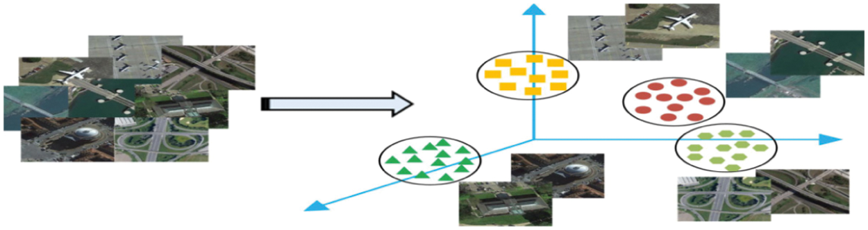
Figure 1: Classifying remote sensing imagery
Assigning a specific semantic name to a scene, such as “urban” and “forest,” is an example of the categorization of land-use scenes. An increase in satellite sensor development is enabling a massive rise in the amount of high-resolution remote sensing picture data. In order to create intelligent databases, it is essential to use robust and efficient categorization techniques on huge remote sensing pictures. Classifying aerial or satellite pictures using computer vision methods is very interesting. For example, the bag-of-visual-words (BOVW) paradigm groups the local visual characteristics collected from a series of pictures and creates a set of visual words (i.e., a visual vocabulary). A histogram shows how many words from a certain picture appear in the histogram. An acronym for Remote Sensing Land-Use Scene Categorization (BOVW) has been useful in classification of remote sensing images of land-use scenes, which have been a particularly excellent use of the BOVW model. However, this is ignoring the spatial information in the pictures. By integrating texture information into remote sensing land-use picture data, the BOVW model's performance may be enhanced. Fig. 2 shows the development of remote sensing picture classification by a progression from pixel-level, object-level, to scene-level categorization. Due to the variety of remote sensing picture classification systems, we choose to use the generic phrase of “remote sensing image classification” rather than “remote sensing image classification technology.” In general, scholars worked to categorize remote sensing pictures by labelling each pixel with a semantic class since the spatial resolution of remote sensing images is extremely poor, which is comparable to how things are represented in the early scientific literatures. Furthermore, this is still an ongoing research subject for multispectral and hyperspectral remote sensing picture analysis.
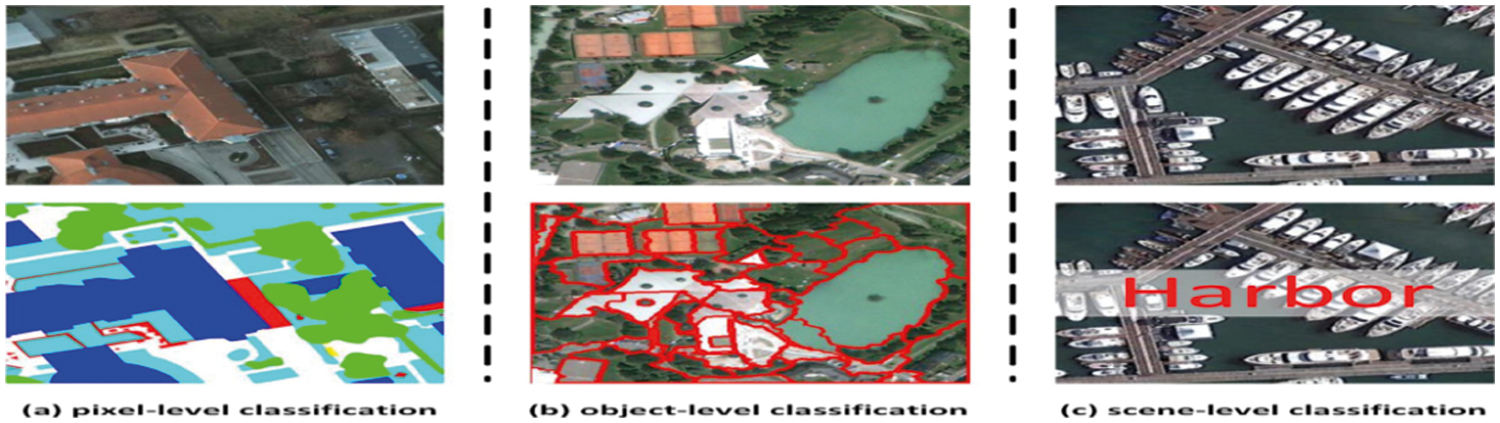
Figure 2: Classification of remote sensing images on three different levels
Computational time and memory utilization have become important advancements in computer vision. Classifiers, on the other hand, are needed to have significant generalization ability while also producing high performance. A growing area of study for remote sensing imagery characterization is noted. Extra remote sensing image analysis execution measures have been found using the feature-based method, which is an additional step from data mining strategies. Classification of images is an important use of computer vision in this field. Our main goal is to advance machine learning methods for remote sensing picture categorization. The information included in satellite pictures, such as buildings, landscapes, deserts, and structures, is categorized and analysed throughout time using images including satellite imagery [7].
This paper presents a method that combines feature fusion and extraction with classification algorithms for remote sensing for scene categorization. The benefits the benefits (POEP) include two advantages include two advantages. The multi-resolution feature mapping is done first, using the Pass Over connections, and combines the several resolution-specific feature maps generated by the CNN, resulting in critical advantages for addressing the variation in RSISU data sets. Secondly, we are able to use Enhanced pooling to make the most use of the multi-resolution feature maps that include second-order information. This enables CNNs to better cope with (RSISU) issues by providing more representative feature learning. In the beginning, the picture was pre-processed, then the features were retrieved using RESNET-50, Alexnet, and VGG-16 integration of architectures. After characteristics have been amalgamated and sent to the attention layer, after this characteristic has been fused, the process of classifying the data will take place. We utilize an ensemble classifier in our classification algorithm that utilizes the architecture of a Decision Tree and a Random Forest. Once the optimum findings have been found via performance analysis and comparison analysis.
The remainder of the article is structured as follows: Section 2 presents relevant literature on categories that have been observed. Section 3 outlines the proposed process. Section 4 presents the results. Summaries of conclusions is found in Section 5.
There are just a few iterations required for the RSSCNet model recommended by Sheng-Chieh et al. [8] to be used in conjunction with a two-stage cycle of learning rate training policy and the no-freezing transfer learning technology. It is possible to get a high degree of precision in this manner. Using data augmentation, regularization, and an early-stopping approach, the issue of restricted generalization observed during fast deep neural network training may be addressed as well. Using the model and training methods presented in this article outperforms existing models in terms of accuracy, according to the findings of the experiments. To be effective, this approach must concentrate on picture rectification pre-processing for cases where outliers are suspected and combine various explainable artificial intelligence analysis technologies to enhance interpretation skills. Kim et al. [9] proposed a new self-attention feature selection module integrated multi-scale feature fusion network for few-shot remote sensing scene categorization, referred to as SAFFNet. For a few-shot remote sensing classification task, informative representations of images with different receptive fields are automatically selected and re-weighted for feature fusion after refining network and global pooling operations. This is in contrast to a pyramidal feature hierarchy used for object detection. The support set in the few-shot learning job may be used to fine-tune the feature weighting value. The proposed remote sensing scene categorization model is tested on three public ally accessible datasets. To accomplish more efficient and meaningful training for the fine-tuning of a CNN backbone network, SAFFNet needs less unseen training samples.
The fusion-based approach for remote sensing picture scene categorization was suggested by Yin et al. [10] Front side fusion, middle side fusion, and rear side fusion are the three kinds of fusion modes that are specified. Different fusion modes have typical techniques. There are many experiments being conducted in their entirety. Various fusion mode combinations are tested. On widely used datasets, model accuracy and training efficiency results are shown. Random crop + numerous backbone + average is the most effective technique, as shown by the results of this experiment. Different fusion modes and their interactions are studied for their characteristics. Research on the fusion-based approach with particular structure must be conducted in detail, and an external dataset should be utilized to enhance model performance. Campos-Taberner et al. [11] using Sentinel-2 time data, this research seeks to better comprehend a recurrent neural network for land use categorization in the European Common Agricultural Policy setting (CAP). Using predictors to better understand network activity allows us to better address the significance of predictors throughout the categorization process. According to the results of the study, Sentinel-2's red and near infrared bands contain the most relevant data. The characteristics obtained from summer acquisitions were the most significant in terms of temporal information. These findings add to the knowledge of decision-making models used in the CAP to carry out the European Green Deal (EGD) intended to combat climate change, preserve biodiversity and ecosystems, and guarantee a fair economic return for farmers. They also help. This approach should put more emphasis on making accurate predictions.
An improved land categorization technique combining Recurrent Neural Networks (RNNs) and Random Forests (RFs) has been proposed for different research objectives by Xu et al. [12]. We made use of satellite image spatial data (i.e., time series). Pixel and object-based categorization are the foundations of our experimental classification. Analyses have shown that this new approach to remote sensing scene categorization beats the alternatives now available by up to 87%, according to the results. This approach should concentrate on the real-time use of big, complicated picture scene categorization data. For small sample sizes with deep feature fusion, a new sparse representation-based approach is suggested by Mei et al. [13]. To take full use of CNNs’ feature learning capabilities, multilevel features are first retrieved from various levels of CNNs. Observe how to extract features without labeled samples using current well-trained CNNs, e.g., AlexNet, VGGNet, and ResNet50. The multilevel features are then combined using sparse representation-based classification, which is particularly useful when there are only a limited number of training examples available. This approach outperforms several current methods, particularly when trained on small datasets as those from UC-Merced and WHU-RS19. For the categorization of remote sensing high-resolution pictures, Petrovska et al. [14] developed the two-stream concatenation technique. Aerial images were first processed using neural networks pre-trained on ImageNet datasets, which were then combined into a final picture using convolutional neural networks (CNNs). After the extraction, a convolutional layer's PCA transformed features and the average pooling layer's retrieved features were concatenated to create a unique feature representation. In the end, we classified the final set of characteristics using an SVM classifier. We put our design to the test using two different sets of data. Our architecture's outcomes were similar to those of other cutting-edge approaches. If a classifier has to be trained with a tiny ratio on the training dataset, the suggested approach may be useful. The UC-Merced dataset's “dense residential” picture class, for example, has a high degree of inter-class similarity, and this approach may be an effective option for classifying such datasets. The correctness of this procedure must be the primary concern.
End-to-end local-global-fusion feature extraction (LGFFE) network for more discriminative feature representation proposed by Lv and colleagues [15]. A high-level feature map derived from deep CNNs is used to extract global and local features from the channel and spatial dimensions, respectively. To capture spatial layout and context information across various areas, a new recurrent neural network (RNN)-based attention module is initially suggested for local characteristics. The relevant weight of each area is subsequently generated using gated recurrent units (GRUs), which take a series of image patch characteristics as input. By concentrating on the most important area, a rebalanced regional feature representation may be produced. By combining local and global features, the final feature representation will be obtained. End-to-end training is possible for feature extraction and feature fusion. However, this approach has the disadvantage of increasing the risk of misclassification due to a concentration on smaller geographic areas Hong et al. [16] suggest the use of CTFCNN, a CaffeNet-based technique for investigating a pre-trained CNN's discriminating abilities effectively. In the beginning, the pretrained CNN model is used as a feature extractor to acquire convolutional features from several layers, FC features, and FC features based on local binary patterns (LBPs). The discriminating information from each convolutional layer is then represented using an improved bag-of-view-word (iBoVW) coding technique. Finally, various characteristics are combined forcategorization using weighted concatenation. The proposed CTFCNN technique outperforms certain state-of-the-art algorithms on the UC-Merced dataset and the Aerial Image Dataset (AID), with overall accuracy up to 98.44% and 94.91%, respectively. This shows that the suggested framework is capable of describing the HSRRS picture in a specific way. The categorization performance of this technique need improvement. When generating discriminative hyperspectral pictures, Ahmed and colleagues [17] stressed the significance of spectral sensitivities. Such a representation's primary objective is to enhance picture content identification via the use of just the most relevant spectral channels during processing. The fundamental assumption is that each image's information can be better retrieved using a particular set of spectral sensitivity functions for a certain category. Content-Based Image Retrieval (CBIR) evaluates these spectral sensitivity functions. Specifically for Hyperspectral remote sensing retrieval and classification, we provide a new HSI dataset for the remote sensing community in this study. This dataset and a literature dataset have both been subjected to a slew of tests. Findings show that the HSI provides a more accurate representation of picture content than the RGB image presentation because of its physical measurements and optical characteristics. As the complexity of sensitivity functions increases, this approach should be refined. By considering existing methods drawbacks, we propose the Pass Over network for remote sensing scene categorization, a novel Hybrid Feature learning and end-to-end learning model that combines feature fusion and extraction with classification algorithms for remote sensing for scene categorization. In the beginning, the picture was pre-processed, then the features were retrieved using RESNET-50, Alexnet, and VGG-16 integration of architectures. After characteristics have been amalgamated and sent to the attention layer, after this characteristic has been fused, the process of classifying the data will take place. We utilize an ensemble classifier in our classification algorithm that utilizes the architecture of a Decision Tree and a Random Forest. Once the optimum findings have been found via performance analysis and comparison analysis.
The suggested network is part of the Hybrid Feature Learning [18] and End-to-End Learning Model Learning Systems category of networks. Proposed technique may be taught end-to-end, which improves classification performance compared to existing feature-based or feature learning-based approaches. Categorize the VGG-16, Alexnet, and Resnet-50 convolutions as Conv2D_3, Conv2D_4 and Conv2D_5 of Alexnet with the VGG-16 Conv2D_3, Conv2D_4, Conv2D_5 and also with Resnet-50 Conv2D_3, Conv2D_4, Conv2D_5. Instead of doing picture pre-processing, the suggested approach eliminates it altogether [19,20]. The proposed approach has the advantage of requiring a considerably smaller number of training parameters and proposed network requires a tenth of the characteristics of its competitors. Because of the limited number of parameters needed by proposed method, we are more likely to avoid the overfitting issue when training a deep CNN model on relatively small data sets. This is a significant innovation. Fig. 3 depicts the entire architecture.
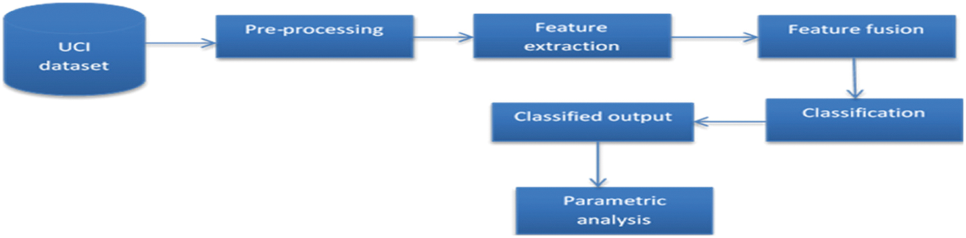
Figure 3: Overall architecture of proposed method
For remote sensing-based scene categorization, we developed an effective and efficient feature extraction approach using machine learning classifiers. The UCI dataset had 21 classes when it was first used. Dimensionality reduction [21,22] with noise removal has been used to pre-process this data. The extraction of features based on the architectures of RESNET-50, VGG-16, and Alexnet was then carried out. Based on the Multi-layer feature fusion model, this data has been merged (MFF). This was followed by a try at implementing the same action of focusing on just certain important items in the attention layer. The characteristics are then retrieved and categorized as a result of this procedure. Machine learning classifiers Randomn Forest [23] and Decision Tree were used to classify the retrieved feature. Fig. 4 depicts the suggested methodology's implementation architecture.
Pre-processing techniques for DR may take a variety of methods. In light of these benefits, the DR is taken into consideration. The amount of memory available for storing information decreases as the size of the object shrinks [24–26]. Fewer dimensions need shorter training and calculation durations. Most feature extraction techniques struggle when dealing with data that has many dimensions. DR methods effectively deal with the multi-collinearity of various data characteristics and remove redundancy within them. Finally, the data's smaller size makes it easier to see.
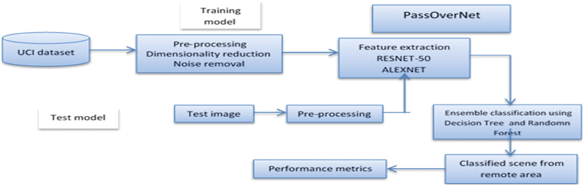
Figure 4: Architecture for implementing the suggested approach
3.1 Hybrid Feature Learning and End-to-End Learning Model
Fig. 5 depicts the proposed network's design, which makes use of the RESNET-50, VGG-16, and ALEXNET backbones. Three convolution layers are utilized to convolute the input, while the rest are skipped via Pass Over connections, as stated before. A matrix is formed along the channel dimension of the feature maps if the multi-resolution feature maps are designated as “X” instead of “X”. The resulting multi-resolution feature maps are then aggregated using a multi-scale pooling layer. The FC layer and SoftMax layer follow this one. Following that, we'll go through the two newest additions: Pass Over connections and multi-scale pooling.
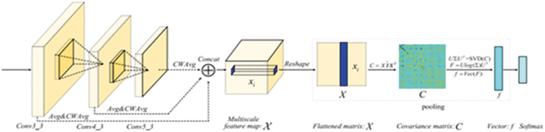
Figure 5: Architecture of the proposed POEP network
For illustrative purposes, the backbone consists of the off-the-shelf Resnet 50, Alexnet, and VGG-16. The Pass Over connection operation and a multi-scale pooling approach combine the feature maps from several layers. SVD refers to the singular value decomposition, whereas Vec indicates the vectorization process. Concat refers to the concatenate operation. CWAvg stands for channel-wise average pooling, whereas Avg indicates average pooling on the network as a whole. End-to-end learning system (also known as a hybrid system) is the classification given to the planned POEP network. Our methodology may be taught utilizing a hybrid feature learning and end-to-end learning strategy, which enhances classification performance in comparison to hand-crafted feature-based methods or feature learning-based techniques. It also exhibits competitive classification performance when compared to existing method. In comparison to other approaches, ours has the benefit of needing a much smaller set of training settings. The parameters needed by our POEP network's competitors are reduced by 90%. As a result of our methodology's fewer parameters, we're more likely to avoid overfitting problems while training a deep CNN model on a small data set. The Alexnet and Resnet-51 are used as Pass Over connections in the suggested approach [27–30].
3.2 Multi-Layer Aggregation Passover Connections
Let's say there are three sets of feature maps accessible, all with the same resolution.
In this case, [
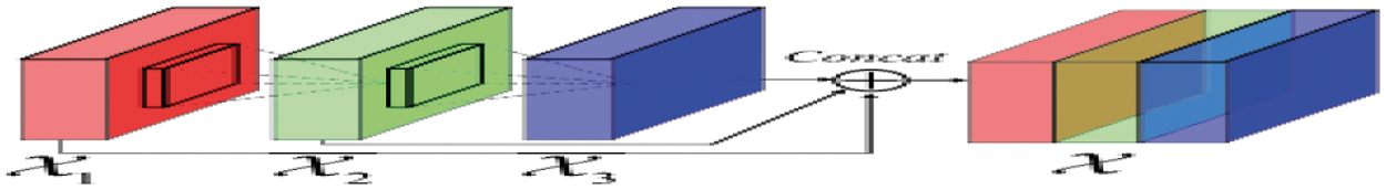
Figure 6: The feature map pass-through connections
Second, the data contained in the feature maps generated from different levels is complementary. Example of using feature maps from Alexnet's different layers for demonstration purposes is shown in Fig. 7. When using the Pass Over connection, you may take use of the feature maps’ diverse set of characteristics to improve classification precision
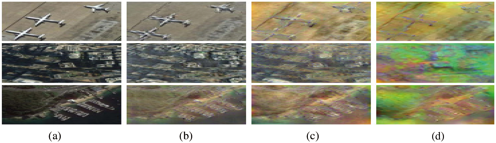
Figure 7: Graphical example illustrating the feature maps extracted from different layers of Alexnet for three different images. (a) Input image. (b) Feature map from the third convolutional layer. (c) Feature map from the fourth convolutional layer. (d) Feature map from the fifth convolutional layer
Note that average pooling is used to combine feature maps with varying spatial resolutions. Prior to concatenating the feature maps, CWAvg pooling is used to decrease the number of channels in each set by a factor of 2. The following is a comprehensive mathematical explanation of CWAvg pooling.
Consequently,
Forward Propagation of Multi-scale Pooling
The forward propagation of Multi-scale Pooling is performed as follows for a feature matrix
where
A matrix with the elements
Backward Propagation of Multi-scale Pooling
Multi-scale pooling uses global and structured matrix calculations instead of the conventional max or average pooling methods, which treat the intermediate variable's spatial coordinates (a matrix or a vector) separately. To calculate the partial derivative of the loss function L with respect to the multi-scale pooling input matrix, we use the matrix back-propagation technique. Because of this, we initially treat (∂ L/∂F), (∂ L/∂U) and (∂ L/∂
The fluctuation of the relevant variable is denoted by d(.). The: operation is represented by the symbol, and A: B = the trace (AT B). The following formulation may be derived from (5):
Putting (6) into (5), (∂ L/∂U) and (∂ L/∂) are obtained as follows:
To get (∂ L/∂U) and (∂ L/∂), let us compute (∂ L/∂C) through use the eigen decomposition (EIG) of C and C = UUT, and then calculate (L/C). The following is the whole chain rule expression:
Like (6), This version of matrix C may be obtained.
Eqs. (8) and (9) may be used with the characteristics of the matrix inner product, and the EIG properties to obtain the following partial derivatives of the loss function L relative to C
where ◦ denotes the Hadamard product, (⋅) sym denotes a symmetric operation, (⋅) diag is (⋅) with all off-diagonal elements being 0, and K is computed by manipulating the eigenvalues σ in as shown in the following:
There are further instructions on how to calculate (7) and (10). Lastly, (∂ L/∂C), assuming that the loss function L has a partial derivative with respect to the feature matrix X of the form:
3.3 Network Architecture for Proposed VGG-16
Tab. 1 lists the VGG-16's architectural specs. It has 3 FC layers and 5 3 × 3 convolutional layers, each having a stride size of 1. The stride for 2 × 2 pooling layers is 2, while the input picture size in VGG-16 is 224 × 224 by default. Every time a pooling layer is applied, the feature map is shrunk by a factor of two. FC layer features a 7 × 7 feature map with 512 channels that is expanded to a vector with 25,088 (7 × 7 × 512) channels before the FC layer is applied.
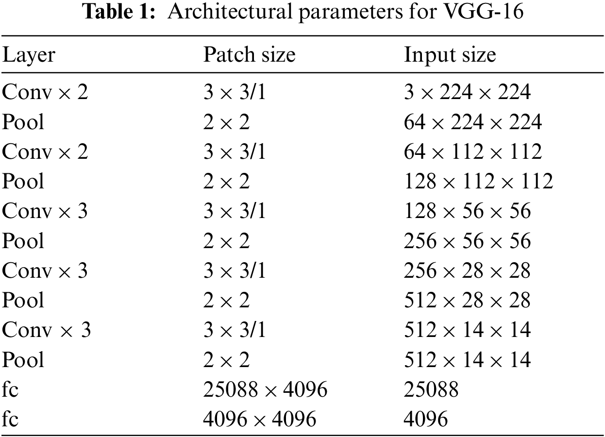
VGG-16 uses five convolutional layer blocks to process 224 × 224 video frame images. As the number of 3 × 3 filters increases, so does the complexity of the block. This is done using a stride of 1 while padding the convolutional layer's inputs to maintain spatial resolution. The max-pooling layers are used to disconnect every block. Stride 2 has 22 windows, which are used for max-pooling. Three FC layers are included in addition to the Convolutional layers. After that, the soft-max layer is applied, and here is where the class probabilities are calculated. The complete network model is shown in Fig. 8.
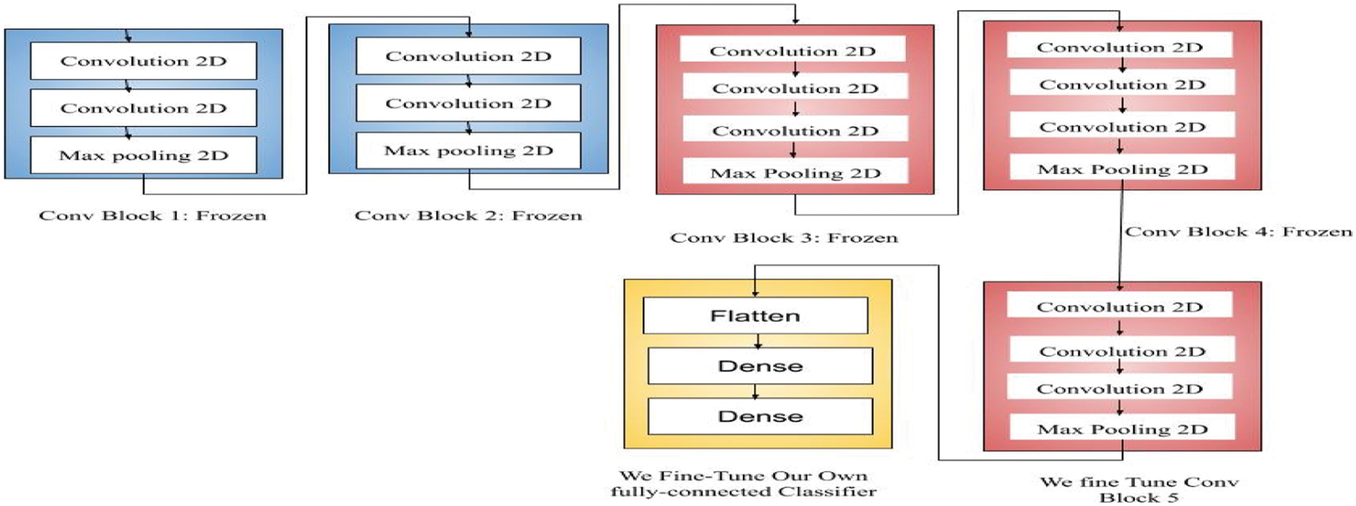
Figure 8: Network model for VGG-16
3.4 Ensemble Classifier [Random Forest and Decision Tree]
K basic decision trees are merged to create the random forest, which is a combined classifier. For the first batch of data, we used
From the original datasets randomly select sub-datasets
The random forest method generates K training subsets from the original dataset using the bagging sampling approach. Approximately two-thirds of the original dataset is used for each training subset, and samples are taken at random and then re-used in the sampling process. Every time in the sample set, the sample's chance of being acquired is 1/m, while the probability of not being obtained is (1 − 1/m). It isn't gathered after m samples are taken. The chances are. When m approaches infinity, the expression becomes
To put it another way, the Gini coefficient is a measure of the likelihood that a randomly chosen portion of a sample set will be divided in half. To put it another way, a smaller Gini index indicates that there is a lesser chance that the chosen sample will be divided, while a larger Gini index signifies that the collection is purer.
That is the Gini index (Gini impurity) = (probability of the sample being selected) * (probability of the sample being misclassified).
1. When the possibility that a sample belongs to the kth category is given by pk, the likelihood that the sample will be divided is given by (1 − pk).
2. Samples may belong to any of the K categories, and a random sample from the set can, too, thus increasing the number of categories.
3. When it's split into two, Gini(P) = 2p(1 − p)
If a feature is used to split a sample set into D1 and D2, there are only two sets: D1 equals the given feature value and D2 does not, in fact, contain the provided feature value. CART (classification and regression trees) are binary trees. Multiple values are binary processed in a single way.
To find out how pure each subset of the sample set D is, divide it into two using the partitioning feature = a certain feature value.
This means that when there are more than two values for a feature, the purity Gini(D, Ai) of the subset must be calculated after each value is divided by the sample D as the dividing point (where Ai represents the characteristic A Possible value) The lowest Gini index among all feasible Gini values is then determined (D, Ai). Based on the data in sample set D, this partition's division is the optimal division point.
3.5 Algorithm Description of the Random Forest
After the random sampling process, the resulting decision tree can be trained with data. According to the idea of random forests, decision trees have a high degree of independence from each other, and this feature also ensures the independence of the results produced by each decision tree. Then the remaining work consists of two: performing training tasks on each decision tree to produce results and voting to select the optimal solution from the results. Fig. 9 shows the tree.
Algorithm stages may be summed up by the following description:
Step1: This decision tree is made up of nodes that are randomly chosen from a large range of possible values for the dataset's characteristics, S. The number of s in the decision tree does not vary as the tree grows.
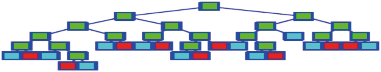
Figure 9: Classification tree topology
Step2: Uses the GINI technique to divide the node.
Step3: Set up a training environment for each decision tree and run training exercises
Step4: Vote to determine the optimal solution; Definition 1. for a group of classifiers
where I(•) is used as an indication. It's 1 if the equation in parentheses holds true; if not, it's 0.
The margin function measures how accurate the average categorization is compared to how inaccurate it is. The more reliable something is, the higher its worth.
The error message is as follows:
For a set of decision trees, all sequences Θ1, Θ2,….Θκ, The error will converge to
To prevent over-fitting, the random selection of the number of samples and the attribute may be utilized as described in the random forest approach.
As an example, there are 21 scene types in the UC Merced Land Use dataset: agri-industrial/aeronautical/baseballdiamond/beach/buildings/chaparral/freeway/forest/intersection/medium-residential/mobile-home-park/overpass/parkinglot/river/ruway/tennis-court There are 100 pictures in each class, each of which is 256 × 256 pixels in size.
Fig. 10 shows the Confusion matrix of the and the ROC Curve of Alexnet with the Decision tree classifier, Alexnet with the Random Forest classifier, Resnet-50 with the Decision tree classifier, Resnet-50 with the Random Forest classifier, VGG-16 with the Decision tree classifier and VGG-16 with the Random Forest classifier combinations for the 21 classes images of agricultural, airplane, beach, baseball diamond, buildings, chaparral, dense residential, forest freeway golf course, harbor, intersection, medium residential, mobile home park, over pass, parking lot, river Runway, sparse residential, storage tanks and tennis court are drawn between the True positivity rate to the False positivity rate.
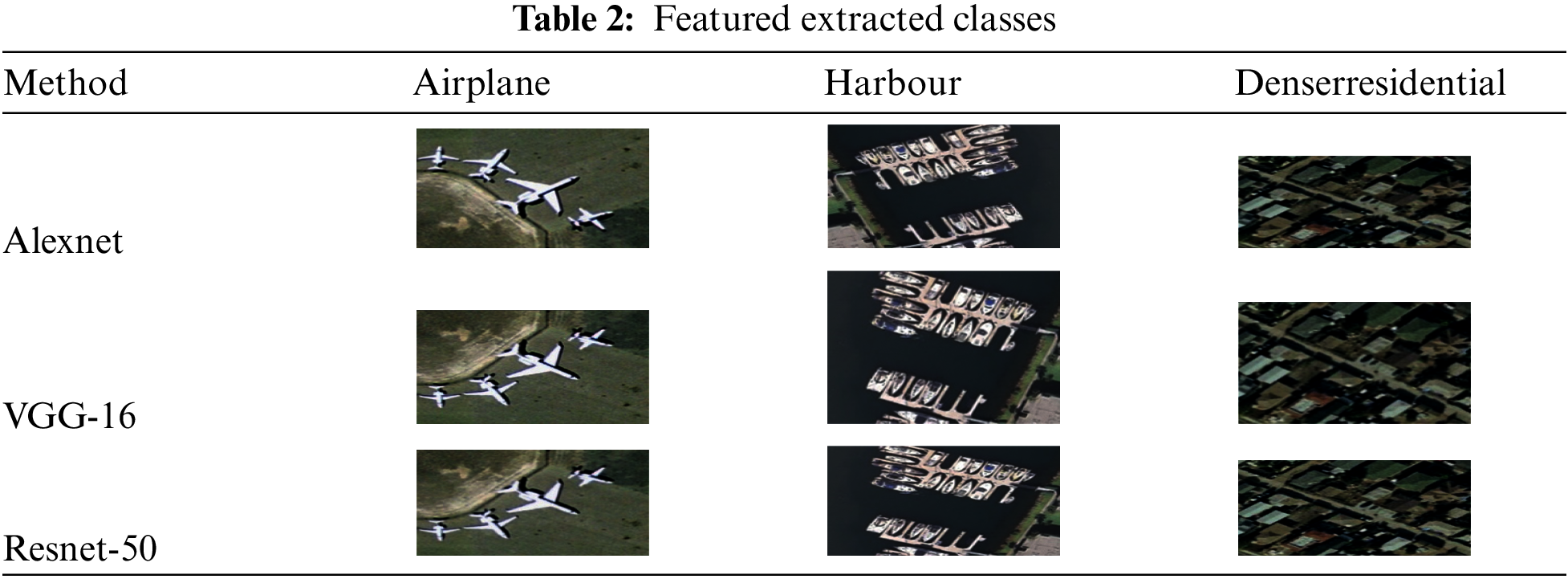
Tab. 2 shows how the featured extracted classes after the Concatenate the Conv2D_3, Conv2D_4 and Conv2D_5 of Alexnet with the VGG-16 Conv2D_3, Conv2D_4, Conv2D_5 and also with Resnet-50 Conv2D_3, Conv2D_4, Conv2D_5.
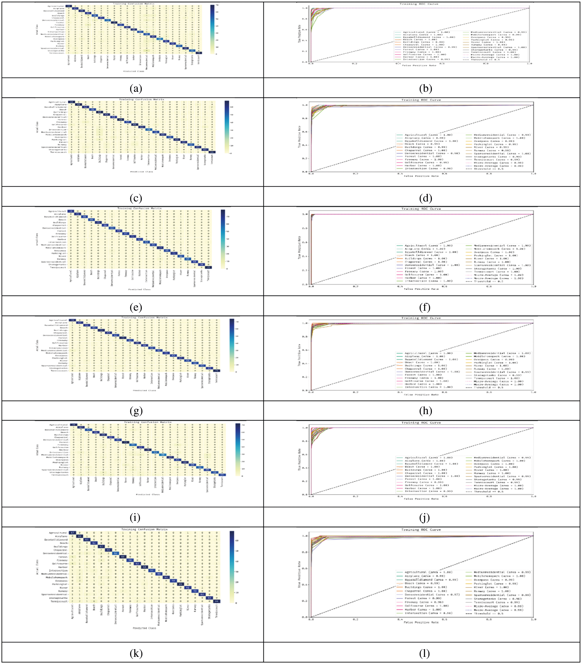
Figure 10: The confusion matrix and ROC curve for the 21 classes of (a) & (b) Alexnet with the decision tree classifier (c) & (d) Alexnet with the random forest classifier (e) & (f) Resnet-50 with the decision tree classifier (g) & (h) Resnet-50 with the random forest classifier (i) & (j) VGG-16 with the decision tree classifier (k) & (l) VGG-16 with the random forest classifier
It has been analysed that the input to the VGG-16, Resnet-50 and Alexnet the accuracy is less compared to the proposed model, the time consumption to train the existing is shown in Tab. 3.
ALEXNET -> {‘Training Time Per Epoch': 3.955 min, ‘Accuracy': 0.1895 (5 Epochs)}
VGG16 -> {‘Training Time Per Epoch': 6.22 min, ‘Accuracy': 0.0476 (1 Epoch)}

RESNET50 -> {‘Training Time Per Epoch': 10.185 min, ‘Accuracy': 0.0633} and the proposed Feature Extraction the time consumption is 52 min and the Classification time is 15 s. The accuracy model for the Alexnet [21] is about 90.21%, the accuracy level for the training model Resnet50 is about 62.01% for training and 91.85% for the VGG16 and the proposed architecture model gets the highest model of about 97.3%.
This paper proposes the Pass Over network for remote sensing scene categorization, a novel Hybrid Feature learning and end-to-end learning model. The Pass Over connection procedure, followed by a multi-scale pooling approach, introduces two new components, i.e., pass over connections and the feature maps from various levels. In addition to combining multi-resolution feature maps from various layers in the CNN model, our Pass Over network can also use high-order information to achieve more representative feature learning. It was found that the accuracy of the current ALEXNET, VGG16, RESNET50, and the proposed Feature Extraction is less than half that of the proposed model, and that the time required to train the existing models is 52 min longer than the proposed Feature Extraction's classification time. It's estimated that Alexnet's accuracy model is 90.21%, while Resnet50's training model accuracy level is 62.01%, while the VGG16 model accuracy is 91.85%, and the suggested architectural model obtains a high accuracy estimate of 97.3 percent.
Acknowledgement: We deeply acknowledge Taif University for supporting this study through Taif University Researchers Supporting Project Number (TURSP-2020/115), Taif University, Taif, Saudi Arabia.
Funding Statement: This research is funded by Taif University, TURSP-2020/115.
Conflicts of Interest: The authors declare that they have no conflicts of interest to report regarding the present study.
1. Y. Li, Y. Tan, L. Yi, S. Qi and J. Tian, “Built-up area detection from satellite images using multi kernel learning, multifield integrating, and multi hypothesis voting,” IEEE Geoscience and Remote Sensing Letters, vol. 12, no. 6, pp. 1190–1194, 2017. [Google Scholar]
2. K. Pradeep and N. Veeraiah, “VLSI implementation of euler number computation and stereo vision concept for cordic based image registration,” in Proc. 10th IEEE Int. Conf. on Communication Systems and Network Technologies (CSNT), Bhopal, India, pp. 269–272, 2021. [Google Scholar]
3. Y. Tan, S. Xiong and Y. Li, “Automatic extraction of built-up areas from panchromatic and multispectral remote sensing images using double-stream deep convolutional neural networks,” IEEE Journal of Selected Topics in Applied Earth Observations and Remote Sensing, vol. 11, no. 11, pp. 3988–4004, 2018. [Google Scholar]
4. D. Zhang, J. Han, C. Gong, Z. Liu, S. Bu et al.., “Weakly supervised learning for target detection in remote sensing images,” IEEE Geoscience and Remote Sensing Letters, vol. 12, no. 12, pp. 701–705, 2014. [Google Scholar]
5. Y. Li, Y. Zhang, X. Huang and A. L. Yuille, “Deep networks under scene-level supervision for multi-class geospatial object detection from remote sensing images,” ISPRS Journal of Photogrammetry and Remote Sensing, vol. 146, pp. 182–196, 2018. [Google Scholar]
6. W. Zhao and S. Du, “Learning multiscale and deep representations for classifying remotely sensed imagery,” ISPRS Journal of Photogrammetry and Remote Sensing, vol. 113, pp. 155–165, 2016. [Google Scholar]
7. O. A. B. Penatti, K. Nogueira and J. A. d Santos, “Do deep features generalize from everyday objects to remote sensing and aerial scenes domains,” in Proc. IEEE Conf. on Computer Vision and Pattern Recognition Workshops (CVPRW), Boston, MA, USA, pp. 44–51, 2015. [Google Scholar]
8. H. Sheng-Chieh, H. C. Wu and M. H. Tseng, “Remote sensing scene classification and explanation using RSSCNet and LIME,” Applied Sciences, vol. 10, no. 18, pp. 6151, 2020. [Google Scholar]
9. J. Kim and M. Chi, “SAFFNet-self-attention-based feature fusion network for remote sensing few-shot scene classification,” Remote Sensing, vol. 13, no. 13, pp. 2532, 2020. [Google Scholar]
10. L. Yin, P. Yang, K. Mao and Q. Liu, “Remote sensing image scene classification based on fusion method,” Journal of Sensors, vol. 2021, pp. 14, 2021. [Google Scholar]
11. M. Campos-Taberner, F. J. García-Haro, B. Martínez, E. Izquierdo-Verdiguier, C. Atzberger et al., “Understanding deep learning in land use classification based on sentinel-2 time series,” Scientific Reports, vol. 10, pp. 17188, 2020. [Google Scholar]
12. X. Xu, Y. Chen, J. Zhang, Y. Chen, P. Anandhan et al.., “A novel approach for scene classification from remote sensing images using deep learning methods,” European Journal of Remote Sensing, vol. 54, no. sup2, pp. 383–395, 2021. [Google Scholar]
13. S. Mei, K. Yan, M. Ma, X. Chen, S. Zhang et al., “Remote sensing scene classification using sparse representation-based framework with deep feature fusion,” IEEE Journal of Selected Topics in Applied Earth Observations and Remote Sensing, vol. 14, pp. 5867–5878, 2021. [Google Scholar]
14. B. Petrovska, E. Zdravevski, P. Lameski, R. Corizzo, I. Štajduhar et al., “Deep learning for feature extraction in remote sensing: A case-study of aerial scene classification,” Sensors, vol. 20, no. 14, pp. 3906, 2020. [Google Scholar]
15. Y. Lv, X. Zhang, W. Xiong, Y. Cui and M. Cai, “An end-to-end local-global-fusion feature extraction network for remote sensing image scene classification,” Remote Sensing, vol. 11, no. 24, pp. 3006, 2019. [Google Scholar]
16. H. Hong and K. Xu, “Combing triple-part features of convolutional neural networks for scene classification in remote sensing,” Remote Sensing, vol. 11, no. 14, pp. 1687, 2019. [Google Scholar]
17. O. B. Ahmed, T. Urruty, N. Richard and F. M. Christine, “Toward content-based hyperspectral remote sensing image retrieval (cb-hrsirA preliminary study based on spectral sensitivity functions,” Remote Sensing, vol. 11, no. 5, pp. 600, 2019. [Google Scholar]
18. R. Yun, C. Zhu and S. Xiao, “Small object detection in optical remote sensing images via modified faster r-cnn,” Applied Sciences, vol. 8, no. 5, pp. 813, 2018. [Google Scholar]
19. N. He, L. Fang, S. Li, J. Plaza and A. Plaza, “Skip-connected covariance network for remote sensing scene classification,” IEEE Transactions on Neural Networks and Learning Systems, vol. 31, no. 5, pp. 1461–1474, 2020. [Google Scholar]
20. B. Dai, R. C. Chen, S. Z. Zhu and W. W. Zhang, “Using random forest algorithm for breast cancer diagnosis,” 2018 International Symposium on Computer, Consumer and Control (IS3C), pp. 449–452, 2018. [Google Scholar]
21. D. Zeng, S. Chen, B. Chen and S. Li, “Improving remote sensing scene classification by integrating global-context and local-object features,” Remote Sensing, vol. 10, no. 5, pp. 1–19, 2018. [Google Scholar]
22. G. Suryanarayana, K. Chandran, O. I. Khalaf, Y. Alotaibi, A. Alsufyani et al., “Accurate magnetic resonance image super-resolution using deep networks and Gaussian filtering in the stationary wavelet domain,” IEEE Access, vol. 9, pp. 71406–71417, 2021. [Google Scholar]
23. X. Han, Y. Zhong, L. Cao and L. Zhang, “Pre-trained alexnet architecture with pyramid pooling and supervision for high spatial resolution remote sensing image scene classification,” Remote Sensing, vol. 9, pp. 848, 2017. [Google Scholar]
24. Y. Yao, H. Zhao, D. Huang and Q. Tan, “Remote sensing scene classification using multiple pyramid pooling,” International Archives of the Photogrammetry, Remote Sensing & Spatial Information Sciences, vol. XLII-2/W16, pp. 279–284, 2019. [Google Scholar]
25. P. Li, P. Ren, X. Zhang, Q. Wang, X. Zhu et al., “Region-wise deep feature representation for remote sensing images,” Remote Sensing, vol. 10, pp. 871, 2018. [Google Scholar]
26. N. Veeraiah, O. I. Khalaf, C. V. P. R. Prasad, Y. Alotaibi, A. Alsufyani et al., “Trust aware secure energy efficient hybrid protocol for manet,” IEEE Access, vol. 9, pp. 120996–121005, 2021. [Google Scholar]
27. A. Alsufyani, Y. Alotaibi, A. O. Almagrabi, S. A. Alghamdi and N. Alsufyani, “Optimized intelligent data management framework for a cyber-physical system for computational applications,” in Complex & Intelligent Systems, Springer, pp. 1–13, 2021. [Google Scholar]
28. Y. Alotaibi, M. N. Malik, H. H. Khan, A. Batool, ul Islam S. et al., “Suggestion mining from opinionated text of big social media data,” Computers, Materials & Continua, vol. 68, no. 3, pp. 3323–3338, 2021. [Google Scholar]
29. G. Li, F. Liu, A. Sharma, O. I. Khalaf, Y. Alotaibi et al., “Research on the natural language recognition method based on cluster analysis using neural network,” in Mathematical Problems in Engineering, Hindawi, vol. 2021, 2021. [Google Scholar]
30. Y. Alotaibi, “A new database intrusion detection approach based on hybrid meta-heuristics,” Computers, Materials & Continua, vol. 66, no. 2, pp. 1879–1895, 2021. [Google Scholar]
31. Y. Alotaibi, “Automated business process modelling for analyzing sustainable system requirements engineering,” in Proc. 6th Int. Conf. on Information Management (ICIM), London, UK, pp. 157–161, 2020. [Google Scholar]
32. A. Ma, Y. Wan, Y. Zhong, J. Wang and L. Zhang, “SCENE NET: Remote sensing scene classification deep learning network using multi-objective neural evolution architecture search,” ISPRS Journal of Photogrammetry and Remote Sensing, vol. 172, pp. 171–188, 2021. [Google Scholar]
33. X. Wu, Z. Zhang, W. Zhang, Y. Yi, C. Zhang et al., “A convolutional neural network based on grouping structure for scene classification,” Remote Sensing, vol. 13, no. 12, pp. 2457, 2021. [Google Scholar]
 | This work is licensed under a Creative Commons Attribution 4.0 International License, which permits unrestricted use, distribution, and reproduction in any medium, provided the original work is properly cited. |