Computers, Materials & Continua DOI:10.32604/cmc.2022.025550
Article

Intelligent Deep Data Analytics Based Remote Sensing Scene Classification Model

Ahmed Althobaiti1, Abdullah Alhumaidi Alotaibi2, Sayed Abdel-Khalek3, Suliman A. Alsuhibany4 and Romany F. Mansour5,*

1Department of Electrical Engineering, College of Engineering, Taif University, P.O. Box 11099, Taif, 21944, Saudi Arabia
2Department of Science and Technology, College of Ranyah, Taif University, P.O. Box 11099, Taif, 21944, Saudi Arabia
3Department of Mathematics, College of Science, P.O. Box 11099, Taif University, Taif, 21944, Saudi Arabia
4Department of Computer Science, College of Computer, Qassim University, Buraydah, 51452, Saudi Arabia
5Department of Mathematics, Faculty of Science, New Valley University, El-Kharga, 72511, Egypt
*Corresponding Author: Romany F. Mansour. Email: romanyf@sci.nvu.edu.eg
Received: 27 November 2021; Accepted: 11 January 2022

Abstract: Latest advancements in the integration of camera sensors paves a way for new Unmanned Aerial Vehicles (UAVs) applications such as analyzing geographical (spatial) variations of earth science in mitigating harmful environmental impacts and climate change. UAVs have achieved significant attention as a remote sensing environment, which captures high-resolution images from different scenes such as land, forest fire, flooding threats, road collision, landslides, and so on to enhance data analysis and decision making. Dynamic scene classification has attracted much attention in the examination of earth data captured by UAVs. This paper proposes a new multi-modal fusion based earth data classification (MMF-EDC) model. The MMF-EDC technique aims to identify the patterns that exist in the earth data and classifies them into appropriate class labels. The MMF-EDC technique involves a fusion of histogram of gradients (HOG), local binary patterns (LBP), and residual network (ResNet) models. This fusion process integrates many feature vectors and an entropy based fusion process is carried out to enhance the classification performance. In addition, the quantum artificial flora optimization (QAFO) algorithm is applied as a hyperparameter optimization technique. The AFO algorithm is inspired by the reproduction and the migration of flora helps to decide the optimal parameters of the ResNet model namely learning rate, number of hidden layers, and their number of neurons. Besides, Variational Autoencoder (VAE) based classification model is applied to assign appropriate class labels for a useful set of feature vectors. The proposed MMF-EDC model has been tested using UCM and WHU-RS datasets. The proposed MMF-EDC model attains exhibits promising classification results on the applied remote sensing images with the accuracy of 0.989 and 0.994 on the test UCM and WHU-RS dataset respectively.

Keywords: Remote sensing; unmanned aerial vehicles; deep learning; artificial intelligence; scene classification

1  Introduction

With the growth of earth observation technology, a combined space air ground global observation was progressively determined. The framework is comprised of ground sensor networks, satellite constellations, and unmanned aerial vehicles (UAVs), with high resolution satellite remote sensing system as the major roles. Consequently, it has complete abilities for observing the earth have attained remarkable levels [1,2]. The attained remote sensing (RS) images are growing significantly based on variety, volume, value, and velocity. The RS images contain huge features of big data and other complex features like non-stationary (RS images attained at distinct times differ in their features), higher dimension (higher spectral, spatial and temporal resolution), and multiple scales (multiple temporal and spatial scales). It efficiently extracts the beneficial data from huge RS images residues a problem which should be tackled immediately. The RS image classification is procedure where every pixel/area of an image is categorized based on specific rules to a classification based on spatial and spectral structural features, and so on.

The RS image classification uses visual interpretation that has comparatively higher accuracy however it contains higher manpower cost, and therefore, it could not encounter the quick processing requirement for huge volumes of remote sensing data from big data era. It has a combination of shallow machine learning (ML) approaches for RS image classification [3]. These techniques convert the new information to several characteristics like time series composite, texture, and colour space. But, with an increased data volume and dimension, the implied connection among a huge amount of data bands is highly abstract, that creates it complex for designing optimized/effective characteristics for RS image classification. Therefore, the classification accurateness isn't reasonable. To adapt remote sensing big data, image classification methods should be automated, real-time, and quantitative. Thus, computer based automated classification methods are increasingly become conventional in addressing the RS image classification.

Aerial imagery classification of scenes classifies the acquired aerial images to sub regions by covering many ground objects and land cover to numerous semantic kinds. In addition, for several real-time applications of remote sensing's, such as management of resources, urban planning, and computer cartography aerial image classification is very important [4]. The common method is to create a holistic scene depiction for classifying the scene. In remote sensing community, bag of visual words (BoVW) can resolve scene classification problems. These methods generate feature representation in the middle format for certain limit. Henceforth, high demonstrative abstraction is required to classify the scene that will increase lower level features, and establish higher discrimination. The Deep learning (DL) methods are highly beneficial to resolve traditional issues such as natural language processing (NLP), speech recognition, object recognition and detection, many real time applications. In several areas, this method is highly efficient compared to typical processes and gained more attention in educational and industrial groups. The deep learning (DL) technique attempts to derive general hierarchical feature learning regarding several abstraction levels. The convolution neural network (CNN) is one of the popular techniques of DL method. Nowadays, this method is familiar and effective in numerous recognition and detection processes, producing optimum outcomes on several datasets. In image classification, CNN was common as they permit higher classification accurateness.

DL methods include interrelated variables such as hardware operation, training methods, optimizer design, network architecture, and so on [5]. Altering the module training hyper parameters is essential factor of the design module. [6] presented a novel learning rate technique; rather than fixed value, a cyclical learning procedure is set for the module being trained. The outcomes displayed that this can efficiently decrease the number of trained iterations and enhance the accurateness of the classification. [7] later introduced a novel super convergence one cycle cyclical learning strategy and recommended the utilization of a huge learning rate for training model that is based on them, could enhance the model generalization ability. Presently, [8] examined the effect of distinct learning rates on DL and institute that the lower and higher values of cyclical learning rate correspond with their 2 systems. In training, iteration approaches like GD learning method are generally utilized. Earlier stopping is a technique frequently utilized in training to avoid overfitting. This technique computes the accurateness of the testing datasets in training model.

This paper proposes a new multi-modal fusion based earth data classification (MMF-EDC) model for scene classification in remote sensing earth science data. The MMF-EDC technique involves two major phases namely feature fusion and classification. The MMF-EDC technique involves a fusion of histogram of gradients (HOG), local binary patterns (LBP), and residual network (ResNet) models by the use of entropy based fusion process are carried out to enhance the classification performance. Besides, a quantum artificial flora optimization (QAFO) algorithm is employed to adjust the hyperparameters of the ResNet model. Finally, Variational Autoencoder (VAE) based classification model is applied to assign appropriate class labels for a useful set of feature vectors. The experimental assessment of the MMF-EDC model is carried out on benchmark UCM and WHU-RS datasets.

2  Literature Review

This section briefs the existing scene classification models developed for remote sensing images and earth science data. Li et al. [9] examined the usage of CNN for classifying land utilization from orthorectified, visible band multispectral imagery and very higher spatial resolution. Enduring business and mechanical applications have determined the group of a huge measure of higher spatial resolution images in the detectable red, green, blue (RGB) spectral band group and examined the significance of DL efficiency to utilize this imagery for programmed land utilize or land cover (LULC) feature. Zhang et al. [10] presented Joint Deep Learning (JDL) module that integrates CNN and multilayer perceptron (MLP) and is performed by a Markov process comprising iterative refreshing. Prathik et al. [11] presented a new technique for soil image segmentation depending upon region and color and deliberated several spatial databases for connection analyses. The 3 entryways are utilized for controlling the data, produce and upgrade of the long short term memory (LSTM) module for optimisation. Kampffmeyer et al. [12] presented a CNN for urban land spread classification that could inset every accessible training module from hallucination network. Interdonato et al. [13] introduced the primary DL engineering for investigating data, which combined CNN and RNN methods for exploiting their complementarity. The CNN and recurrent neural network (RNN) catch serval portions of the data, a combination of the 2 modules will give a gradually assorted and whole depiction of the information for hidden land spread classification process. This displays the effectiveness of utilizing ensemble modules in land cover classification and RF and RNN module is utilized in this research. Murugan et al. [14] analyzed and proposed the ML methods and optimization module for huge quantities of information. Wang et al. [15] used a time series classification data extraction module that is long-term using bi-directional long term and short term memory networks (Bi-LSTM).

In Shi et al. [16], a hierarchical multi view semi supervised learning framework with CNN (HMVSSL) is presented to remote sensing image classification. Initially, a super pixel based sample enlargement technique is projected to raise the amount of trained instances in every view. Dong et al. [17] presented spectral spatial weighted kernel manifold embedded distribution alignment (SSWK MEDA) for remote sensing image classification. The presented technique employs a new spatial data filter to efficiently utilize comparison among adjacent sample pixels and avoids the impact of non-sample pixels. Later, a complex kernel integrating spectral and spatial kernels with distinct weights is created for adaptive manner to balance the relative significance of spatial and spectral data of the remote sensing image. Lastly, they employ geometric structure of features in manifold space for solving the problem of feature distortion of remote sensing data in TL scenario.

In Uddin et al. [18], linear and non-linear variants of principal component analysis (PCA) were examined. The top changed features have been picked out by the accumulation of difference for other feature extraction techniques. Zhang et al. [19] proposed a novel weight feature value convolutional neural network (WFCNN) for performing fine remote sensing image segmentation and extract enhanced land utilize data in remote sensing imagery. It contains 1 classifier and 1 encoder. The encoder attains a group of spectral features and 5 levels of semantic features.

3  The Proposed Model

The proposed MMF-EDC model aims to identify and classify the scenes that exist in the remote sensing data, which is helpful for several real time applications. The workflow involved in the proposed MMF-EDC model is illustrated in Fig. 1. The presented MMF-EDC model operates on two major stages namely fusion of features and classification. At the first stage, the HOG, LBP, and QAFO-ResNet models are fused by the use of entropy technique. Next, in the second stage, the VAE model is applied to categorize the scenes based on the fused feature vectors. The detailed working of these modules is given in the succeeding sections.

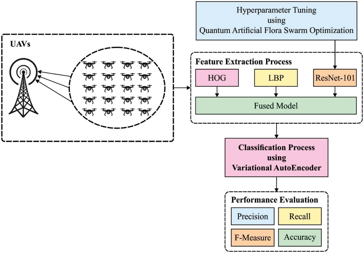
Figure 1: Working process of MMF-EDC model

3.1 Fusion of Feature Extraction

Initially, the remote sensing input images are fed into the feature extraction module to generate a useful set of feature vectors. In this study, HOG, LBP, and ResNet models are applied as feature extractors. Then, the resultant features are fused by the use of entropy technique.

3.1.1 HOG Features

A key factor in HOG feature can keep the local occurrence of objects and describe the invariance of object conversion and illumination state as edge and data about gradient is calculated with many coordinate HOG feature vectors. Initial, a gradient operator N was employed for determining the gradient measure [20]. The gradient point of mammogram image is introduced as G and image frame is displayed in I. A general equation utilized in estimating gradient point is demonstrated by Eq. (1):

Gx=N∗I(x,y)and  Gx=NT∗I(x,y)(1)

The image detection window endures classification as different spatial regions which are so called cells. Thus, the magnitude gradient of pixel is designed with edge orientation. Consequently, the magnitude of gradients (x, y) is provided by Eq. (2).

Gx(x,y)=Gx(x,y)2+Gy(x,y)2  (2)

The edge orientation of point (x, y) is implied by Eq. (3):

θ(x,y)=tan−1Gy(x,y)Gx(x,y)(3)

where Gx denotes horizontal direction of gradient and Gy represents vertical direction of gradient. In event of improved noise and illumination, a normalization function is processed when finishing the histogram measure. The establishment of normalization is utilized conversely and local histogram is authenticated. In many coordinates of HOG, four different methods of normalization are employed such as L1-norm, L2-norm, L1-Sqrt, and L2-Hys. In relation to normalization, L2-norm is given an optimum task in cancer forecast. The segment of normalization in HOG is given by Eq. (4).

L2−norm:    f=h||h||22+e2(4)

where e denotes smaller positive value utilized in regularization, f denotes feature vector, h indicates non-normalized vector, and ||h||22 so-called 2-norm of HOG normalization.

3.1.2 LBP Features

LBP module is employed in image processing applications [21]. In LBP, the histogram is integrated into a separate vector and consider a pattern vector. In other applications, the combination between LBP texture feature and Self-Organizing Maps is utilized to identify the module performance. It is determined as the operator to texture definition that is based on the sign of differences between central and neighbor pixels. The major technique of LBP operator employs the measure of centre pixel as threshold for 3×3 neighbour pixels. The threshold process can improve binary pattern which displays texture features. The operation of LBP is represented by

LBP(uc,  vc)=∑n=07⁡2ng(In−I(uc,  vc))(5)

LBP(uc,  vc) determines LBP value at intermediate pixel (uc,  vc). In and I(uc,  vc) represents values of nearby and central pixels respectively. Index n denotes index of neighbour pixel. The function g(u) will be zero if u<0 and g(u)=1 when u≥0. The contiguous pixel will be zero if the values are smaller than threshold. On the other hand, it would be one, if the neighbour pixel is greater when compared to threshold. The LBP value is defined by scalar multiplication between the binary and weight matrices. Later, the association of multiplication outcome was employed for denoting LBP value.

3.1.3 Deep Features Using ResNet Model

ResNet is one of the popular DL models which is designed with the application of residual elements. All remaining units can be given by:

yl=h(xl)+RF_(xl,  wl)(6)

xl+1=f(yl)(7)

where RF_ represents the residual function, f denotes ReLU function, wl indicates weight matrix, and xl and yl represents inputs and outputs of l-th layer [22]. The efficiency of h is assumed to be an identity mapping as follows:

h(xl)=xl(8)

The residual function RF_ is given by:

RF_(xl,  wl)=wl.  σ(B(wl′)⋅σ(B(xl))(9)

where B(xl) denotes batch normalization, ``⋅'' indicates convolution and σ(x)=  max  (x,  0). The fundamental proposal of residual learning is emerging several branches of paths which results in gradient propagation. For CNN, it was employed that equivalent path has occurred in inception methods. The residual network can distribute smaller identities together with high networks such as shortcut links and remaining blocks. However, the last outcome of all paths existing with the highway scheme can be handled by gating operation which is learned at the time of training phase. In this study, ResNet-101 model is employed.

3.1.4 Parameter Optimization Using QAFO Algorithm

During the parameter optimization process, the hyperparameters in the ResNet model such as learning rate, number of hidden layers, and their number of neurons are optimally decided by the QAFO algorithm. The AFO [23] is mainly stimulated by the migration and reproductive behavior of flora. In the AFO, the raw plants are produced primarily and they disperse seeds called offspring plants to a particular distance. It can be mathematically defined as follows. At the beginning stage, the initial population is arbitrarily created with N actual plants.

Xi,j=r×D×2−D(10)

where the input plants’ position is denoted by Xi,j, i and j are dimensions and plant count, and r denotes an arbitrary number in the range (0,1). Afterward, the propagation distance Dj is determined for all the plants. The dispersion distance of the plant is based on the dispersion distance of the preceding two rounds.

Dj=D1j×r×c1+D2j×r×c2(11)

where D2j and D1j   indicates the spreading distances parent and grandparent plants, c1 and c2 are the learning coefficients. The dispersion distance of the new grandparent plant can be defined as follows.

D1j′=D2j(12)

Besides, the new parent propagation distance can be equated using Eq. (13):

D2j′=∑i=1N⁡(Xij−Xij′)2N(13)

The position of the offspring plant over the input plant is determined using Eq. (14):

Xi,j×m′=Rij×m+Xi,j(14)

where Xij′ is the position of the offspring plant, m indicates offspring count for every plant, and Ri,j×m is a usually distributed random number with mean 0 and variance Dj. Few of the produced offsprings survive and few of them do not survive, which can be computed using the survival probability depending upon proportionate-based selection.

p=  |F(Xij×m′)F  max  |×Q(j×˙m−1)(15)

where the selective probability is denoted by Q(j×m−1) and its value is between 0 and 1, F  max   represents the upper fitness of every offspring, and the fitness of every offspring plant is F(Xi,j×m′).

To improve the performance of the AFO algorithm, quantum computing (QC) concept is integrated into it and derived from the QAFO algorithm. Quantum computing is a current technology that is interested in quantum computers by phenomena of quantum mechanics like quantum gate, state superposition, and entanglement [24]. The basic data unit in quantum computing is the Q bit. A Q bit might be in the state |0⟩, in the state |1⟩or from superposition of the states |0⟩and|1>   concurrently. Based on Dirac notation, the Q bit is denoted by the integration of the states |0>and|1> is given by:

|Q⟩=α|0⟩+β|1⟩  such  that|α|2+|β|2=1(16)

where α and β represents complex number. |α|2 (resp. |β|2) indicates likelihood for finding Q bit in state zero (represented in state 1). A quantum register of size n is later established from a set of nQ bits. It denotes a superposition of nQ bits, especially, it has up to 2n probable values consecutively. A quantum register is denoted as:

Ψ=∑x=02n−1⁡CX|X⟩(17)

The amplitudes CX fulfill the succeeding equation:

∑x=02n−1⁡|CX|2=1(18)

The state of a Q bit is altered by a quantum gate (Q-gate). A Q gate represents reversible gate and unitary operator U act on the Q bit bases state fulfilling U+U=UU+, whereas U+ indicates Hermitian adjoint of U. It consists of various Q gates, like Hadamard gate, NOT gate, rotation gate, controlled NOT gate, and so on.

3.1.5 Fusion Model

In this study, data fusion is employed to fuse the features from three models. The fusion feature is a significant process that integrated several feature vectors. The proposed method is depending upon fusion feature using entropy.

The 3 vectors are given by:

fHOG1  ×  n  =  {HOG1×1,  HOG1×2,  HOG1×3,…,HOG1×n}(19)

fLBP1  ×p={LBP1×1,LBP1×2,LBP1×3,…,LBP1×n}(20)

fRes191×m={RES1911×1,  RES1911×2,  RES1911×3,…RES1911×n}(21)

Furthermore, feature extraction is combined in an individual vector.

Fused  (features  vector)1×q=  ∑i=13⁡{fHOG1  ×  n,  fVRES191×m,  fLBP1  ×p}(22)

where f denotes fused vector (1  ×1186). The entropy is employed on the feature vectors for selecting optimum features depending upon score [25]. The FS task is scientifically described by Eqs. (19)–(22).

BHe=−NHeb∑i=1n⁡p(fi)(23)

Fselect=BHe(max(fi,  1186))(24)

In Eqs. (23) and (24), p denotes feature likelihood and He indicates entropy. The lastly selected feature is provided for the VAE classification model to distinguish the remote sensing images.

3.2 VAE Based Scene Classification

During the classification process, the fused features are fed into the VAE model to allot the proper class labels. Autoencoder (AE) is one of the initial generative modules trained for recreating/reproducing the input vector x. The AE is consisting of 2 major frameworks: encoder and decoder, that is multilayered (NN) parameterized using φ and θ, correspondingly. The initial portion encodes the input data x to a latent depiction z using encoder function =fφ(x), where the next NN decodes this latent depiction to X =h(z) that is a reconstruction/approximation of the novel data.

The variant form of the AE turns into a common generative module with the combination of Bayesian inference and effectiveness of the NN is to attain a non-linear low dimension latent space [26]. The Bayesian inference is attained with other layers utilized to sample the latent vector z with previously stated distribution p(z), typically consider to be a regular Gaussian N(0,I), whereas I denote identity matrix. Every element zi of the latent layer is attained by:

zi=μi+σi.e(25)

whereas μi and σi represents ith component of the standard deviation and mean vectors, e indicates arbitrary parameter succeeding a regular Normal distribution (  e∼N(0,1)). Contrasting the AE, that produces latent vector z, the VAE produces vector of means μj and standard deviations σi. This permits to have additional continuousness in the latent space compared to original AE. The VAE loss function is denoted in Eq. (26) contain 2 expressions. The initial term Lrec represents recreation loss function (Eq. (27)), that enables minimizing the variance among input and output samples. Fig. 3 showcases the architecture of VAE.

Both negative expected   log   probability (for example the cross entropy function) and mean squared error (MSE) are utilized. While the sigmoid function is utilized in the output layer, the derivative of MSE and cross entropy could contain equivalent formations. The next term Lkl (Eq. (28)) equivalent to the KullbackLiebler (Dkl) divergence loss term which forces the generation of latent vector with the stated Normal distribution. The Dkl divergence is a theoretic measure of proximity among 2 densities q(x) and p(x). It is asymmetric (Dkl(q||p)≠Dkl(p||q)) and non-negative. It is reduced when q(x)=p(x). Therefore, the Dkl divergence terms measure the conditional distribution density qφ(z|x) of encoded latent vector is from the desired Normal distribution p(z). The value of Dkl is 0 if 2 likelihood distributions are similar, that forces the encoder of VAE qφ(z|x) for learning the latent parameter which follows a multivariate normal distribution on a k dimension latent space.

L=Lrec+Lkl(26)

Lrec=−Eqφ(z|x)[logpθ(x|z)](27)

Lkl=Dkl(qφ(z|x)||p(z))(28)

4  Performance Validation

This section validates the performance of the presented model on two datasets namely UCM and WHU-RS dataset [27]. The proposed model is simulated using MATLAB. The details compared to the dataset are provided in Tab. 1. The first UCM dataset holds a set of 100 images with 21 classes and the WHU-RS dataset holds a total of 950 images with 19 classes.

A detailed comparative results analysis of the MMF-EDC model with other models on the applied UCM dataset is given in Tab. 2 and Fig. 2. The experimental results showcased that the proposed MMF-EDC model accomplished maximum classification outcome under varying amounts of training data.

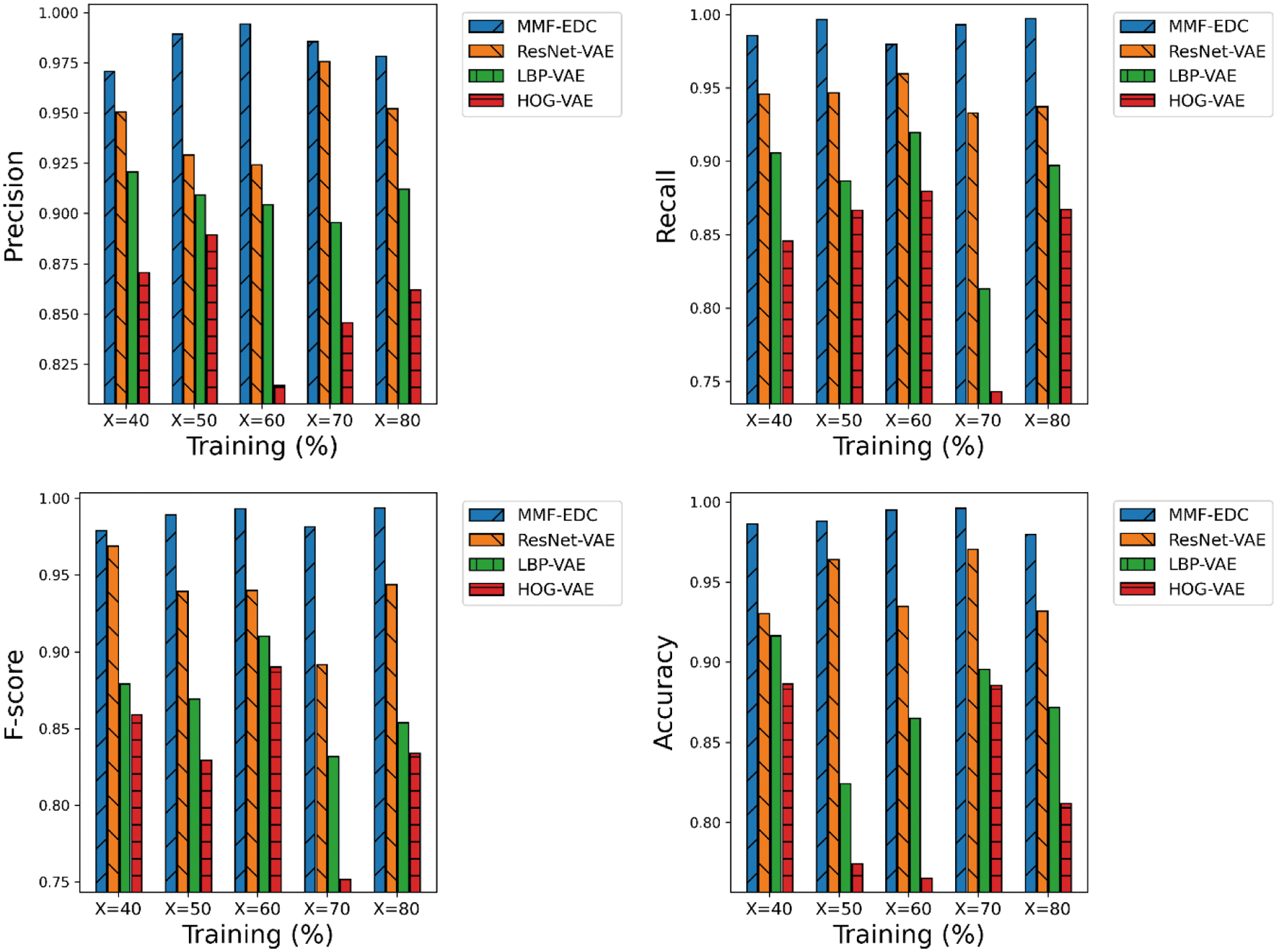
Figure 2: Comparative analysis of MMF-EDC model on UCM dataset

Simultaneously, the HOG-VAE model has attained minimum classifier results over the other methods. Though the ResNet-VAE and LBP-VAE models have demonstrated moderate performance, they failed to outperform the MMF-EDC model. For instance, the MMF-EDC model has offered a higher average precision of 0.9836 whereas the ResNet-VAE, LBP-VAE, and HOG-VAE models have exhibited lower average precision of 0.9506, 0.9206, and 0.8706 respectively. Additionally, the MMF-EDC model has offered a higher average recall of 0.9903 whereas the ResNet-VAE, LBP-VAE, and HOG-VAE models have exhibited lower average recall of 0.9443, 0.8843, and 0.8403 respectively. Simultaneously, the MMF-EDC model has offered a higher average F-score of 0.9836 whereas the ResNet-VAE, LBP-VAE, and HOG-VAE models have exhibited lower average F-score of 0.9873, 0.9366, and 0.8686 respectively. At last, the MMF-EDC technique has offered a higher average accuracy of 0.9890 whereas the ResNet-VAE, LBP-VAE, and HOG-VAE models have exhibited lower average accuracy of 0.9463, 0.8745, and 0.8245 respectively.

A detailed comparative results analysis of the MMF-EDC model with other models on the applied WHU-RS dataset is given in Tab. 3 and Fig. 3. The experimental results showcased that the proposed MMF-EDC model accomplished maximum classification outcome under varying amounts of training data. Likewise, the HOG-VAE algorithm has attained minimum classifier results over the other methods. Though the ResNet-VAE and LBP-VAE models have demonstrated moderate performance, they failed to outperform the MMF-EDC model. For instance, the MMF-EDC model has offered a higher average precision of 0.9961 whereas the ResNet-VAE, LBP-VAE, and HOG-VAE models have exhibited lower average precision of 0.9195, 0.8455, and 0.8255 respectively. Additionally, the MMF-EDC model has offered a higher average recall of 0.9835 whereas the ResNet-VAE, LBP-VAE, and HOG-VAE models have exhibited lower average recall of 0.9505, 0.8925, and 0.8545 respectively. Simultaneously, the MMF-EDC model has offered a higher average F-score of 0.9806 whereas the ResNet-VAE, LBP-VAE, and HOG-VAE models have exhibited lower average F-score of 0.9206, 0.8586, and 0.8466 respectively.

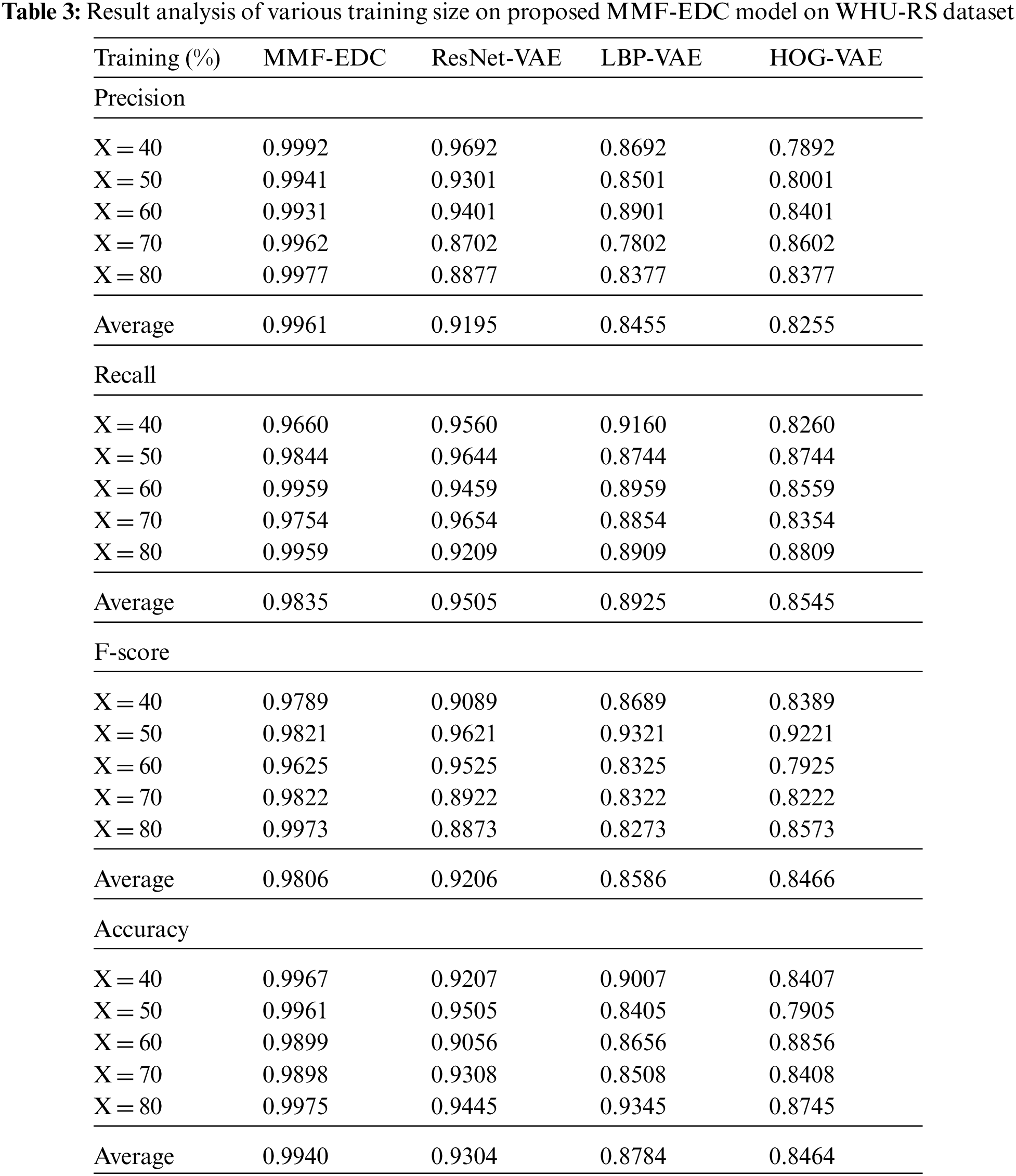
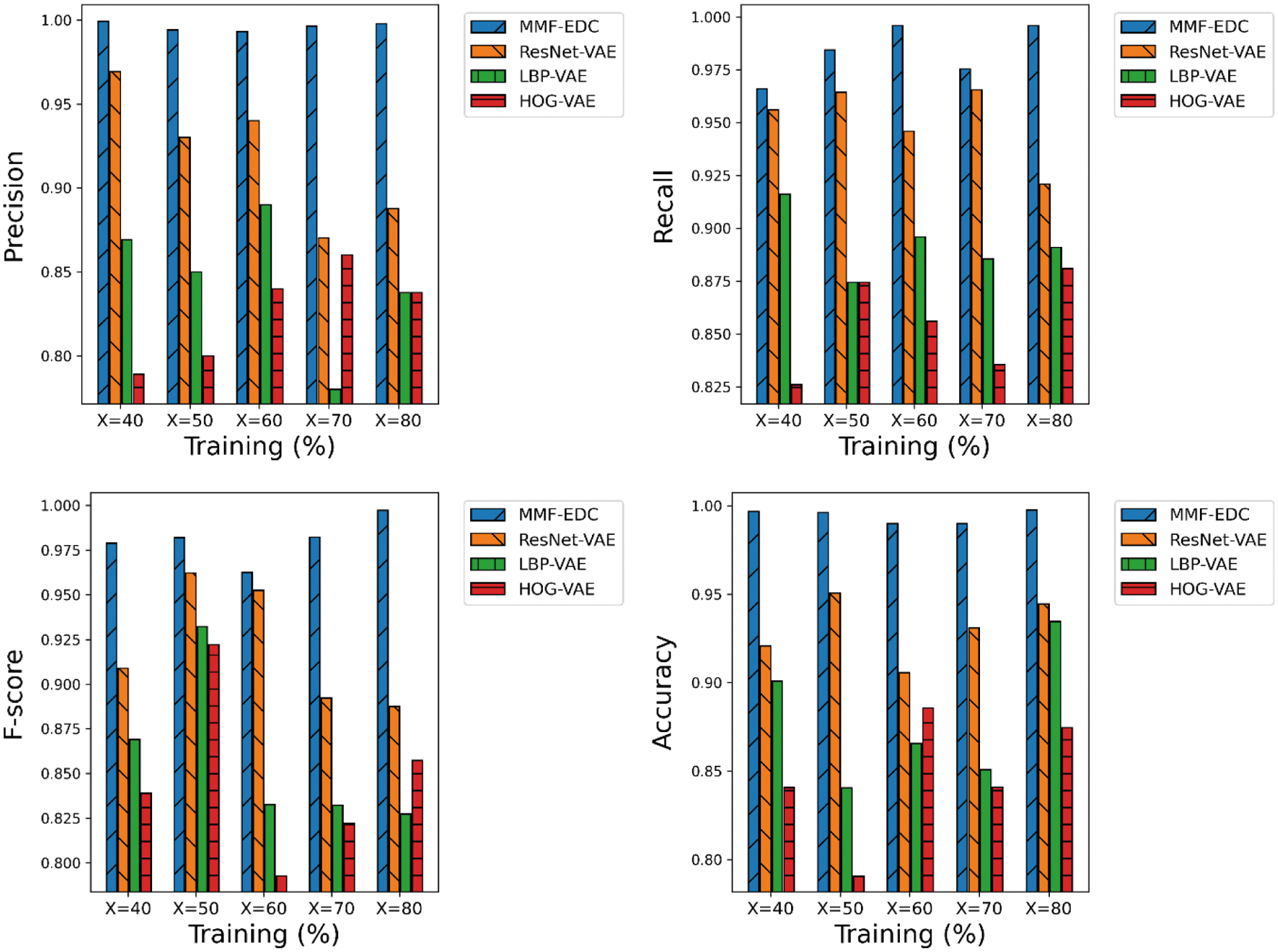
Figure 3: Comparative analysis of MMF-EDC model on WHU-RS dataset

At last, the MMF-EDC technique has offered a higher average accuracy of 0.9940 whereas the ResNet-VAE, LBP-VAE, and HOG-VAE models have exhibited lower average accuracy of 0.9304, 0.8784, and 0.8464 respectively. A brief comparative results analysis of the MMF-EDC model with other existing methods interms of accuracy is provided in Tab. 4 and Fig. 4. From the obtained results, it is evident that the PlacesNet model has appeared as poor performance with the accuracy of 0.91 and 0.92 on test UCM and WHU-RS datasets. Then, the VGG-VD19 model has obtained slightly enhanced outcome with the accuracy of 0.93 and 0.94 on test UCM and WHU-RS dataset.

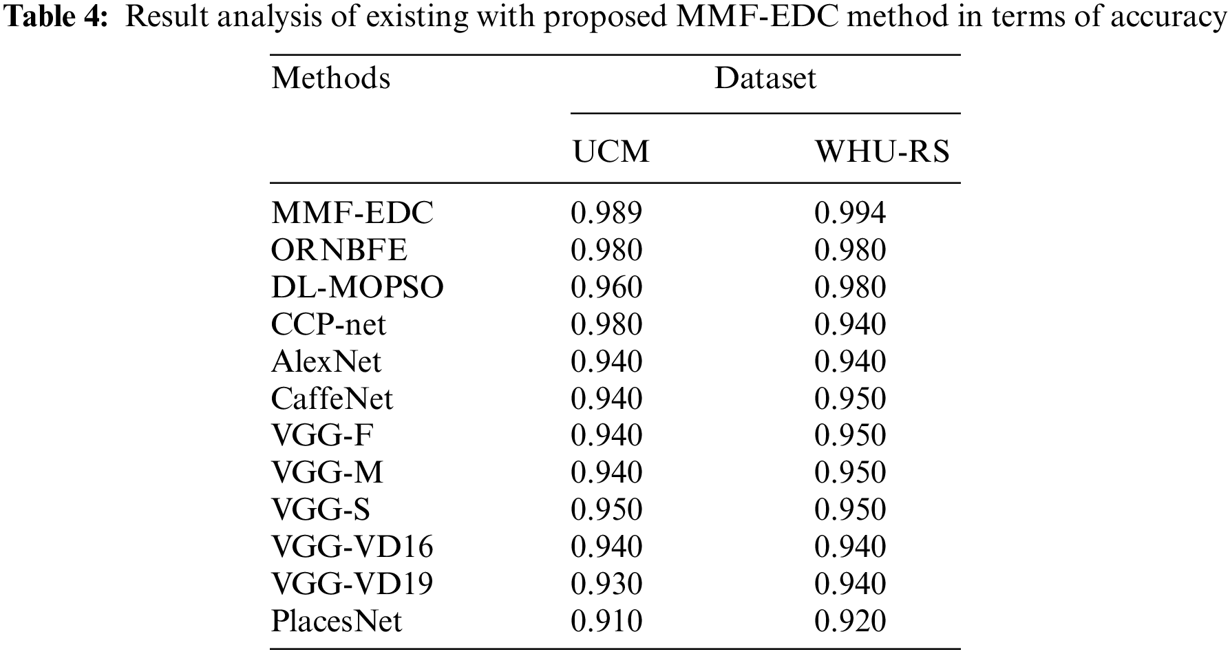
Figure 4: Result analysis of MMF-EDC model interms of accuracy

Afterward, the AlexNet model has attained further enhanced results with the accuracy of 0.94 and 0.94 on test UCM and WHU-RS datasets. Followed by, the CaffeNet, VGG-F, VGG-M, VGG-VD-16, and VGG-S models have showcased moderately closer accuracy values on test UCM and WHU-RS dataset. Simultaneously, the deep learning with multi-objective particle swarm optimization (DL-MOPSO) model has exhibited slightly reasonable outcome with the accuracy of 0.96 and 0.98 on test UCM and WHU-RS datasets. Concurrently, the ORNBFE model has resulted in a nearly acceptable outcome with the accuracy of 0.98 and 0.98 on test UCM and WHU-RS datasets. Eventually, the CCP-Net model has gained competitive performance with the accuracy of 0.98 and 0.94 on test UCM and WHU-RS datasets. However, the proposed MMF-EDC model has accomplished superior performance with the accuracy of 0.989 and 0.994 on test UCM and WHU-RS datasets.

A brief comparative outcomes analysis of the MMF-EDC model with other existing models with respect to computation time (CT) is given in Tab. 5 and Fig. 5. From the attained outcomes, it can be clear that the VGGNet technique is revealed as the worst performance with CT of 500 s and 560 s on test UCM and WHU-RS dataset. Then, the VGG-VD16 model has obtained slightly enhanced outcome with the CT of 415 s and 480 s on test UCM and WHU-RS dataset. Later, the VGG-S model has attained further enhanced results with the CT of 135 s and 156 s on test UCM and WHU-RS datasets.

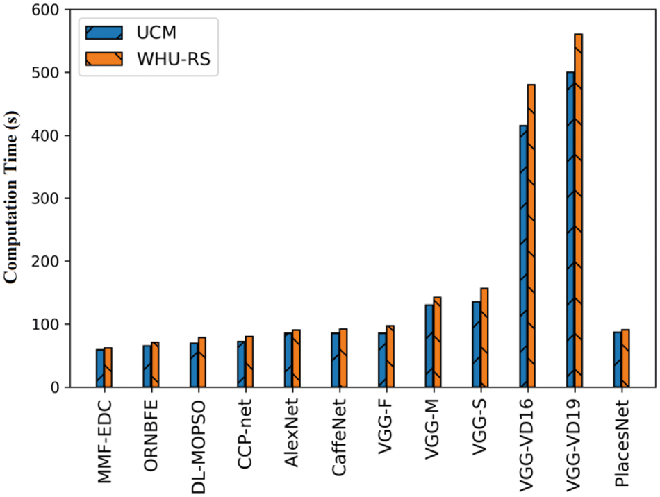
Figure 5: Computation time analysis of MMF-EDC model

In the meantime, the VGG-M approach has resulted in a certainly increased result with CT of 130 s and 142 s on test UCM and WHU-RS dataset. Followed by, the PlacesNet, AlexNet, CaffeNet, and VGG-F techniques have depicted moderately closer CT values on test UCM and WHU-RS dataset. Concurrently, the CCP-net model has exhibited slightly reasonable results with the CT of 72 s and 80 s on test UCM and WHU-RS datasets. Concurrently, the DL-MOPSO model has resulted in a nearly acceptable result with the CT of 69 s and 78 s on test UCM and WHU-RS datasets. Finally, the ORNBFE model has gained competitive performance with the CT of 65 s and 71 s on test UCM and WHU-RS datasets. However, the proposed MMF-EDC model has accomplished higher performance with the CT of 59 s and 62 s on test UCM and WHU-RS datasets.

From the above mentioned experimental results analysis, it is obvious that the proposed MMF-EDC model is found to be an appropriate scene classification tool for RS data. The proposed MMF-EDC model not only achieves higher classification accuracy, it also achieves minimum computation complexity.

5  Conclusion

This paper has presented an effective MMF-EDC model for pattern identification in the earth data and classifies them into appropriate class labels. The proposed MMF-EDC model aims to identify and classify the scenes that exist in the remote sensing data, which is helpful for several real time applications. The MMF-EDC technique involves two major phases namely feature fusion and classification. Primarily, the features in the input remote sensing images are extracted using HOG, LBP, and QAFO-ResNet models, which are then are fused by the use of entropy technique. The application of QAFO algorithm helps to increase the classification performance of the presented method by optimally tuning the hyperparameters of the ResNet model. Besides, the VAE model is applied to categorize the scenes based on the fused feature vectors. The experimental assessment of the MMF-EDC model is carried out on benchmark UCM and WHU-RS datasets. The experimental values denoted that the MMF-EDC method exhibit promising classification performance on all the applied images with maximum accuracy of 0.989 and 0.994 on the test UCM and WHU-RS dataset respectively. In future, the performance of the MMF-EDC technique is enhanced with utilize of advanced DL architectures for image classification process.

Funding Statement: The authors would like to thank the Taif University for funding this work through Taif University Research Supporting, Project Number. (TURSP-2020/277), Taif University, Taif, Saudi Arabia.

Conflicts of Interest: The authors declare that they have no conflicts of interest to report regarding the present study.

References

 1.  J. Song, S. Gao, Y. Zhu and C. Ma, “A survey of remote sensing image classification based on CNNs,” Big Earth Data, vol. 3, no. 3, pp. 232–254, 2019. [Google Scholar]

 2.  S. K. Lakshmanaprabu, K. Shankar, S. S. Rani, E. Abdulhay, N. Arunkumar et al., “An effect of big data technology with ant colony optimization based routing in vehicular ad hoc networks: Towards smart cities,” Journal of Cleaner Production, vol. 217, pp. 584–593, 2019. [Google Scholar]

 3.  J. Uthayakumar, T. Vengattaraman and J. Amudhavel, “Data compression algorithm to maximize network lifetime in wireless sensor networks,” Journal of Advanced Research in Dynamical and Control, vol. 9, pp. 2156–2167, 2017. [Google Scholar]

 4.  X. Xu, Y. Chen, J. Zhang, Y. Chen, P. Anandhan et al., “A novel approach for scene classification from remote sensing images using deep learning methods,” European Journal of Remote Sensing, vol. 54, no. sup2, pp. 383–395, 2021. [Google Scholar]

 5.  S. C. Hung, H. C. Wu and M. H. Tseng, “Remote sensing scene classification and explanation using RSSCNet and LIME,” Applied Sciences, vol. 10, no. 18, pp. 6151, 2020. [Google Scholar]

 6.  L. N. Smith, “Cyclical learning rates for training neural networks,” in 2017 IEEE Winter Conf. on Applications of Computer Vision (WACV), Santa Rosa, CA, USA, pp. 464–472, 2017. [Google Scholar]

 7.  L. N. Smith and N. Topin, “Super-convergence: Very fast training of neural networks using large learning rates,” in Artificial Intelligence and Machine Learning for Multi-Domain Operations Applications, Baltimore, United States, SPIE Digital Library, 2019. [Google Scholar]

 8.  G. Leclerc and A. Madry, “The two regimes of deep network training,” Machine Learning, pp. 1–14, 2020. [Google Scholar]

 9.  Z. Li, H. Shen, Y. Wei, Q. Cheng and Q. Yuan, “Cloud detection by fusing multi-scale convolutional features,” in Proc. of the ISPRS Annals of the Photogrammetry, Remote Sensing and Spatial Information Science, Beijing, China, pp. 7–10, 2018. [Google Scholar]

10. C. Zhang, I. Sargent, X. Pan, H. Li, A. Gardiner et al., “Joint deep learning for land cover and land use classification,” Remote Sensing of Environment, vol. 221, pp. 173–187, 2019. [Google Scholar]

11. A. Prathik, J. Anuradha and K. Uma, “A novel algorithm for soil image segmentation using colour and region based system,” International Journal of Innovative Technology and Exploring Engineering, vol. 8, no. 10, pp. 3544–3550, 2019. [Google Scholar]

12. M. Kampffmeyer, A. B. Salberg and R. Jenssen, “Urban land cover classification with missing data modalities using deep convolutional neural networks,” IEEE Journal of Selected Topics in Applied Earth Observations and Remote Sensing, vol. 11, no. 6, pp. 1758–1768, 2018. [Google Scholar]

13. R. Interdonato, D. Ienco, R. Gaetano and K. Ose, “DuPLO: A DUal view point deep learning architecture for time series classification,” ISPRS Journal of Photogrammetry and Remote Sensing, vol. 149, pp. 91–104, 2019. [Google Scholar]

14. N. S. Murugan and G. U. Devi, “Feature extraction using LR-PCA hybridization on twitter data and classification accuracy using machine learning algorithms,” Cluster Computing, vol. 22, no. S6, pp. 13965–13974, 2019. [Google Scholar]

15. H. Wang, X. Zhao, X. Zhang, D. Wu and X. Du, “Long time series land cover classification in China from 1982 to 2015 based on Bi-LSTM deep learning,” Remote Sensing, vol. 11, no. 14, pp. 1639, 2019. [Google Scholar]

16. C. Shi, Z. Lv, X. Yang, P. Xu and I. Bibi, “Hierarchical multi-view semi-supervised learning for very high-resolution remote sensing image classification,” Remote Sensing, vol. 12, no. 6, pp. 1012, 2020. [Google Scholar]

17. Y. Dong, T. Liang, Y. Zhang and B. Du, “Spectral–spatial weighted kernel manifold embedded distribution alignment for remote sensing image classification,” IEEE Transactions on Cybernetics, vol. 51, no. 6, pp. 3185–3197, 2021. [Google Scholar]

18. M. P. Uddin, M. A. Mamun and M. A. Hossain, “PCA-based feature reduction for hyperspectral remote sensing image classification,” IETE Technical Review, vol. 38, no. 4, pp. 377–396, 2021. [Google Scholar]

19. C. Zhang, Y. Chen, X. Yang, S. Gao, F. Li et al., “Improved remote sensing image classification based on multi-scale feature fusion,” Remote Sensing, vol. 12, no. 2, pp. 213, 2020. [Google Scholar]

20. R. Suresh, A. N. Rao and B. E. Reddy, “Detection and classification of normal and abnormal patterns in mammograms using deep neural network,” Concurrency and Computation: Practice and Experience, vol. 31, no. 14, pp. 1–12, 2019. [Google Scholar]

21. E. Prakasa, “Texture feature extraction by using local binary pattern,” INKOM, vol. 9, no. 2, pp. 45, 2016. [Google Scholar]

22. S. Wan, Y. Liang and Y. Zhang, “Deep convolutional neural networks for diabetic retinopathy detection by image classification,” Computers & Electrical Engineering, vol. 72, pp. 274–282, 2018. [Google Scholar]

23. T. Bezdan, E. Tuba, I. Strumberger, N. Bacanin and M. Tuba, “Automatically designing convolutional neural network architecture with artificial flora algorithm,” in ICT Systems and Sustainability, Singapore: Springer, pp. 371–378, 2020. [Google Scholar]

24. D. Zouache, F. Nouioua and A. Moussaoui, “Quantum-inspired firefly algorithm with particle swarm optimization for discrete optimization problems,” Soft Computing, vol. 20, no. 7, pp. 2781–2799, 2016. [Google Scholar]

25. T. Saba, A. S. Mohamed, M. E. Affendi, J. Amin and M. Sharif, “Brain tumor detection using fusion of hand crafted and deep learning features,” Cognitive Systems Research, vol. 59, pp. 221–230, 2020. [Google Scholar]

26. R. Zemouri, “Semi-supervised adversarial variational autoencoder,” Machine Learning and Knowledge Extraction, vol. 2, no. 3, pp. 361–378, 2020. [Google Scholar]

27. Y. Yang and S. Newsam, “Bag-of-visual-words and spatial extensions for land-use classification,” in Proc. of the 18th SIGSPATIAL Int. Conf. on Advances in Geographic Information Systems-GIS ‘10, San Jose, California, pp. 270, 2010. [Google Scholar]

This work is licensed under a Creative Commons Attribution 4.0 International License, which permits unrestricted use, distribution, and reproduction in any medium, provided the original work is properly cited.