DOI:10.32604/cmc.2022.022593
| Computers, Materials & Continua DOI:10.32604/cmc.2022.022593 | |
| Article |
A Deep Learning Hierarchical Ensemble for Remote Sensing Image Classification
1Department of Computer Engineering, Anyang University, Anyang-si, 14028, Korea
2Department of ICT Convergence Engineering, Anyang University, Anyang-si, 14028, Korea
*Corresponding Author: Jeong-Joon Kim. Email: jjkim@anyang.ac.kr
Received: 12 August 2021; Accepted: 13 September 2021
Abstract: Artificial intelligence, which has recently emerged with the rapid development of information technology, is drawing attention as a tool for solving various problems demanded by society and industry. In particular, convolutional neural networks (CNNs), a type of deep learning technology, are highlighted in computer vision fields, such as image classification and recognition and object tracking. Training these CNN models requires a large amount of data, and a lack of data can lead to performance degradation problems due to overfitting. As CNN architecture development and optimization studies become active, ensemble techniques have emerged to perform image classification by combining features extracted from multiple CNN models. In this study, data augmentation and contour image extraction were performed to overcome the data shortage problem. In addition, we propose a hierarchical ensemble technique to achieve high image classification accuracy, even if trained from a small amount of data. First, we trained the UC-Merced land use dataset and the contour images for each image on pretrained VGGNet, GoogLeNet, ResNet, DenseNet, and EfficientNet. We then apply a hierarchical ensemble technique to the number of cases in which each model can be deployed. These experiments were performed in cases where the proportion of training datasets was 30%, 50%, and 70%, resulting in a performance improvement of up to 4.68% compared to the average accuracy of the entire model.
Keywords: Image classification; deep learning; CNNs; hierarchical ensemble; UC-Merced land use dataset; contour image
Recently, demand and use cases of big data have been increasing in various industries, and owing to the rapid development of artificial intelligence, it has drawn attention as a tool to solve various problems demanded by society and industry. In particular, research on land-use classification in remote sensing fields is actively underway, and related high-resolution spatial image data can be obtained. In addition, innovative advances in computer vision field technology create a variety of opportunities to improve remote sensing image recognition and classification performance, facilitating the development of new approaches. The classification of land use in remote sensing images is critical for analyzing, managing, and monitoring the land use areas of people. In addition, deep learning-based classification techniques are needed to analyze environmental pollution, natural disasters, and land changes caused by human development in consideration of the complex geographical characteristics and diversity of images according to the weather.
Traditional image recognition techniques have used methods such as SIFT [1], HOG [2], and BoVW [3] to extract numerous features from images and search for the location of objects using extracted features. However, there is a disadvantage in that the classification accuracy for new images is low because of their sensitivity to shape transformation or brightness conditions.
CNNs, which have recently been studied in various ways, were first introduced in [4] to process images more effectively by applying filtering techniques to artificial neural networks, and later proposed CNNs, which are currently being used in the deep learning field in [5]. AlexNet [6], which won the ImageNet Large Scale Visual Registration (ILSVRC) competition held in 2012, is still widely used in image recognition and classification, object detection, and tracking and shows excellent performance [7]. VGGNet [8], GoogLeNet [9], ResNet [10], DenseNet [11], and EfficientNet [12] recently achieved superior performance in image recognition and classification.
Additionally, in recent years, when image classification is performed to complement the performance of a single CNN architecture, ensemble techniques have emerged that harmoniously utilize predictive results from multiple well-designed deep learning architectures. By training several models, a combination of the predicted results of these models were used to obtain more accurate predictions. Recently, research has been actively conducted on the application of deep learning ensemble techniques in various fields [13–17].
In this study, we used transfer learning strategies to overcome overfitting and improve the convergence rate of the models. Using a pretrained CNN architecture is the preferred method in several existing studies [18–21]. The UC-Merced land use dataset [22] was used to evaluate the experimental performance, and six scenarios were set according to whether the contour image was trained and the ratio of the training data, and then individually trained on five pretrained CNN architectures with excellent performance. We then performed hierarchical ensembles on the number of cases in which the five learning models can be deployed. The method proposed in this study was named hierarchical ensembles because the output values of the previous layer were used as inputs for the next layer. The three contributions of this study are summarized as follows.
• We demonstrate that learning contour images to classify remote sensing images using a CNN architecture is an important factor in performance improvement.
• We propose a hierarchical ensemble technique to complement the poor performance of a single model and achieve higher image classification accuracy.
• We achieve excellent image classification performance even if we use CNN models with a small amount of training data through the learning of contour images and hierarchical ensembles.
The remainder of this paper is organized as follows. Section 2 introduces the related work. Section 3 describes the dataset used in this study and the experimental method in detail. Section 4 presents the experimental results and analyses. Section 5 concludes this paper and suggests directions for future research.
2 Convolutional Neural Networks
As shown in Fig. 1, CNN uses convolutional layers to extract feature maps for input images and pooling layers to convert the local parts of each feature map into one representative scalar value. In addition, the derived feature maps were utilized to configure the classification operation on the image to be performed.

Figure 1: Basic architecture of CNNs
CNNs can generally be formulated as shown in Eq. (1).
VGGNet is a model developed by the University of Oxford Visual Geometry Group that won second place in the 2014 ILSVRC competition. The VGG research team proposed six models to compare the performance of neural networks according to depth. Among them, VGG16 with 13 conv layers, three FC layers, and VGG19 with 16 conv layers and three FC layers were used. In this work, we used VGG19, and the architectures of VGG16 and VGG19 are shown in Figs. 2 and 3.

Figure 2: VGG16 architecture

Figure 3: VGG19 architecture
GoogLeNet is a neural network developed by Google that won the 2014 ILSVRC competition by beating VGGNet. Although it consists of 22 layers, deeper than VGG19, it uses

Figure 4: Inception module in GoogLeNet
ResNet is a neural network developed by Microsoft that won the ILSVRC competition in 2015. Because it is difficult to expect good performance even with the deep design of neural network models, ResNet introduced a residual block with added shortcut to the input value of neural networks to the output value. ResNet, which consists of 18, 34, 50, 101, and 152 layers, has been proposed, and ResNet-152 with 152 layers has the best performance. In this work, we use a 101-layer ResNet-101 model, which visualizes the residual block and ResNet architecture as shown in Figs. 5 and 6.

Figure 5: Residual block

Figure 6: ResNet architecture
DenseNet does not add input values to the output values, such as residual blocks. Instead, it uses dense blocks that concatenate the input and output values. Because DenseNet connects the feature maps of all layers, the information flow is improved, preventing information loss when the feature map passes through the layers of the neural network, and also reduces the vanishing gradient problem. DenseNet composed of 121, 169, 201, and 264 layers was proposed, and in this study, DenseNet-121 composed of 121 layers was used. Fig. 7 shows a visualization of the dense block.

Figure 7: Dense block
Many of the CNN architectures that have previously emerged have evolved to scale models to achieve higher accuracy within limited resources. ResNet is a representative model of depth scaling that increases the number of layers, and representative models of width scaling that increase the number of kernels include MobileNet [24] and ShuffleNet [25]. Before EfficientNet appeared, there were no guidelines for selecting an appropriate scaling technique, thus it was difficult to prove it through experiments. EfficientNet enables efficient and effective model scaling by using the compound scaling technique that scales the model by adjusting the balance between the depth, width, and resolution of the CNN. For EfficientNet, eight models were proposed according to the scaling method, in which EfficientNetB0, the baseline model of EfficientNet, is used. Fig. 8 shows a schematic for comparing each model scaling technique.
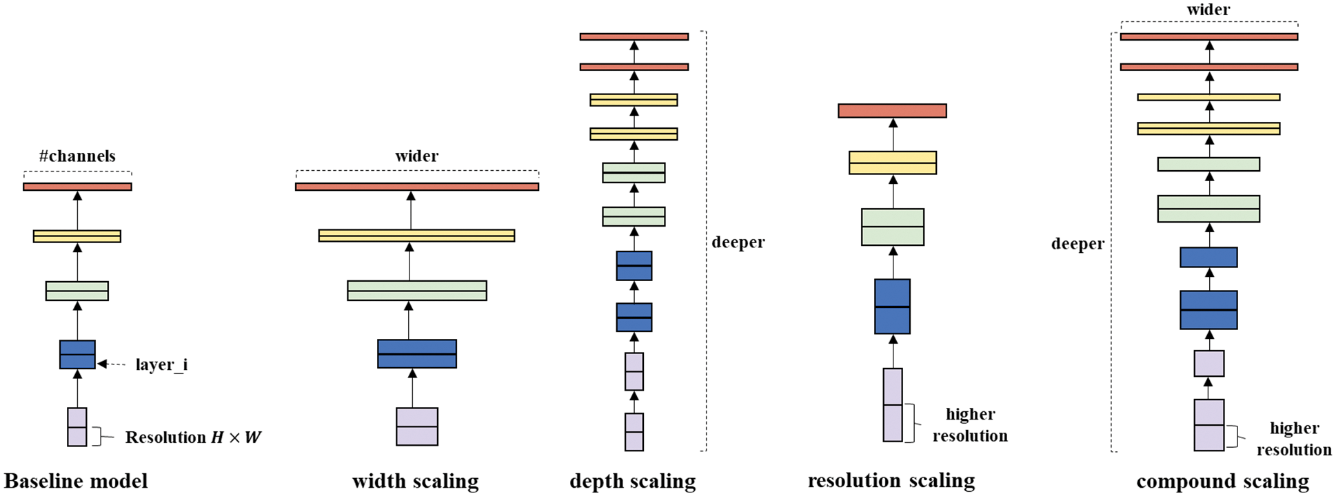
Figure 8: Model scaling methods
In this section, we first describe the dataset obtained for this experiment, and then describe the scenarios and specific steps of each experiment.
3.1 Dataset and Extraction of Contour Images
The dataset used in this study, the UC-Merced Land Use dataset, is a remote sensing image dataset for land use. It consists of 21 classes: agricultural, airplane, baseball diamond, beach, buildings, chaparral, dense residential, forest, freeway, golf course, harbor, intersection, medium residential, mobile home park, overpass, parking lot, river, runway, sparse residential, storage tank, and tennis court. It contains a total of 2100 images, including 100 images per class, and most of the images have a resolution of
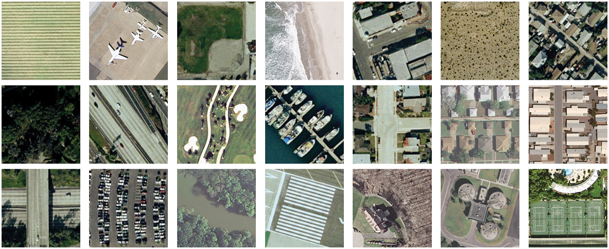
Figure 9: Sample images of UC-Merced land use dataset for 21 classes
In addition, to obtain more training datasets, each image was rotated, shifted, zoomed, and made symmetrical, and the contour image for each image was extracted to increase the size of the training dataset. Algorithms for edge extraction include Sobel [26], Prewitt [27], Roberts [28], and Canny edge detection [29]. In this study, the Canny edge detection algorithm was used. Fig. 10 shows the five steps for Canny edge detection, and the images extracted at each step. First, the result of edge detection on the input image is very sensitive to noise, so the noise is removed using a Gaussian kernel. In the second step, the intensity and direction of the edge are detected by calculating the gradient to find the point at which the pixel value changes rapidly. The image extracted at this stage contains non-edge parts. Therefore, in step 3, non-maximum suppression is performed to remove these non-edge parts. In step 4, we set the maximum and minimum thresholds to identify strong or weak edge pixels. Finally, in step 5, for pixels between the maximum and minimum thresholds, the connection structure of each pixel determines whether it is an edge.

Figure 10: Detailed steps for extraction of contours using the Canny edge detection
Fig. 11 shows a sample extracted from the original image, and this edge information is efficiently used for GIS data analysis.

Figure 11: Sample contour images from UC-Merced land use dataset for 21 classes
3.2 Experimental Scenarios and Detailed Steps
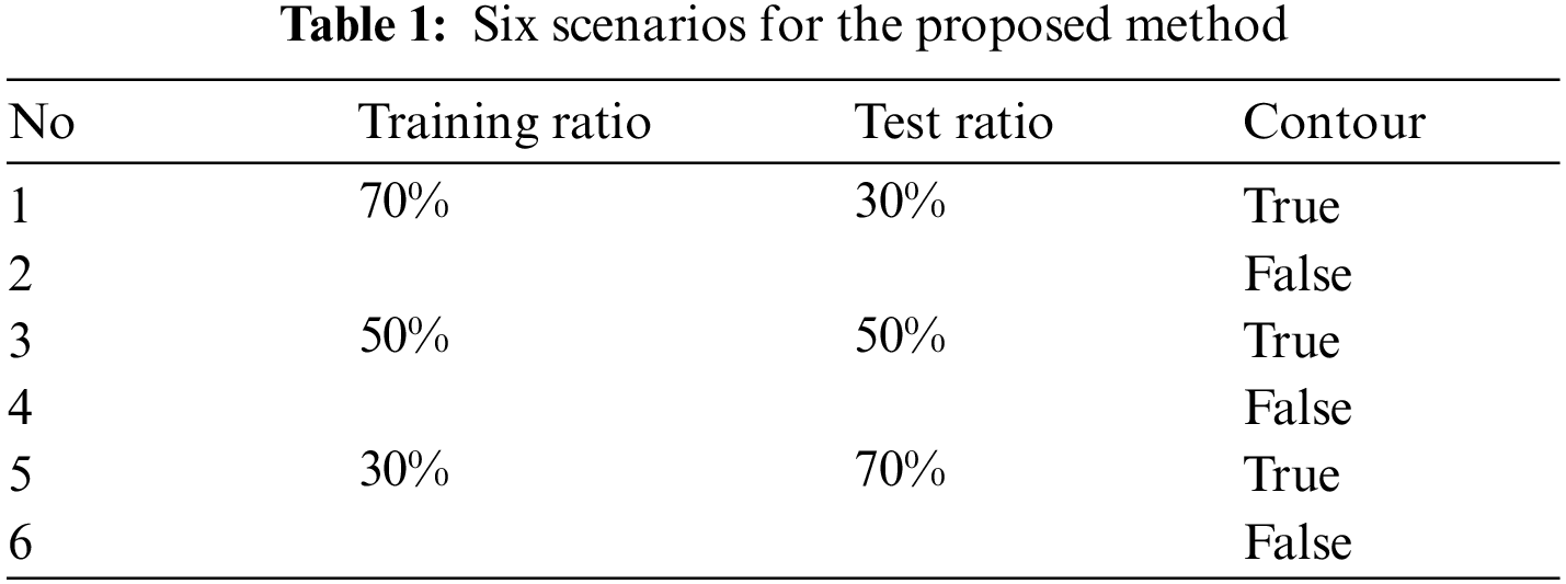
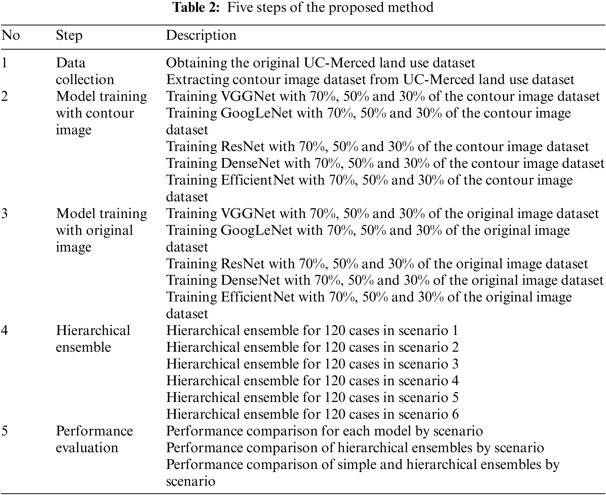
The proposed method consists of five steps: First, for the training of VGGNet, GoogLeNet, ResNet, DenseNet, and EfficientNet, six scenarios were set according to whether the contour image was trained and the ratio of the training data; detailed information of each scenario is presented in Tab. 1. When the training of each model was completed for each scenario, the hierarchical ensemble was performed by appropriately arranging the five models. The number of cases where five models could be deployed in one scenario was 120, and there were a total of 720 cases for six scenarios. The steps of the proposed study are presented in Tab. 2.
In this study, to overcome overfitting and reduce the training time, a model pretrained with the ImageNet dataset was used using transfer learning techniques, and each model was trained using a GPU. In addition, to measure the performance improvement by hierarchical ensembles according to the ratio of training data, the learning epoch of each model was set to 50, and the learning rate was fixed at 0.0001. Additionally, the Adam [30] optimizer was used to enable each model to converge quickly. Fig. 12 schematically shows the method proposed in this study. The performance process of the hierarchical ensembles is shown in Algorithm 1.
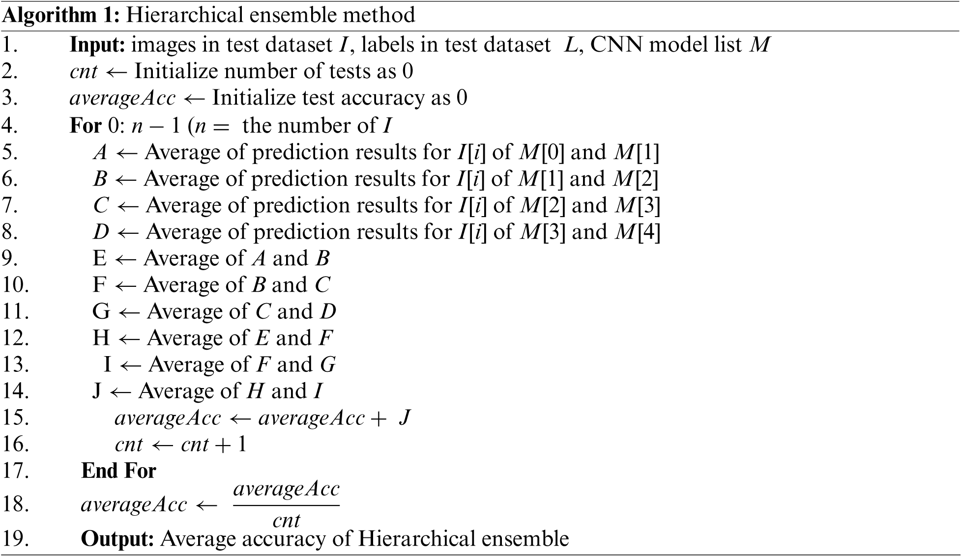

Figure 12: Diagram of the proposed method
4 Experimental Results and Discussion
The experiments performed in this study were performed on a 64-bit Windows 10 Education Operation system and were implemented using the Python programming language and the Keras library. The PC used in the experiment was equipped with an NVIDIA GeForce RTX 2070 SUPER 8 GB GPU, AMD Ryzen 7 3700X 8-Core CPU, and 32 GB RAM.
4.1 Experimental Results and Analysis for Each Model
Fig. 13 shows the classification accuracy of each model that has learned the contour image among the six scenarios proposed in this study, and Fig. 14 shows the classification accuracy of each model that does not learn the contour image. As for the classification accuracy of individual models, the model trained including the contour image had higher accuracy, and the higher the proportion of training data, the higher the accuracy. Therefore, we confirmed that learning the contour image is significant for improving the classification performance of the model. In addition, it was confirmed that the ratio of the training data affected the performance of each model. In the case of learning contour images, GoogLeNet performed best when the proportion of training data was 70%, whereas it was third when it was 30%. In the case of ResNet, when the proportion of training data was 70%, it was the third best, whereas when it was 30%, the performance was the best. In the case of VGGNet, when the ratio of training data was 70% and 50%, the performance was the worst, whereas when the ratio of training data was 30%, it was confirmed that the classification accuracy improved slightly compared to EfficientNet. The performance of the entire model is the best when the ratio of training data is high, and the performance is not always good, even when the ratio of training data is low.
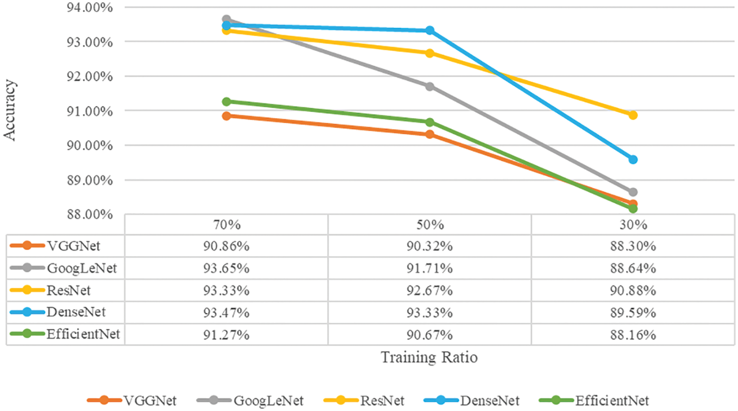
Figure 13: Classification accuracy for each model trained by datasets containing contour images
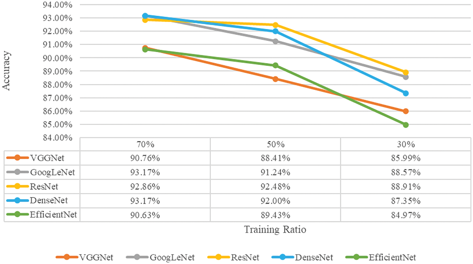
Figure 14: Classification accuracy for each model trained by original datasets
4.2 Experimental Results and Analysis of Hierarchical Ensembles
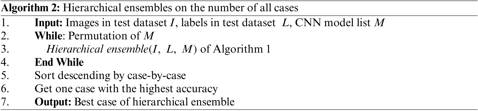
The hierarchical ensemble architecture in Fig. 12 shows that the central model has the greatest influence. Therefore, the best performance model is centered. We then deploy the second-best performing model in the second position and the third-best performing model in the fourth position. Finally, the lower two models with poor performance were placed in the first and fifth places. We judged that performing hierarchical ensembles in this way would have the best performance. The results of performing a hierarchical ensemble on the number of cases in which the trained individual models can be deployed demonstrate the validity of the above hypothesis. The experimental method for the number of cases is presented in Algorithm 2.
Tab. 3 shows the results of the hierarchical ensemble experiment for each scenario, and Fig. 15 shows a visual representation of the results of the hierarchical ensemble experiment. As a result of performing the hierarchical ensemble, it was confirmed that the performance was improved in all scenarios, and higher accuracy was achieved when the contour image was learned than when it was not learned. Comparing the average accuracy of the overall model by scenario with the accuracy of the hierarchical ensemble, the accuracy improvement was not significant when the ratio of training data was high; however, the lowest ratio of training data (scenario 6) achieved a performance improvement of up to 4.68%. Therefore, the data insufficient constraint problem can be solved if the hierarchical ensemble is used when the data required for deep learning model training is insufficient.
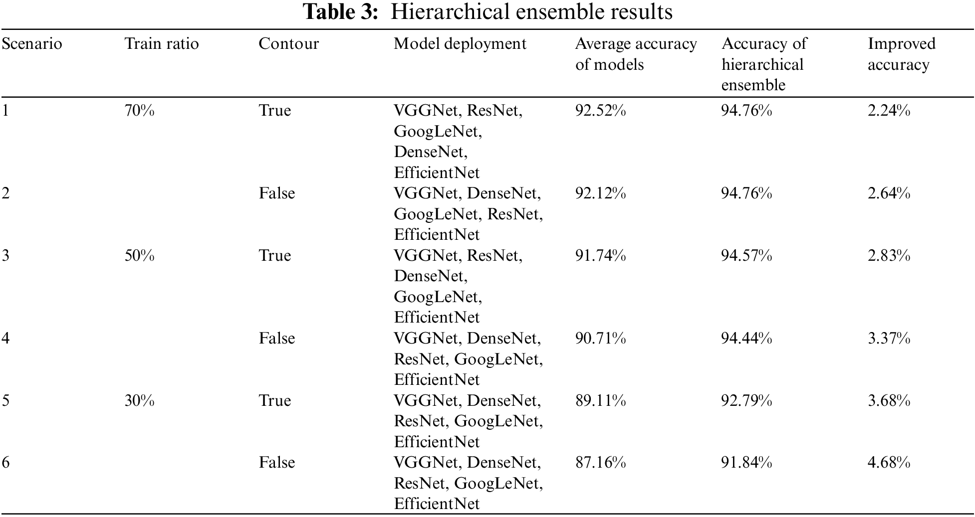
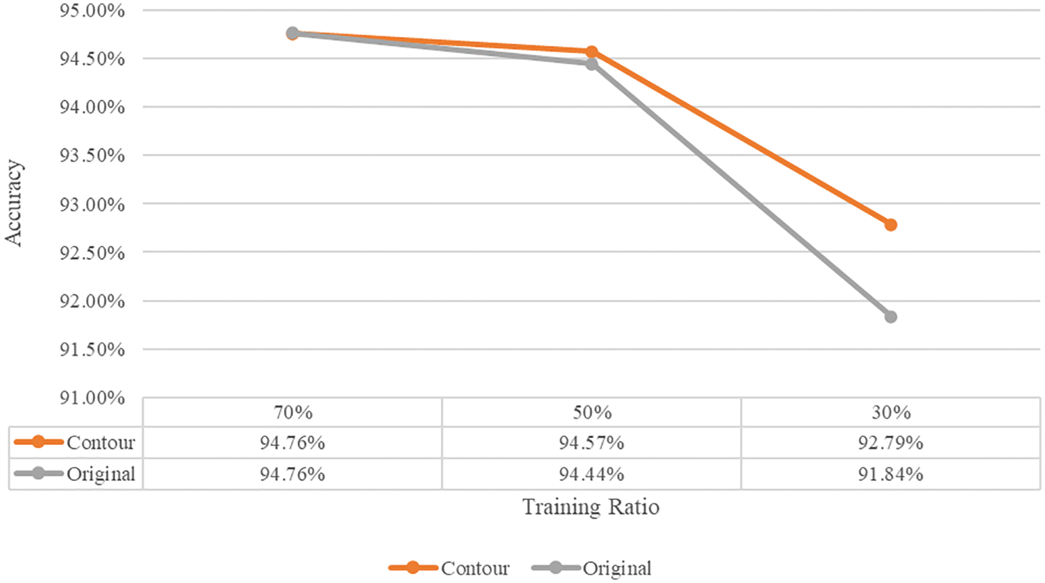
Figure 15: Visualization of hierarchical ensemble results
Tab. 4 presents the performance comparison of the basic and hierarchical ensembles. Fig. 16 shows the performance comparison of the basic ensemble and the hierarchical ensemble when the contour image is trained, and Fig. 17 shows the visualization of the performance comparison between the basic ensemble and the hierarchical ensemble when the contour image is not trained. First, a basic ensemble trains five CNN models, such as a hierarchical ensemble. We derived the predicted values for each model to perform a basic ensemble. The average of each derived model prediction was used to calculate the accuracy of the image. Although there were some performance improvements for basic ensembles, we found that hierarchical ensembles had an average performance improvement of 1.84% over basic ensembles and achieved up to 2.41% when training data had the lowest ratio (Scenario 6).
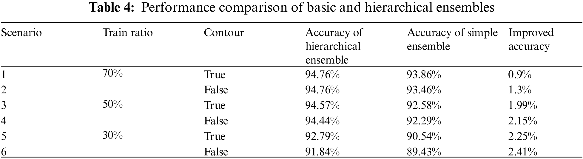

Figure 16: Performance comparison of basic and hierarchical ensembles trained by datasets containing contour images
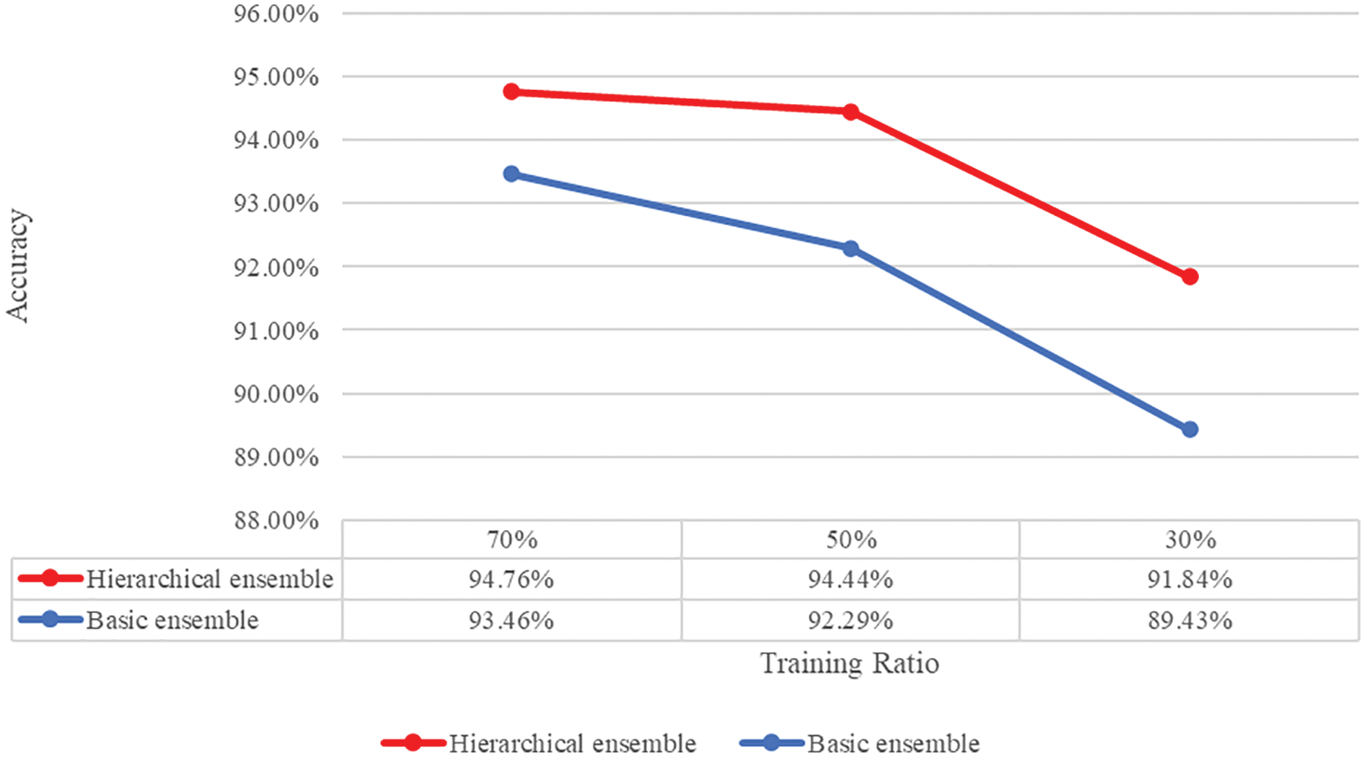
Figure 17: Performance comparison of basic and hierarchical ensembles–trained by original datasets
In this study, six scenarios were set according to the ratio of training data and whether the contour image was trained, and land use data were individually trained on well-known pretrained neural networks such as VGGNet, GoogLeNet, ResNet, DenseNet, and EfficientNet. A hierarchical ensemble was performed for all cases in which each learned model could be deployed. As a result, we not only confirmed that the contour image was a significant factor in the performance of deep learning models but also achieved high classification accuracy with small amounts of training data through hierarchical ensembles. Further studies related to optimization, such as hyperparameter tuning of each CNN model, are required to achieve the best accuracy, as the purpose of the proposed method is to demonstrate the importance of contour image learning and improve the classification performance of the model through hierarchical ensembles. In future studies, we expect to identify and extract significant features among features extracted from each model and further improve the model training speed and accuracy through a combination of multiple models.
Funding Statement: The authors received no specific funding for this study.
Conflicts of Interest: The authors declare that they have no conflicts of interest to report regarding this study.
1. D. G. Lowe, “Distinctive image features from scale-invariant keypoints,” International Journal of Computer Vision, vol. 60, no. 2, pp. 91–110. 2004. [Google Scholar]
2. N. Dalal and B. Triggs, “Histograms of oriented gradients for human detection,” in 2005 IEEE Computer Society Conf. on Computer Vision and Pattern Recognition (CVPR'05), San Diego, CA, USA, vol. 1, pp. 886–893, 2005. [Google Scholar]
3. M. D. Kumar, M. Babaie, S. Zhu, S. Kalra and H. R. Tizhoosh, “A comparative study of CNN, BoVW and LBP for classification of histopathological images,” in Proc. IEEE Symp. Series on Computational Intelligence, Honolulu, HI, USA, pp. 1–7, 2017. [Google Scholar]
4. Y. LeCun, B. Boser, J. S. Denker, D. Henderson, R. E. Howard et al., “Backpropagation applied to handwritten zip code recognition,” Neural Computation, vol. 1, no. 4, pp. 541–551, 1989. [Google Scholar]
5. Y. LeCun, L. Bottou, Y. Bengio and P. Haffner, “Gradient-based learning applied to document recognition,” in Proc. IEEE, vol. 86, no. 11, pp. 2278–2324, 1998. [Google Scholar]
6. A. Krizhevsky, I. Sutskever and G. E. Hinton, “Imagenet classification with deep convolutional neural networks,” Advances in Neural Information Processing Systems, vol. 25, pp. 1097–1105, 2012. [Google Scholar]
7. X. Lv, D. Ming, Y. Chen and M. Wang, “Very high resolution remote sensing image classification with SEEDS-CNN and scale effect analysis for superpixel CNN classification,” International Journal of Remote Sensing, vol. 40, no. 2, pp. 506–531, 2019. [Google Scholar]
8. K. Simonyan and A. Zisserman, “Very deep convolutional networks for large-scale image recognition,” 2014. [Online]. Available: https://arxiv.org/abs/1409.1556. [Google Scholar]
9. C. Szegedy, W. Liu, Y. Jia, P. Sermanet, S. Reed et al., “Going deeper with convolutions,” in Proc. the IEEE Conf. on Computer Vision and Pattern Recognition, Boston, MA, pp. 1–9, 2015. [Google Scholar]
10. K. He, X. Zhang, S. Ren and J. Sun, “Deep residual learning for image recognition,” in Proc. the IEEE Conf. on Computer Vision and Pattern Recognition, Las Vegas, NV, USA, pp. 770–778, 2016. [Google Scholar]
11. G. Huang, Z. Liu, L. Van Der Maaten and K. Q. Weinberger, “Densely connected convolutional networks,” in Proc. the IEEE Conf. on Computer Vision and Pattern Recognition, Honolulu, HI, USA, pp. 4700–4708, 2017. [Google Scholar]
12. M. Tan and Q. Le, “Efficientnet: Rethinking model scaling for convolutional neural networks,” 2019. [online]. Available: https://arxiv.org/abs/1905.11946. [Google Scholar]
13. A. Aziz, M. Attique, U. Tariq, Y. Nam, M. Nazir et al., “An ensemble of optimal deep learning features for brain tumor classification,” Computers, Materials & Continua, vol. 69, no. 2, pp. 2653–2670, 2021. [Google Scholar]
14. P. W. Khan and Y. Byun, “Adaptive error curve learning ensemble model for improving energy consumption forecasting,” Computers, Materials & Continua, vol. 69, no. 2, pp. 1893–1913, 2021. [Google Scholar]
15. A. Majid, M. A. Khan, Y. Nam, U. Tariq, S. Roy et al., “COVID19 classification using CT images via ensembles of deep learning models,” Computers, Materials & Continua, vol. 69, no. 1, pp. 319–337, 2021. [Google Scholar]
16. N. K. Seerangan and S. V. Shanmugam, “Ensemble based temporal weighting and Pareto ranking (ETP) model for effective root cause analysis,” Computers, Materials & Continua, vol. 69, no. 1, pp. 819–830, 2021. [Google Scholar]
17. S. M. Alotaibi, A. M. I. Basheer and M. A. Khan, “Ensemble machine learning based identification of pediatric epilepsy,” Computers, Materials & Continua, vol. 68, no. 1, pp. 149–165, 2021. [Google Scholar]
18. H. Kutlu and E. Avcı, “A novel method for classifying liver and brain tumors using convolutional neural networks, discrete wavelet transform and long short-term memory networks,” Sensors, vol. 19, no. 9, 2019. [Google Scholar]
19. F. Özyurt, “A fused CNN model for WBC detection with MRMR feature selection and extreme learning machine,” Soft Computing, vol. 24, no. 11, pp. 8163–8172, 2020. [Google Scholar]
20. H. Kutlu, E. Avci and F. Özyurt, “White blood cells detection and classification based on regional convolutional neural networks,” Medical Hypotheses, vol. 135, 2020. [Google Scholar]
21. O. A. Penatti, K. Nogueira, J. A. Dos Santos, “Do deep features generalize from everyday objects to remote sensing and aerial scenes domains?,” in Proc. the IEEE Conf. on Computer Vision and Pattern Recognition workshops, Boston, MA, USA, pp. 44–51, 2015. [Google Scholar]
22. Y. Yang and S. Newsam, “Bag-of-visual-words and spatial extensions for land-use classification,” in Proc. the 18th SIGSPATIAL Int. Conf. on Advances in Geographic Information Systems, San Jose California, pp. 270–279, 2010. [Google Scholar]
23. J. Bouvrie, “Notes on convolutional neural networks,” 2006. [online]. Available: http://cogprints.org/5869/. [Google Scholar]
24. A. G. Howard, M. Zhu, B. Chen, D. Kalenichenko, W. Wang et al., “Mobilenets: Efficient convolutional neural networks for mobile vision applications,” 2017. [online]. Available: https://arxiv.org/abs/1704.04861. [Google Scholar]
25. X. Zhang, X. Zhou, M. Lin and J. Sun, “ShuffleNet: An extremely efficient convolutional neural network for mobile devices,” in Proc. the IEEE Conf. on Computer Vision and Pattern Recognition, Salt Lake City, UT, USA, pp. 6848–6856. 2018. [Google Scholar]
26. M. E. Sobel, “Asymptotic confidence intervals for indirect effects in structural equation models,” Sociological Methodology, vol. 13, pp. 290–312, 1982. [Google Scholar]
27. A. K. Cherri and M. A. Karim, “Optical symbolic substitution: Edge detection using Prewitt, Sobel, and Roberts operators,” Applied Optics, vol. 28, no. 21, pp. 4644–4648, 1989. [Google Scholar]
28. G. T. Shrivakshan and C. Chandrasekar, “A comparison of various edge detection techniques used in image processing,” International Journal of Computer Science Issues (IJCSI), vol. 9, no. 5, pp. 269–276, 2012. [Google Scholar]
29. J. Canny, “A computational approach to edge detection,” IEEE Transactions on Pattern Analysis and Machine Intelligence, vol. PAMI-8, no. 6, pp. 679–698, 1986. [Google Scholar]
30. D. P. Kingma and J. Ba, “Adam: A method for stochastic optimization,” 2014. [online] Available: https://arxiv.org/abs/1412.6980. [Google Scholar]
 | This work is licensed under a Creative Commons Attribution 4.0 International License, which permits unrestricted use, distribution, and reproduction in any medium, provided the original work is properly cited. |