DOI:10.32604/cmc.2022.022901
| Computers, Materials & Continua DOI:10.32604/cmc.2022.022901 | |
| Article |
Deep-piRNA: Bi-Layered Prediction Model for PIWI-Interacting RNA Using Discriminative Features
1Department of Computer Science, Abdul Wali Khan University Mardan, Khyber Pakhtunkhwa, 23200, Pakistan
2Department of Information Technology, University of Haripur, Khyber Pakhtunkhwa, 22620, Pakistan
3Faculty of Science, Universiti Putra Malaysia, UPM Serdang, 43400, Malaysia
*Corresponding Author: Mohd Amiruddin Abd Rahman. Email: mohdamir@upm.edu.my
Received: 22 August 2021; Accepted: 11 November 2021
Abstract: Piwi-interacting Ribonucleic acids (piRNAs) molecule is a well-known subclass of small non-coding RNA molecules that are mainly responsible for maintaining genome integrity, regulating gene expression, and germline stem cell maintenance by suppressing transposon elements. The piRNAs molecule can be used for the diagnosis of multiple tumor types and drug development. Due to the vital roles of the piRNA in computational biology, the identification of piRNAs has become an important area of research in computational biology. This paper proposes a two-layer predictor to improve the prediction of piRNAs and their function using deep learning methods. The proposed model applies various feature extraction methods to consider both structure information and physicochemical properties of the biological sequences during the feature extraction process. The outcome of the proposed model is extensively evaluated using the k-fold cross-validation method. The evaluation result shows that the proposed predictor performed better than the existing models with accuracy improvement of 7.59% and 2.81% at layer I and layer II respectively. It is anticipated that the proposed model could be a beneficial tool for cancer diagnosis and precision medicine.
Keywords: Deep neural network; DNC; TNC; CKSNAP; PseDPC; cancer discovery; Piwi-interacting RNAs; Deep-piRNA
PiWi-interacting Ribonucleic acids (piRNAs) are a unique class of small non-coding RNA (sncRNA) molecules that express in a variety of human somatic cells and also in animal cells [1]. The piRNA molecule contains 19-33 nucleotides which is slightly different from small interfering RNA and micro-RNA molecules in length [2]. So over 1.5 million unique piRNA molecules have been discovered in fruit flies which are clustered in thousands of genomic loci [3]. In addition, the piRNA molecules have been discovered in rats, mice, fish, mammals and somatic tissues [4]. It has been reported that the piRNA molecules play an important role in many gene functions such as translation of specific proteins, regulate gene expression, fight against viral infection, maintain genome integrity and transposon silencing etc. [5,6]. In addition, the piRNA molecules move within the genome and induce mutations, insertions, and deletions which may cause genome instability [7]. Moreover, many studies (e.g., [8–11]) have shown that the occurrence of piRNAs are related with multiple tumor types and actively involved for the cancer cells development and progression. Hence, there is a great interest in identification and classification of piRNA molecules and their function types for cancer cells diagnosis and therapy, drug development and gene stability. Owing to the importance of the piRNA molecules in the genome, the prediction and identification of piRNA molecules has become an important research area in computational biology [12,13].
In the literature numerous computational models have been proposed for the identification of piRNAs and non-piRNA sequences using machine learning algorithms. For example, Zhang et al. [14] developed a k-mer based piRNA-predictor and Wang et al. [15] developed a piRNA annotation program that predicts piRNAs sequence based on SVM as a learning algorithm. Luo et al. [16] and Li et al. [17] demonstrated an ensemble approach for prediction of piRNA and non-piRNA molecules using physicochemical properties. Recently, Wang et al. [18] proposed a convolutional neural network based computational method for identification of piRNA molecules. The authors employed k-mer (k = 1 to 5) for sequence. It is worth mentioning that these models have ignored whether these piRNAs molecules are functional and non-functional piRNA molecules or non-functional piRNA. To identify piRNAs and their functions, Liu et al. [19] proposed a 2L-piRNA ensemble predictor and employed PseKNC method to extract a feature vector along with the physicochemical properties. Similarly, Chen et al. [20] developed an SVM-based predictor called piRNAPred for prediction of piRNA and their function type. The piRNAPred utilized sequence information along with structure information i.e., physicochemical properties to represent RNAs sequence into a feature vector. Both the models have yielded promising results in term of accuracy; however, these models are developed based on traditional machine learning algorithms which are unable to accurately predict the piRNAs sequences and their function types due to a high similarity between piRNAs and non-piRNAs. In addition, these models require a huge amount of human expertise and capability to extract the predominant features [21,22].
Recently, Khan et al. proposed two different computational models known as 2L- piRNADNN [23] and piRNA (2L)-PseKNC [24] for the identification of piRNA and their function using multi-layer deep neural network algorithms. Both the models have produced promising results in term of performance. However, the 2L- piRNADNN model use a simple dinucleotide auto covariance (DAC) method and the piRNA (2L)-PseKNC model employs different modes of pseudo K-tuple nucleotide composition (PseKNC) method using different values for K (i.e., K = 1, 2, 3) feature extraction which ignored global sequence order information.
In this paper, we propose a powerful and robust multi-layers deep neural network (DNN) model [25] based on Chou’s 5-steps rule [26]. The proposed deep-piRNA model is constructed to improve the prediction accuracy of piRNAs and their functions. The framework of the proposed model is depicted in Fig. 1, where firstly, the deep-piRNA employs four different feature extraction methods such as normalized moreau-broto autocorrelation (NMBroto), Z curve parameters for frequencies of phase independent di-nucleotides (Z_curve_12bit), dinucleotide composition (DNC) and single nucleotide composition (SNC) to formulate RNAs sequence into features vectors. Secondly, a composite feature vector is constructed by combining all the features vectors. Finally, the DNN algorithm is applied as a prediction engine to build the proposed computational model. The deep-piRNA performance is extensively evaluated using rigorous K-fold cross validation tests. The experimental results show that the proposed model outperformed the existing prediction models in terms of accuracy and other performance measurements parameters. It is anticipated that the proposed technique could be a useful tool for cancer diagnosis and drug development.
The remainder of the paper is structured as follows: Section 2 explains the material and methods, which includes the benchmark dataset and feature extraction, and classification algorithms. The performance evaluation metrics are presented in Section 3. Section 4 discusses the experimental findings and discussions. Finally, Section 5 includes the paper conclusion and future work.
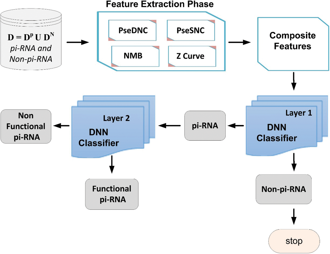
Figure 1: Framework of the proposed model
According to Chou comprehensive review [27,28] a valid and reliable benchmark dataset is always required for the design of a powerful and robust computational model. Hence, in this paper we used the same benchmark datasets that were used in [17,19]. The selected datasets can be expressed in mathematical form using Eqs. (1) and (2):
where
where
In machine learning, extracting all the relevant details from the RNA sequence which includes the sequence ordering information and main structural characteristics is a very crucial and important step. The efficiency of any proposed algorithm largely depends on how efficiently relevant information is derived from the raw data which are the RNA samples in our case. Selection of a suitable feature extraction technique leads to an optimized model which can yield precise predictions with the selection of most favorable features [35,36]. These RNA sequences must be translated into the form of a vector or discrete model because the classifier works and understands the discrete form, not the sequences /samples directly [37]. Consider now the second rule of Chou’s 5-step guidelines, in this paper we utilize four different feature extraction techniques i.e., NMBroto, Z curve-12bit, SNC and DNC. The explanation of these feature extraction methods is in the following section.
The Z Curve is a 3-Dimensional (i.e.,
where
2.2.2 Normalized Moreau Broto (NMB) Method
Normalized Moreau Broto autocorrelation method is a type of topological feature encoder, also known as a molecular connectivity index, that expresses the degree of correlation between two nucleotides, in terms of their structural or physicochemical properties. The normalized Moreau Broto autocorrelation method is widely used in studies [38,39] and defined in Eq. (6).
where, j indicates descriptor,
2.2.3 Pseudo K-Tuple Nucleotide Composition (PseKNC)
PseKNC is one of the feature formulation methods which is widely applied in computational biology for the formulation of RNA / DNA sequences [40,41]. In this paper, we have applied the PseKNC to formulate the RNA sequence in the form of a discrete feature vector. Using two values of K (i.e., PseSNC (Ƙ = 1) and PseDNC (Ƙ = 2)). In PseSNC, RNA sequence is expressed with the single nucleotides and gives 4-D while in PseDNC RNA sequence is expressed with the help of two consecutive nucleotides pairs and gives 16-D [42]. It can be numerically expressed as:
where, T symbol represents the transpose operator.
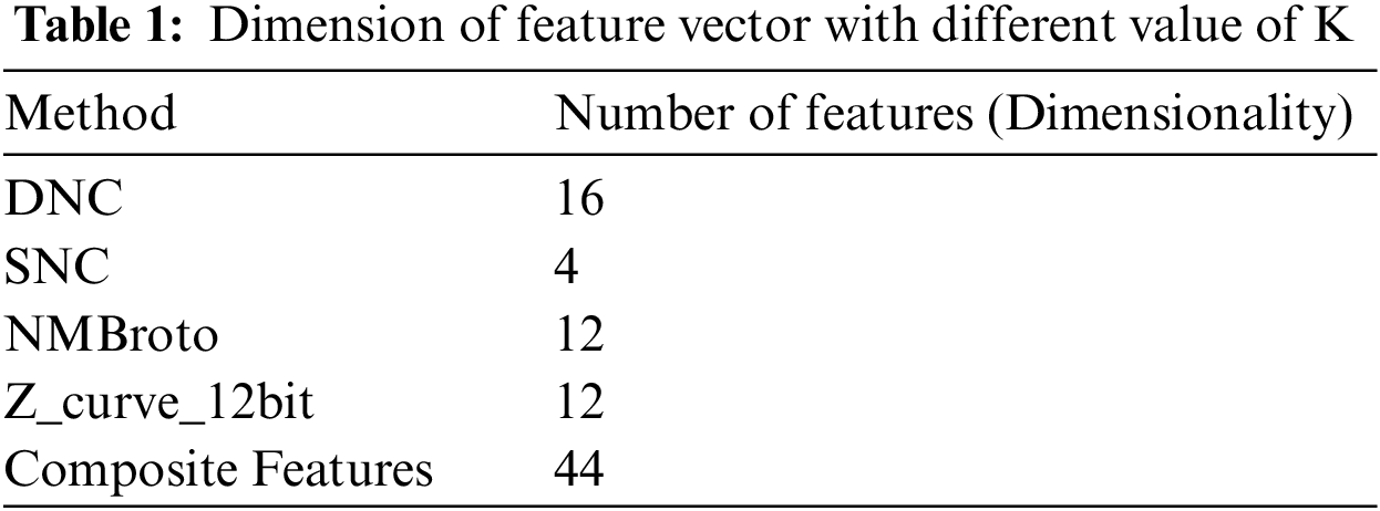
The proposed Deep-piRNA model utilizes four different feature extraction techniques i.e., PseSNC, PseDNC, Normalized Moreau Broto autocorrelation, and Z curve to represent the RNA sequences. Tab. 1 shows the number of features obtained for each method. Using Eq. (5), we have merged all four feature vectors (i.e., Eqs. (5) and (6) & Eqs. (8) and (9)) to create a composite feature vector.
2.4 Deep Neural Network Architecture
DNN is a subfield of machine learning algorithms in artificial intelligence that is inspired by the human brain working mechanism and its activities [43]. A DNN model topology consists of an input layer, output layer and multiple hidden layers as shown in Fig. 2. The hidden layers are important elements of the DNN model and are actively engaged in the process of learning [44]. Using more hidden layers in the model training process may increase the model efficiency, however, it may arise problems such as computational cost, model complexity and overfitting [45]. The main characteristic of the DNN model is automatically extracting appropriate features from the specified unlabeled or unstructured dataset without requiring human engineering and experience using standard learning methods [46]. Several researchers have proved that the DNN model worked better than the traditional learning methods used for various complex classification problems [47]. In addition, the DNN model has been successfully applied in many areas including bio-engineering [48], image recognition [49], speech recognition [50] and natural language processing [51].
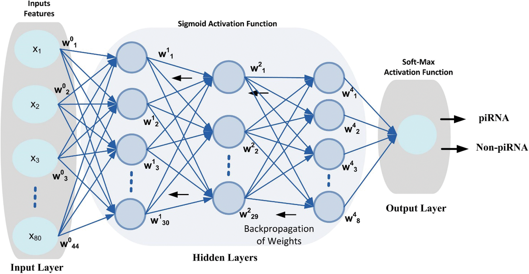
Figure 2: DNN configuration topology, the circle represents neurons at each layer
Inspired from the successful implementation of the deep learning models in various domains for complex classification problems, this paper considered the DNN model for the prediction of simulation sites using benchmark dataset. The proposed DNN model is configured with 3-hidden layers along with input layer and output layer as shown in Fig. 3. Each layer in the DNN topology is configured with multiple neurons that process the input features vector and produce output using Eq. (11). The weight matrix on every neuron is initialized using Xavier function [52] which has the ability to remain the variance same through each layer. Moreover, a back propagation technique is applied to update the weight matrix in such a way that errors between the output class and target class are minimized. Nonlinear activation function i.e., Sigmoid is applied at input layer and at hidden layers. The activation function helps the model to learn non-linearity and complex patterns in a dataset. Moreover, it determines either a neuron can be fired or ignored depending upon the output produced by the particular neuron [53]. Additionally, a softmax activation function is applied at the output layer that generated a value in the range of [0,1] that represent the probability of data-point belong to a particular class.
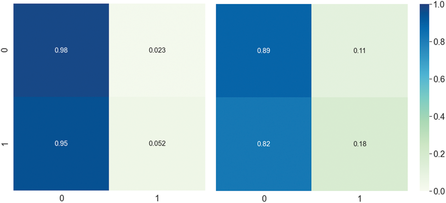
Figure 3: DNN model Confusion matrix using composite features. The left side represents the first layer confusion matrix, and the right side represents the second layer confusion matrix
where
3 Performance Evaluation Metrics
The efficiency of a machine learning system can be measured using various assessment criteria. Here, we adopt commonly used metrics to assess our proposed Deep-piRNA model performance that include accuracy (ACC), Specificity (Sp), Sensitivity (Sn), AUC score represent the area under the ROC curve and Matthew’s Correlation Coefficient (Mcc) [54–56]. In order to make these measures more straightforward and easier to understand, we used the method suggested in the number of publications [57,58] which is based on the Chou symbol and definition [59]. These metrics using the Chou symbol are defined as:
where, T+ symbolizes true positives,
Accuracy (Acc) shows the overall Accuracy of a model. Sensitivity and Specificity are inversely proportional. So, when we increase sensitivity, there is a decrease in specificity and vice versa. In order words lower the threshold we get more positive values, so the sensitivity increases and the specificity decreases. So, when we raise the threshold, we get more negative values, so we get more specificity and less sensitivity. MCC gives accurate concordant ratings for a prediction that accurately identifies both positive and negative. The area under the ROC curve is a graphical plot between false positive rate (FPR = 1 - specificity) and true positive rate (TPR = sensitivity). Here, we find the AUC to be the key criterion for measuring success independent of any threshold.
The proposed Deep-piRNA efficiency is evaluated and discussed in depth in this section. We have used the Windows 10 operating system along with Java 8 and Python 3.7 to evaluate the proposed algorithm. First, through an empirical process, we discuss the optimization of proposed model hyper-parameters. Second, the proposed model performance was evaluated using different feature extraction techniques. Thirdly, we compare the performance with other classifiers. Fourthly, we analyze the proposed model using an independent dataset. Finally, we compare the performance with existing predictors.
4.1 Hyper-Parameters Optimization
The DNN configuration topology includes several parameters, and such parameters are referred to as hyper-parameters. The hyper-parameters include hidden layers, weight initialization, learning rate, process optimization methods, activation functions and configuration of various numbers of neurons in each layer. The model hyper-parameters must be tuned before the learning process begins [25] as the efficiency of the DNN model is mainly based on the optimum configuration of the hyper-parameters. The commonly used hyper-parameters are shown in Tab. 2.
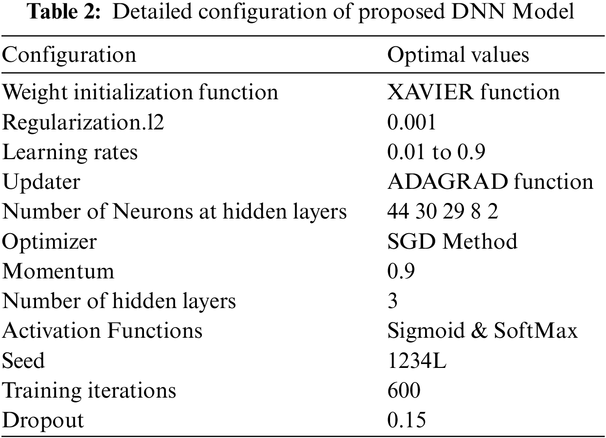
The grid search technique was used to tune the hyper-parameters configuration to obtain the optimal value for the DNN model. The grid search technique automatically evaluates the performance of the proposed model for every combination of parameters. First, we performed a few experiments to find optimum configuration values for the learning rate and activation function. Secondly, we obtain optimized values for the number of training iterations through several experiments. The optimum values of the various hyper-parameters are shown in Tab. 2.
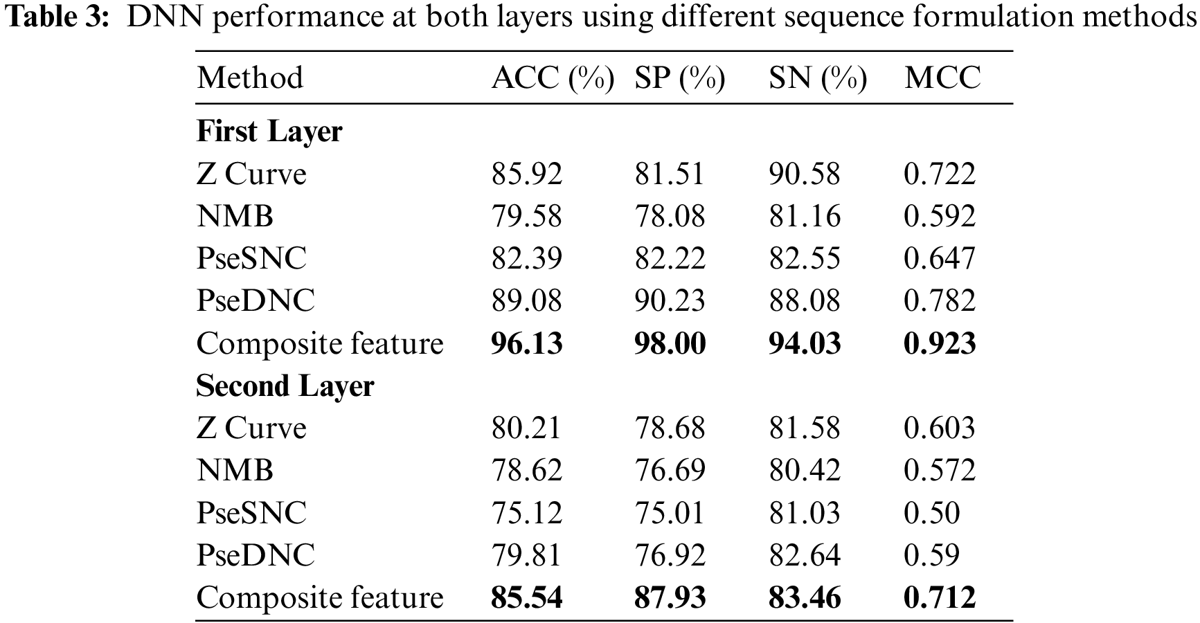
The DNN model's predictive performance was evaluated using different vector feature extraction techniques i.e., PseSNC, PseDNC, Normalized Moreau Broto Autocorrelation and Z curve and composite features. In the literature, there are several methods listed that can be applied to test a classification model's efficiency and effectiveness. These include jackknife, independent dataset and cross-validation test (sub-sampling test) [56]. In this paper we used a cross-validation test, i.e., 10-fold cross-validation test and independent dataset test to check the DNN model's performance. It should be noted that we designed the DNN model with hyperparameters configuration values provided in Tab. 2 during the performance evaluation.
The prediction performance achieved by the DNN model using different feature vectors at the first and second layer is shown in Tab. 3. The table reveals that the best performance obtained by the DNN model utilizes composite features vector relative to the individual type of extraction of features on both layers. For instance, The DNN model obtained a significantly improved average accuracy of 96.13%, sensitivity 94.03%, specificity 98.00% and MCC 0.923 on composite features vector in the first layer. Similarly, from Tab. 3 the best performance obtained by the DNN model in the second layer achieved an accuracy of 85.54%, sensitivity 83.46%, specificity 87.46% and MCC 0.712. Additionally, a confusion matrix is presented in Fig. 3 to further explore the behavior of the proposed DNN in prediction using the composite features vector.
4.3 Comparison with other Machine Learning Methods
Here, we use composite feature vectors to compare the performance of the DNN model with other traditional machine learning classifiers. The classifiers we considered for the performance analysis included: Random Forest (RF) [60], K-Nearest Neighbor (KNN) [61] , Support-Vector-Machine (SVM) [62]. Tab. 4 demonstrates the performance comparison between various classifiers at both layers.
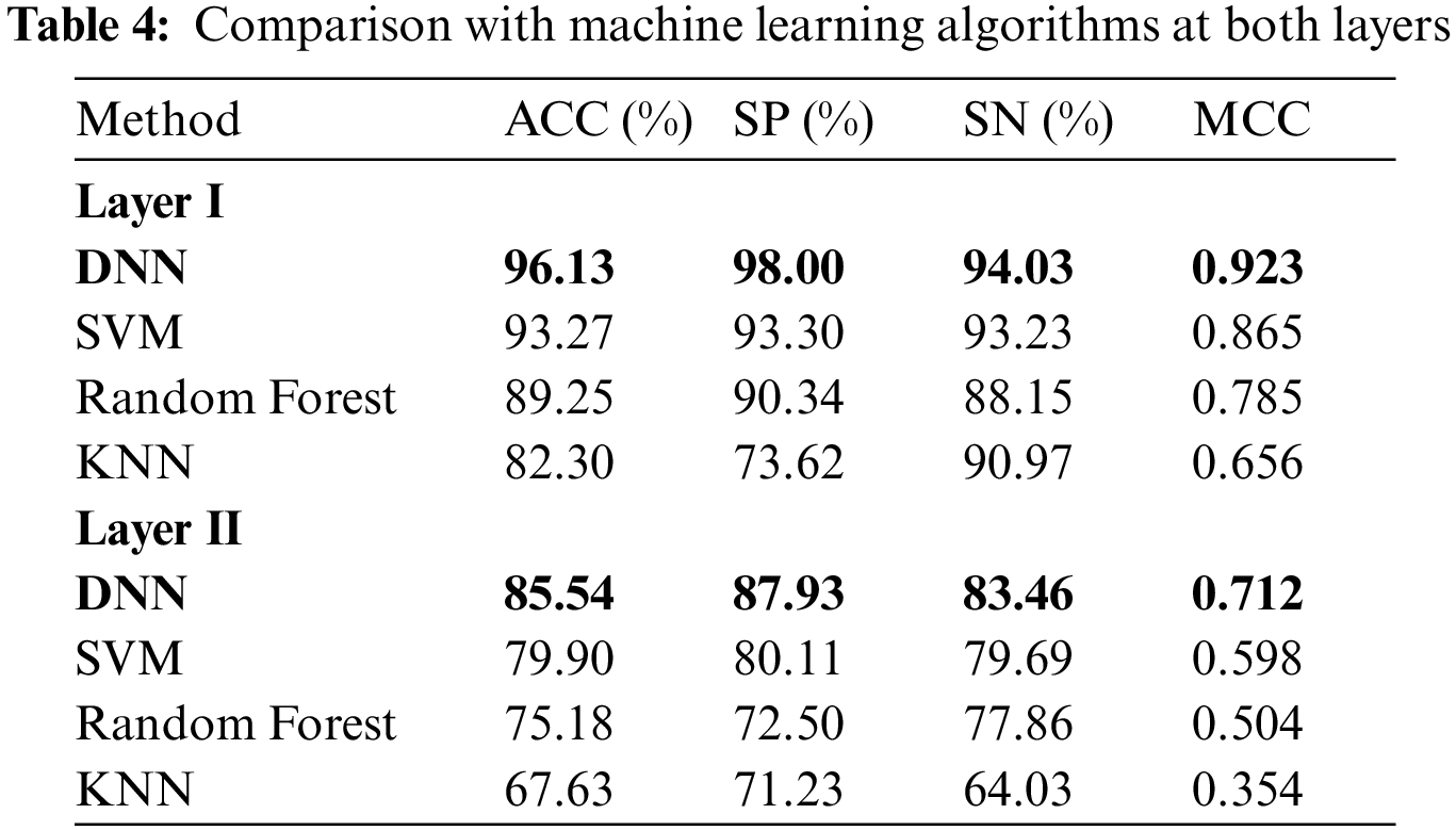
It is shown from Tab. 4 that the DNN model attained the most distinguished accuracies in the first and second layers i.e., 96.13% and 85.54% respectively compared with other classifiers. Moreover, DNN using the composite feature set attained an effective MCC i.e., 0.923% and 0.712 respectively in the first and second layer. On the other hand, after examining traditional classifiers performance; SVM on composite feature set did perform satisfactorily and obtained an accuracy of 93.27%, with a specificity of 93.23%, sensitivity value of 93.30%, and MCC of 0.86 as compared to KNN and RF. Therefore, in this paper, the proposed model adopted the DNN as the final classifier.
4.4 Analysis of Learning Hypotheses Using Independent Dataset
To ensure the stability and reliability of the proposed model we perform an independent dataset test. The output findings of the S2 independent dataset are shown in Tab. 5. From the Tab. 5, it is illustrated that evaluating the composite feature set on different classifiers, the proposed DNN classifier performed remarkably and achieved accuracy 93.53% in the first layer. Moreover, the proposed DNN classifiers recorded the highest sensitivity of 95.89% among all other classifiers and achieved the highest specificity of 90.91%. Furthermore, the SVM on composite feature set performed well and reported second highest accuracy and MCC i.e., 90.59 and 0.811 respectively in the first layer.

However, composite features set in conjunction with DNN performed extraordinarily more than any of the individual feature sets and reported 81.90% accuracy and 0.637 of MCC in the second layer. At last, the composite space features have performed better in sensitivity and specificity i.e., 80.37% and 83.33% respectively that indicates that the success rates reached by the suggested predictor are quite high.
4.5 Comparison with Existing Models
Here, we compare our proposed model with the existing benchmark methods i.e., [16,17,19,20,23], in the first and second layer respectively. The mentioned latest methods build prediction models based on machine learning algorithms. The performance of our proposed model and the existing benchmark models are evaluated on benchmark datasets by using 10-fold cross-validation. For facilitating comparison, Tab. 6 shows the corresponding results obtained by the existing state of the art methods.

It can be observed from Tab. 6 that our proposed Deep-piRNA model performs overwhelmingly better than the existing model. Our proposed new predictor Deep-piRNA achieved the highest accuracy of 96.13% and 85.54% and Matthew’s correlation coefficient (MCC) 0.923 and 0.712 in both layers respectively. These two most important metrics reflect the overall performance, robustness, and stability of the proposed predictor. The proposed method also yields much better performances in specificity (Sp) and sensitivity (Sn) comparable with the existing methods i.e., 98.00% and 94.03% in the first layer and 87.93% and 83.46% in the second layer respectively. The average accuracy improvements in both layers i.e., 7.59% and 2.81% respectively illustrate the significance of the proposed model and self-evident compared with existing predictors.
Furthermore, we have adopted the graphical analysis to show the usefulness of our proposed Deep-piRNA model, as it is mostly useful and shown in recent studies of complicated biological systems [63,64]. The value of the receiver operating characteristic (ROC) Curve field reflects the model's efficiency so that the higher the value the better the output [65,66]. Fig. 4 shows the graph of the area under the ROC curve (AUC). As we can see from Fig. 4, the proposed classifier is remarkably larger i.e., 0.983 and 0.878 in both the first and second layers respectively. This indicates that there are 98% and 88% expectations that the model will be able to distinguish between positive and negative classes in both layers. The intuitive graphical approach demonstrates the merit and virtue of our proposed Deep-piRNA model.
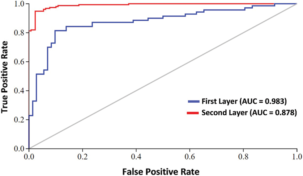
Figure 4: AUC at first layer and second layer using composite features
The present study showed high performance for the detection of piRNA and their function. The proposed two-layer predicator is a robust and accurate predictor and can be used for diagnosis of numerous tumor types of cancer and drug development. We used different methods for sequence encoding and then fused to construct a more efficient representation of the given input space. The performance of the two-layer predictor was investigated on different classifiers. The results shows that optimized DNN classifier algorithm outperformed existing state of the art models with accuracy improvement of 7.59% and 2.81% at layer I and layer II respectively. In future work, we have planned to design a web server that can access and utilize the proposed model. Finally, it is anticipated that Deep-piRNA is a useful tool and that will help the research community in precision medicine, drug development, and cancer cell diagnosis. In addition, it is evident that a huge amount of genome data is generated due to advancement in next-generation sequencing technology which poses computational challenges for sequential computing approaches. In future work, we plan to apply parallel programming techniques to parallelize computations on few processing nodes.
Acknowledgement: The authors would like to thank the Ministry of Higher Education Malaysia (MOHE) and Universiti Putra Malaysia for supporting the project.
Funding Statement: This research was supported by the Ministry of Higher Education (MOHE) of Malaysia through Fundamental Research Grant Scheme (FRGS/1/2020/ICT02/UPM/02/3).
Conflicts of Interest: The authors declare that they have no conflicts of interest to report regarding the present study.
Source Code and Benchmark Dataset: The proposed model source code and benchmark dataset are available at https//www.github.com/salman-khan-mrd/piRNA-2L-pseKNC.
1. F. Khan, M. Khan, N. Iqbal, S. Khan, D. Muhammad Khan et al., “Prediction of recombination spots using novel hybrid feature extraction method via deep learning approach,” Frontiers in Genetics, vol. 11, no. 539227, pp. 1–15, 2020. [Google Scholar]
2. A. Aravin, D. Gaidatzis, S. Pfeffer, M. Lagos-Quintana, P. Landgraf et al., “A novel class of small RNAs bind to MILI protein in mouse testes,” Nature, vol. 442, no. 7099, pp. 203–207, 2006. [Google Scholar]
3. N. Wynant, D. Santos and J. Vanden Broeck, “Biological mechanisms determining the success of rna interference in insects,” International Review of Cell and Molecular Biology, vol. 312, no. Suppl., pp. 139–167, 2014. [Google Scholar]
4. A. Sarkar and Z. Ghosh, “Rejuvenation of piRNAs in emergence of cancer and other diseases,” in AGO-Driven Non-Coding RNAs: Codes to Decode the Therapeutics of Diseases. Cambridge, MA, USA: Academic Press, pp. 319–333, 2019. [Google Scholar]
5. D. N. Cox, A. Chao, J. Baker, L. Chang, D. Qiao et al., “A novel class of evolutionarily conserved genes defined by piwi are essential for stem cell self-renewal,” Genes and Development, vol. 12, no. 23, pp. 3715–3727, 1998. [Google Scholar]
6. C. Klattenhoff and W. Theurkauf, “Biogenesis and germline functions of piRNAs,” Development, vol. 135, no. 1, pp. 3–9, 2007. [Google Scholar]
7. S. Houwing, L. M. Kamminga, E. Berezikov, D. Cronembold, A. Girard et al., “A role for piwi and pirnas in germ cell maintenance and transposon silencing in zebrafish,” Cell, vol. 129, no. 1, pp. 69–82, 2007. [Google Scholar]
8. Y. Mei, D. Clark and L. Mao, “Novel dimensions of piRNAs in cancer,” Cancer Letters, vol. 336, no. 1, pp. 46–52, 2013. [Google Scholar]
9. J. Cheng, H. Deng, B. Xiao, H. Zhou, F. Zhou et al., “PiR-823, a novel non-coding small RNA, demonstrates in vitro and in vivo tumor suppressive activity in human gastric cancer cells,” Cancer Letters, vol. 315, no. 1, pp. 12–17, 2012. [Google Scholar]
10. M. Moyano and G. Stefani, “PiRNA involvement in genome stability and human cancer,” Journal of Hematology and Oncology, vol. 8, no. 1, pp. 38, 2015. [Google Scholar]
11. A. Hashim, F. Rizzo, G. Marchese, M. Ravo, R. Tarallo et al., “RNA sequencing identifies specific PIWI-interacting small noncoding RNA expression patterns in breast cancer,” Oncotarget, vol. 5, no. 20, pp. 9901–9910, 2014. [Google Scholar]
12. N. C. Lau, A. G. Seto, J. Kim, S. Kuramochi-Miyagawa, T. Nakano et al., “Characterization of the piRNA complex from rat testes,” Science, vol. 313, no. 5785, pp. 363–367, 2006. [Google Scholar]
13. S. T. Grivna, E. Beyret, Z. Wang and H. Lin, “A novel class of small RNAs in mouse spermatogenic cells,” Genes and Development, vol. 20, no. 13, pp. 1709–1714, 2006. [Google Scholar]
14. Y. Zhang, X. Wang and L. Kang, “A k-mer scheme to predict piRNAs and characterize locust piRNAs,” Bioinformatics, vol. 27, no. 6, pp. 771–776, 2011. [Google Scholar]
15. K. Wang, C. Liang, J. Liu, H. Xiao, S. Huang et al., “Prediction of piRNAs using transposon interaction and a support vector machine,” BMC Bioinformatics, vol. 15, no. 1, pp. 419, 2014. [Google Scholar]
16. L. Luo, D. Li, W. Zhang, S. Tu, X. Zhu et al., “Accurate prediction of transposon-derived pirnas by integrating various sequential and physicochemical features,” PLoS ONE, vol. 11, no. 4, pp. e0153268, 2016. [Google Scholar]
17. D. Li, L. Luo, W. Zhang, F. Liu and F. Luo, “A genetic algorithm-based weighted ensemble method for predicting transposon-derived piRNAs,” BMC Bioinformatics, vol. 17, no. 1, pp. 329, 2016. [Google Scholar]
18. K. Wang, J. Hoeksema and C. Liang, “piRNN: Deep learning algorithm for piRNA prediction,” PeerJ, vol. 6, no. 8, pp. e5429, 2018. [Google Scholar]
19. B. Liu, F. Yang and K. C. Chou, “2L-piRNA: A two-layer ensemble classifier for identifying piwi-interacting rnas and their function,” Molecular Therapy - Nucleic Acids, vol. 7, no. W1, pp. 267–277, 2017. [Google Scholar]
20. Y. Chen, T. Li, R. Song, Q. Yin and M. Gao, “Support vector machine classifier for accurate identification of pirna,” Applied Sciences, vol. 8, no. 11, pp. 1–9, 2018. [Google Scholar]
21. N. Inayat, M. Khan, N. Iqbal, S. Khan, M. Raza et al., “iEnhancer-DHF: Identification of enhancers and their strengths using optimize deep neural network with multiple features extraction methods,” IEEE Access, vol. 9, pp. 40783–40796, 2021. [Google Scholar]
22. A. Ahmad, S. Akbar, S. Khan, M. Hayat, F. Ali et al., “Deep-AntiFP: Prediction of antifungal peptides using distanct multi-informative features incorporating with deep neural networks,” Chemometrics and Intelligent Laboratory Systems, vol. 208, no. 104214, pp. 1–10, 2021. [Google Scholar]
23. S. Khan, M. Khan, N. Iqbal, T. Hussain, S. A. Khan et al., “A two-level computation model based on deep learning algorithm for identification of pirna and their functions via chou’s 5-steps rule,” International Journal of Peptide Research and Therapeutics, vol. 26, no. 2, pp. 795–809, 2020. [Google Scholar]
24. S. Khan, M. Khan, N. Iqbal, S. A. Khan and K. C. Chou, “Prediction of piRNAs and their function based on discriminative intelligent model using hybrid features into Chou’s PseKNC,” Chemometrics and Intelligent Laboratory Systems, vol. 203, no. 104056, pp. 1–10, 2020. [Google Scholar]
25. S. Khan, M. Khan, N. Iqbal, M. Li and D. M. Khan, “Spark-based parallel deep neural network model for classification of large scale rnas into pirnas and non-pirnas,” IEEE Access, vol. 8, pp. 136978–136991, 2020. [Google Scholar]
26. A. Majid, M. M. Khan, N. Iqbal, M. A. Jan, M. M. Khan et al., “Application of parallel vector space model for large-scale dna sequence analysis,” Journal of Grid Computing, vol. 17, no. 2, pp. 313–324, 2019. [Google Scholar]
27. K. C. Chou, “Some remarks on protein attribute prediction and pseudo amino acid composition,” Journal of Theoretical Biology, vol. 273, no. 1, pp. 236–247, 2011. [Google Scholar]
28. K. C. Chou and H. B. Shen, “REVIEW : Recent advances in developing web-servers for predicting protein attributes,” Natural Science, vol. 1, no. 2, pp. 63–92, 2009. [Google Scholar]
29. P. Zhang, X. Si, G. Skogerb, J. Wang, D. Cui et al., “piRBase: A web resource assisting piRNA functional study,” Database: The Journal of Biological Databases and Curation, vol. 2014, no. bau110, pp. 1–7, 2014. [Google Scholar]
30. D. Bu, K. Yu, S. Sun, C. Xie, G. Skogerb et al., “NONCODE v3.0: Integrative annotation of long noncoding RNAs,” Nucleic Acids Research, vol. 40, no. D1, pp. D210–D215, 2012. [Google Scholar]
31. L. Fu, B. Niu, Z. Zhu, S. Wu, W. Li et al., “Accelerated for clustering the next-generation sequencing data,” Bioinformatics, vol. 28, no. 23, pp. 3150–3152, 2012. [Google Scholar]
32. J. Jia, Z. Liu, X. Xiao, B. Liu and K. C. chou, “iPPBS-Opt: A sequence-based ensemble classifier for identifying protein-protein binding sites by optimizing imbalanced training datasets,” Molecules, vol. 21, no. 1, pp. 95, 2016. [Google Scholar]
33. J. Jia, Z. Liu, X. Xiao, B. Liu and K. C. Chou, “iSuc-PseOpt: Identifying lysine succinylation sites in proteins by incorporating sequence-coupling effects into pseudo components and optimizing imbalanced training dataset,” Analytical Biochemistry, vol. 497, no. 6, pp. 48–56, 2016. [Google Scholar]
34. C. Xie, J. Yuan, H. Li, M. Li, G. Zhao et al., “NONCODEv4: Exploring the world of long non-coding RNA genes,” Nucleic Acids Research, vol. 42, no. D1, pp. D98–D103, 2014. [Google Scholar]
35. Y. Saeys, I. Inza and P. Larrañaga, “A review of feature selection techniques in bioinformatics,” Bioinformatics, vol. 23, no. 19, pp. 2507–2517, 2007. [Google Scholar]
36. I. Iguyon and A. Elisseeff, “An introduction to variable and feature selection,” Journal of Machine Learning Research, vol. 3, pp. 1157–1182, 2003. [Google Scholar]
37. K. C. Chou, “Impacts of bioinformatics to medicinal chemistry,” Medicinal Chemistry, vol. 11, no. 3, pp. 218–234, 2015. [Google Scholar]
38. Z. P. Feng and C. T. Zhang, “Prediction of membrane protein types based on the hydrophobic index of amino acids,” Journal of Protein Chemistry, vol. 19, no. 4, pp. 269–275, 2000. [Google Scholar]
39. F. Ali, S. Ahmed, Z. N. K. Swati and S. Akbar, “DP-BINDER: Machine learning model for prediction of DNA-binding proteins by fusing evolutionary and physicochemical information,” Journal of Computer-Aided Molecular Design, vol. 33, no. 7, pp. 645–658, 2019. [Google Scholar]
40. H. Lin, E. Z. Deng, H. Ding, W. Chen and K. C. Chou, “iPro54-PseKNC: A sequence-based predictor for identifying sigma-54 promoters in prokaryote with pseudo k-tuple nucleotide composition,” Nucleic Acids Research, vol. 42, no. 21, pp. 12961–12972, 2014. [Google Scholar]
41. W. Chen, P. M. Feng, H. Lin and K. C. Chou, “Chou, iSS-PseDNC: Identifying splicing sites using pseudo dinucleotide composition,” BioMed Research International, vol. 2014, no. 623149, pp. 1–12, 2014. [Google Scholar]
42. Z. Liu, X. Xiao, W. R. R. Qiu and K. C. C. Chou, “iDNA-Methyl: Identifying DNA methylation sites via pseudo trinucleotide composition,” Analytical Biochemistry, vol. 474, no. Suppl., pp. 69–77, 2015. [Google Scholar]
43. N. Tishby and N. Zaslavsky, “Deep learning and the information bottleneck principle,” in IEEE Information Theory Workshop (ITW). Jerusalem, Israel, 1–5, 2015. [Google Scholar]
44. Y. Wu, H. Tan, L. Qin, B. Ran and Z. Jiang, “A hybrid deep learning based traffic flow prediction method and its understanding,” Transportation Research Part C: Emerging Technologies, vol. 90, no. 2554, pp. 166–180, 2018. [Google Scholar]
45. D. Ravi, C. Wong, F. Deligianni, M. Berthelot, J. Andreu-Perez et al., “Deep learning for health informatics,” IEEE Journal of Biomedical and Health Informatics, vol. 21, no. 1, pp. 4–21, 2017. [Google Scholar]
46. S. Min, B. Lee and S. Yoon, “Deep learning in bioinformatics,” Briefings in Bioinformatics, vol. 18, no. 5, pp. 851–869, 2017. [Google Scholar]
47. J. Ma, R. P. Sheridan, A. Liaw, G. E. Dahl and V. Svetnik, “Deep neural nets as a method for quantitative structure-activity relationships,” Journal of Chemical Information and Modeling, vol. 55, no. 2, pp. 263–274, 2015. [Google Scholar]
48. Z. Zhu, E. Albadawy, A. Saha, J. Zhang, M. R. Harowicz et al., “Deep learning for identifying radiogenomic associations in breast cancer,” Computers in Biology and Medicine, vol. 109, no. 3, pp. 85–90, 2019. [Google Scholar]
49. A. Krizhevsky, I. Sutskever and G. E. Hinton, “ImageNet classification with deep convolutional neural networks,” Communications of the ACM, vol. 60, no. 6, pp. 84–90, 2017. [Google Scholar]
50. G. Hinton, L. Deng, D. Yu, G. E. Dahl, A. R. Mohamed et al., “Deep neural networks for acoustic modeling in speech recognition: The shared views of four research groups,” IEEE Signal Processing Magazine, vol. 29, no. 6, pp. 82–97, 2012. [Google Scholar]
51. A. Bordes, S. Chopra, J. Weston, S. Chopra and J. Weston, “Question answering with subgraph embeddings,” in Proc. of the 2014 Conf. on Empirical Methods in Natural Language Processing (EMNLP), Doha, Qatar, pp. 615–620, 2014. [Google Scholar]
52. X. Glorot and Y. Bengio, “Understanding the difficulty of training deep feedforward neural networks,” in Proc. of the Thirteenth Int. Conf. on Artificial Intelligence and Statistics, Sardinia, Italy, pp. 249–256, 2010. [Google Scholar]
53. T. Voisin, P. Rouet-Benzineb, N. Reuter and M. Laburthe, “Orexins and their receptors: structural aspects and role in peripheral tissues,” Cellular and Molecular Life Sciences (CMLS), vol. 60, no. 1, pp. 72–87, 2003. [Google Scholar]
54. J. Chen, H. Liu, J. Yang and K. C. Chou, “Prediction of linear B-cell epitopes using amino acid pair antigenicity scale,” Amino Acids, vol. 33, no. 3, pp. 423–428, 2007. [Google Scholar]
55. Y. Guo, L. Yu, Z. Wen and M. Li, “Using support vector machine combined with auto covariance to predict protein-protein interactions from protein sequences,” Nucleic Acids Research, vol. 36, no. 9, pp. 3025–3030, 2008. [Google Scholar]
56. M. F. Sabooh, N. Iqbal, M. Khan, M. Khan and H. F. Maqbool, “Identifying 5-methylcytosine sites in RNA sequence using composite encoding feature into Chou’s PseKNC,” Journal of Theoretical Biology, vol. 452, pp. 1–9, 2018. [Google Scholar]
57. Y. Xu, J. Ding, L. Y. Wu and K. C. Chou, “iSNO-PseAAC: Predict cysteine s-nitrosylation sites in proteins by incorporating position specific amino acid propensity into pseudo amino acid composition,” PLoS ONE, vol. 8, no. 2, pp. 1–7, 2013. [Google Scholar]
58. W. Chen, P. M. Feng, H. Lin and K. C. Chou, “IRSpot-PseDNC: Identify recombination spots with pseudo dinucleotide composition,” Nucleic Acids Research, vol. 41, no. 6, pp. 1–9, 2013. [Google Scholar]
59. K. K. C. Chou, “Using subsite coupling to predict signal peptides,” Protein Engineering Design and Selection, vol. 14, no. 2, pp. 75–79, 2001. [Google Scholar]
60. K. Fawagreh, M. M. Gaber and E. Elyan, “Random forests: From early developments to recent advancements,” Systems Science and Control Engineering, vol. 2, no. 1, pp. 602–609, 2014. [Google Scholar]
61. S. Akbar, S. Khan, F. Ali, M. Hayat, M. Qasim et al., “iHBP-DeepPSSM: Identifying hormone binding proteins using PsePSSM based evolutionary features and deep learning approach,” Chemometrics and Intelligent Laboratory Systems, vol. 204, no. 104103, pp. 1–11, 2020. [Google Scholar]
62. S. Yue, P. Li and P. Hao, “SVM classification: Its contents and challenges,” Applied Mathematics-A Journal of Chinese Universities, vol. 18, no. 3, pp. 332–342, 2003. [Google Scholar]
63. G. P. Zhou and M. H. Deng, “An extension of Chou’s graphic rules for deriving enzyme kinetic equations to systems involving parallel reaction pathways,” Biochemical Journal, vol. 222, no. 1, pp. 169–176, 1984. [Google Scholar]
64. K. C. Chou and S. Forsén, “Graphical rules for enzyme-catalysed rate laws,” Biochemical Journal, vol. 187, no. 3, pp. 829–835, 1980. [Google Scholar]
65. I. W. Althaus, A. J. Gonzales, J. J. Chou, D. L. Romero, M. R. Deibel et al., “The quinoline U-78036 is a potent inhibitor of HIV-1 reverse transcriptase,” Journal of Biological Chemistry, vol. 268, no. 20, pp. 14875–14880, 1993. [Google Scholar]
66. G. P. Zhou, D. Chen, S. Liao and R. B. Huang, “Recent progresses in studying helix-helix interactions in proteins by incorporating the wenxiang diagram into the NMR spectroscopy,” Current Topics in Medicinal Chemistry, vol. 16, no. 6, pp. 581–590, 2015. [Google Scholar]
 | This work is licensed under a Creative Commons Attribution 4.0 International License, which permits unrestricted use, distribution, and reproduction in any medium, provided the original work is properly cited. |