Computers, Materials & Continua DOI:10.32604/cmc.2022.022993
Article

Intelligent Dynamic Inversion Controller Design for Ball and Beam System

Ibrahim M. Mehedi1,2,*, Abdulah Jeza Aljohani1,2, Md Mottahir Alam1, Mohamed Mahmoud3, Mohammed J. Abdulaal1, Muhammad Bilal1,2 and Waleed Alasmary4

1Department of Electrical and Computer Engineering (ECE), King Abdulaziz University, Jeddah, 21589, Saudi Arabia
2Center of Excellence in Intelligent Engineering Systems (CEIES), King Abdulaziz University, Jeddah, 21589, Saudi Arabia
3Electrical and Computer Engineering, Electrical and Computer Engineering, TN, 38505, United States
4Computer and Information Systems, Umm Al-Qura University, Makkah, Saudi Arabia
*Corresponding Author: Ibrahim M. Mehedi. Email: imehedi@kau.edu.sa
Received: 25 August 2021; Accepted: 20 December 2021

Abstract: The Ball and beam system (BBS) is an attractive laboratory experimental tool because of its inherent nonlinear and open-loop unstable properties. Designing an effective ball and beam system controller is a real challenge for researchers and engineers. In this paper, the control design technique is investigated by using Intelligent Dynamic Inversion (IDI) method for this nonlinear and unstable system. The proposed control law is an enhanced version of conventional Dynamic Inversion control incorporating an intelligent control element in it. The Moore-Penrose Generalized Inverse (MPGI) is used to invert the prescribed constraint dynamics to realize the baseline control law. A sliding mode-based intelligent control element is further augmented with the baseline control to enhance the robustness against uncertainties, nonlinearities, and external disturbances. The semi-global asymptotic stability of IDI control is guaranteed in the sense of Lyapunov. Numerical simulations and laboratory experiments are carried out on this ball and beam physical system to analyze the effectiveness of the controller. In addition to that, comparative analysis of RGDI control with classical Linear Quadratic Regulator and Fractional Order Controller are also presented on the experimental test bench.

Keywords: Ball and beam system (BBS); unstable system; internal model; PD controllers; IDI control; robust control

1  Introduction

The ball and beam system (BBS) is a standard laboratory experimental setup and serves as an essential benchmark to investigate and validate the performance of various control strategies [1]. The tilt angle of the beam is the most significant action through which the ball position is controlled systematically by varying the tilt angle. It is an under-actuated open-loop unstable system having two degrees of freedom. The fundamental idea of BBS can be applied to a wide range of applications such as stabilizing the aircraft in its horizontal position while landing, tanker on-road carrying liquid, aircraft yaw roll control, goods handling problem by industrial robots, etc.

The control of an under-actuated system is an active research field having fewer control inputs than the state variables that need to be controlled. The experimental setup of BBS deals with the two loops control strategy. The outer loop is responsible for ball position control, whereas the inner loop is engaged for servo angle control. Due to its double loop control strategies, it is not easy to control this system using linear controllers [2]. Therefore, several control techniques are proposed in the literature to investigate the tracking and stabilization problem of BBS [3–5].

A feedback linearization method is applied for BBS, which produces singularity and does not produce good results [3]. A Fuzzy-based controller is investigated in [6], showing the tracking performance numerically without implementing it on a practical testbed. The Fuzzy and Neural Networks based algorithms are presented in [7,8]. The robust control technique based on the sliding mode approach is also investigated for the ball balancing problem, see [9,10]. A Backstepping controller is designed in [11] to simulate the tracking problem of BBS. An anti-windup compensator (AWC) control scheme is also demonstrated in [12]. Similarly, the optimal performance of Model Predictive Control (MPC) is investigated to evaluate the tracking characteristics for ball and beam equipment [5].

Recent work was proposed designing a controller comprising two embedded loops based on linear fractional-order calculus [2]. The outer-loop and inner-loop control the ball's location on the beam and angle of servo gear, respectively. The prime focus of this method of control is to demonstrate a fractional-order control scheme to enhance efficiency, which is reported in several journals [13–17]. However, the performance is unsatisfactory because an integer order traditional controller is related to the non-integer order integrator, which is used in the outer loop.

In addition to that, Nonlinear Dynamic Inversion (NDI) was also implemented for this ball and beam underactuated system, see [18]. However, this control method requires the exact model of the plant dynamics.

Therefore, NDI control may possess certain shortcomings and limitations while developing the algorithms. This includes the simplified approximations to introduce the inverse model of plant dynamics, square dimensionality condition, useful nonlinearity cancellations, etc.

Recently a control law focused on the inversion principle is proposed known as Generalized Dynamic Inversion (GDI), which addresses the limitations of the classical NDI approach [19]. The control objectives of GDI are defined in the form of differential state constraints which are calculated along the solution paths of the system dynamics. The control law is obtained by inverting the suggested constraints using Moore-Penrose Generalized Inverse (MPGI) [20]. Further, the GDI algorithm is made intelligent by augmenting the switching term based on the concept of classical SMC principle to ensure robustness against parametric uncertainties and un-modeled dynamics while guaranteeing semi-global asymptotic stability conditions [21–25].

A two-loop control architecture is employed in this paper to solve the tracking and stabilization problem for two degrees of freedom under actuated BBS. A proportional derivative (PD) control is implemented in the outer loop to generate rotary servo angle commands based on the ball position on the beam. An intelligent version of GDI, Intelligent Dynamic Inversion (IDI), is used to process the inner loop's angular command. Identical (baseline) control and switching (continuous) control elements make up this IDI control system. The baseline control enforces the constraint dynamics based on the deviation function of the rotary servo angle for stable attitude tracking, while the switching control ensures robustness against nonlinearities and external perturbations. As a result, the proposed control guaranteed a semi-global attitude tracking system and bounded tracking errors. Quanser's BBS is used to simulate and perform laboratory experiments on the controller performance and compare the controller performance to existing control strategies.

The remaining sections of the paper are described as follows. The modeling of BBS is presented in Section 2. The two-loop control structure is discussed in Section 3. The classical PD control design for the outer position loop is presented in Section 4. The design implementation of IDI control for tracking the servo angle command is given in Section 5. The detailed stability analysis that will guarantee semi-global asymptotic stability was illustrated in Section 6. Controller validation through computer simulations and experimental findings are reported in Sections 7 and 8. Finally, the concluding remarks are given in Section 9.

2  Description of BBS

Quanser developed BBS, a benchmark laboratory test bench [1], to validate control algorithms that are defined relative degrees with nonlinear attributes. The two significant ball and beam setup components are the ball and beam unit and rotary servo unit. One end of the finite length beam is fixed by a shaft, whereas the other end is connected to the rotary servo unit, as shown in the schematic diagram in Fig. 1. Therefore, this unstable architecture is well known as an open-loop system in control technology. The core objective is to orient and stabilize the ball placed on the beam according to the commanded reference input profile. In Fig. 1, x is the linear displacement ball, mbis the mass, rbis the beam's radius, and Jbis the ball's momentum, respectively. The relative angle of the beam concerning the horizontal plane is denoted by α, whereas the gravitational acceleration is mentioned by g. The expression of the linear acceleration of the ball is given as Eq. (1).

x¨(t)=mbgsin⁡α(t)rb2mbrb2+Jb(1)

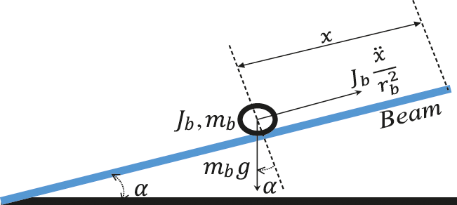
Figure 1: Ball and beam system

Similarly, the relation between the beam angle α and servo angle θl(t) is expressed as

sin⁡α(t)=sin⁡θl(t)rarmLbeam(2)

where Lbeamis the length of the beam and rarmis the gap between the rotary servo output gear and the coupled joint. To relate the linear displacement x with the rotary servo angle θ, place the expression of sinα(t) in the linear acceleration equation given by Eq. (2), it implies

x¨(t)=mbgθl(t)rarmrb2Lbeam(mbrb2+Jb)(3)

The second major component of the ball and beam setup is the rotary servo base unit which comprises a DC motor with a gearbox, as shown in Fig. 2. The subscript m represents the motor attributes in the given schematic, whereas l characterizes the load shaft variables. In the rotary servo unit, the resistance is denoted by R, L is the inductance, ω is the angular speed, τ is the applied torque, J is the moment of inertia, and B stands for the viscous friction. The variable ebrepresents the back-electromotive voltage, where kmis the back-emf constant. To realize the dynamical model of the rotary servo unit, the mechanical and electrical systems are combined to form the relationship between the angular speed of the motor load shaft ωland the applied controlled voltage Vm. The dynamical system is represented by the following equations

θ˙l=ωl(4)

ω˙lJeq+Beqvωl=AmVm(t)(5)

where the equivalent moment of inertia Jeqis expressed as

Jeq=ηgkg2Jm+Jl(6)

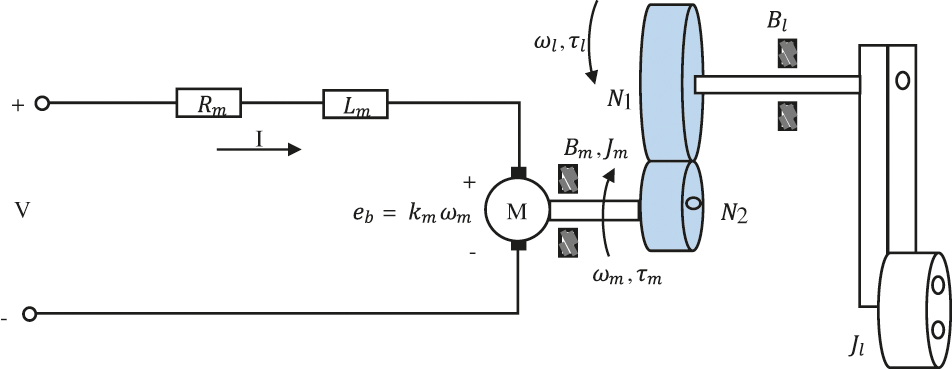
Figure 2: Rotary servo unit

and the equivalent damping term Beqvis given by

Beqv=ηgkg2ηmktkm+BeqRmRm(7)

In the expressions of the equivalent moment of inertia and damping, ηgand ηmrepresent the efficiency of the gearbox and motor, respectively. The motor torque constant is denoted by kt,and kgis the gear ratio. The actuator gain Amis computed as

Am=ηgkgηmktRm(8)

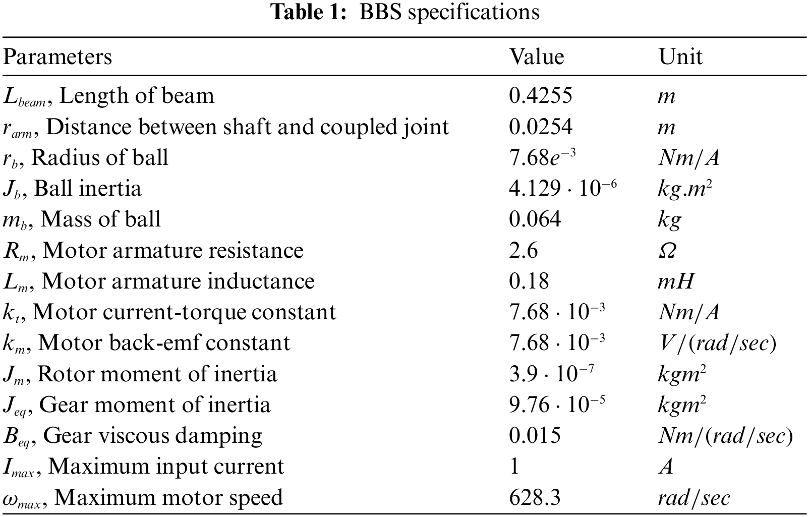
The numerical value of the BBS parameters is listed in Tab. 1, see [1,26].

3  Cascade Control Architecture

A cascade control architecture based on the time separation principle is proposed to control the ball's position on the beam, as shown in Fig. 3. Based on the measured ball position x, the outer positional loop computes the desired angle θldof the servo load shaft by engaging the classical PD control. The inner fast attitude loop incorporates IDI control to track the desired angle θldby generating the corresponding motor controlled voltage V such that the desired ball position on the beam is achieved in minimal time.

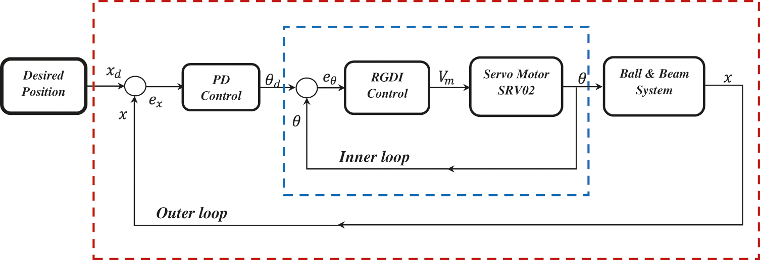
Figure 3: Cascade control architecture

4  Outer Loop PD Control Design

Given the desired and actual ball's position, i.e., xdand x, the classical PD controller is engaged in the outer loop to generate the desired servo angle command θldfor the inner loop to minimize the positional error of the ball placed on the beam. The asymptotically stable virtual (desired) dynamics to compute θldbased on the positional error of the ball in the horizontal plane is expressed as

kd(x˙−x˙d)+kp(x−xd)=θld(9)

where kpand kdare controller gains chosen to calculate the suitable value of θldsuch that x approached xdin minimum time. It is noteworthy to mention here that the position feedback of the ball is acquired from an analog sensor with its inherent noise. By taking its derivative, it will generate an amplified high-frequency signal transmitted to the inner loop via feedback which causes the grinding noise in the motor. The derivative is replaced by a first-order filter governed following dynamics to compensate for this effect.

H(s)=ωfss+ωf(10)

where ωfrepresents the cutoff frequency, whose value is set to be 6.28 rad/s.

5  Attitude Control Using IDI

This section discussed the design and implementation of IDI control for attitude control of the rotary servo unit of BBS. The proposed non-square inversion-based intelligent controller proves to be an efficient and effective control strategy to deal with complex nonlinear systems. The control law comprises two major components, i.e., an equivalent or baseline control and a switching control component. The general form of IDI control law is expressed as follows

uIDI=ueq+urbt(11)

The first component ueqrepresents the baseline controller, which enforces the prescribed constraint dynamics based on the attitude deviation function for stable attitude tracking. On the other hand, urbtrepresents the discontinuous control element whose design principle is based on the classical SMC approach to address robustness against uncertain dynamics, parametric variations, and external disturbances.

5.1 Baseline Control Design

The equations of motion of rotary servo unit angular rate dynamics given by Eq. (5) is expressed as

ω˙l=F+GVm(12)

where F=Jeq−1Beqvωl, G=Jeq−1Am, and Vm represent the controlled voltage. The design is initiated by determining two constraint differential equations based on the attitude deviation function, which implies

ζ¨θl+c1ζ˙θl+c2ζθl=0(13)

ζ˙ωl+c3ζωl=0(14)

where ζθl=x1eθl2=x1(θl−θld)2 and ζωl=x2eωl2=x2(ωl−ωld)2 are the deviation functions and ωl is the angular speed. The order of the constraint equation is equal to the relative degree of the respective controlled variable. The coefficients c1, c2, and c3 are selected such that the characteristic polynomials are given by Eqs. (13), and (14) is Hurwitz, such that ζθl→0 and ζωl→0 as t→∞ [19]. Computing and substituting the time derivatives in the constraint dynamics given by Eqs. (13) and (14) yields the following under-determined equivalent algebraic system.

[A1A2]Vm=[B1B2]⇒AVm=B(15)

where the elements of the controls coefficient column vector function A:Rn×[t0,∞)→R2×1 is given by

A1=2x1eθlG

A2=2x2eωlG

and the elements of the controls load vector function B:Rn×[t0,∞)→R2×1 are given as

B1=2x1eθlω˙ld−2x1e˙θl2−2x1eθlF−2c1x1eθle˙θl−c2x1eθl2

B2=2x2eωlω˙ld−2x2eωlF−c3x2eωl2

The baseline or equivalent controlled voltage Vmeq is computed by inverting the algebraic system given by Eq. (15) using MPGI yields the following expression

Vmeq=A+B+Pλ(16)

where A+ represents the MPGI of A defined as

A+={ATA}−1AT(17)

Remark 1: The matrix A2×1 appeared to be a tall matrix, which causes the value of P to become zero by using the property of pseudo-inverse A+A=1. Hence the under-determined nature of constraint dynamics does not qualify with the benefit of the null control vector due to the ineffectiveness of the null projection matrix. Hence, the null control is supposed to be incompetent and not considered in the present control design methodology.

5.2 Switching Control Design

A suitable discontinuous control element is determined to solve the reachability problem, which ensures robustness against parametric uncertainties, system nonlinearities, and external disturbances. The resultant GDI-SMC or IDI control law is constructed to be of the following form

Vm=Vmeq−A+Ks∥s∥

Vm=A+B−A+Ks∥s∥(18)

where s=[sθlsωl]T is an appropriate switching surface vector, whose vector elements are defined as

sθl=ξ˙θl+c1ξθl+c2∫⁡ξθldt(19)

sωl=ξωl+c3∫⁡ξωldt(20)

Moreover, K is 2×2 diagonal gain matrix with positive valued diagonal elements k1 and k2, ensuring that the sliding mode dynamics are maintained and attained. Therefore, the controlled voltage Vm given by the Eq. (18) is reasonably competent to attract the sliding surfaces given by Eqs. (19) and (20) and enforce the system trajectories to slide along the sliding surfaces.

6  Stability Analysis

The time derivatives of the sliding surfaces are evaluated as

s˙θl=ξ¨θl+c1ξ˙θl+c2ξθl(21)

s˙ωl=ξ˙ωl+c3ξωl(22)

It has been observed that the asymptotic convergence of the sliding surfaces sθl and sωl to zero implies the asymptotic realization of the constraint dynamics given by the Eqs. (13) and (14), and its equivalent algebraic form given by Eq. (15). Hence, the sliding vector s is defined as

s˙=AVm−B(23)

To prove the asymptotic convergence of the error dynamics, place the control law Vm given by Eq. (18) in sliding mode dynamics given by Eq. (23), resulting in

s˙=A{A+B−A+Ks∥s∥}−B

={AA+−I2×2}B−A+Ks∥s∥(24)

Consider the following positive definite Lyapunov candidate function

V=12sTs(25)

The time derivative of V is computed as

V˙=sTs˙=sT{(AA+−I2×2)B−AA+Ks∥s∥}

=sT{AA+−I2×2)}B−sTAA+Ks∥s∥(26)

The 2-(induced) norms of AA+ and AA+−I2×2 are unity. It follows that V˙≤0 is guaranteed if σmin(K)>∥B(x(0),0)∥, where σmin is the minimum singular value function. Moreover, because V˙=0 occurs only at s=02, it follows Lassale's principle [27] that s=02 is attractive. Moreover, the discontinuous term in the right-hand side of Eq. (26) implies that this condition on K guarantees finite-time convergence of s and s˙ to the zero vectors, which implies asymptotic convergence of eθl and eωl to zero. Finally, because it is assumed that the matrix gain K can be increased arbitrarily such that the stability condition is satisfied for any initial state condition, it follows that the design guarantees semi-global asymptotic stability of (eθl,e˙θl)=(eωl,e˙ωl)=(0,0).

7  Numerical Simulation

This section investigates the performance of IDI control law through computer simulations on the dynamical simulator of BBS developed by considering the model of ball and beam unit given by Eq. (3) and the model of rotary servo unit given by Eqs. (4) and (5). The simulation environment is created in Simulink/Matlab, in which the closed-loop performance is evaluated by commanding the square wave profile having an amplitude of ±20m with 0.05Hz frequency, assuming nominal system parameters. The initial condition of the system state vector is set as [xx˙θlθ˙lωlω˙l]=[000000] The time histories of the position tracking curve of the ball is shown in Fig. 4, which is quite appealing. The inner loop rotary servo angle tracking performance using IDI control is depicted in Fig. 5, which demonstrates faster convergence towards the angular reference command. Finally, the servo motor controlled voltage well within the saturation limit is displayed in Fig. 6.

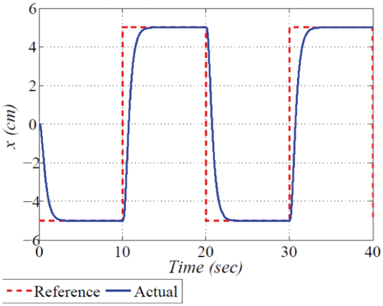
Figure 4: Simulations: ball position

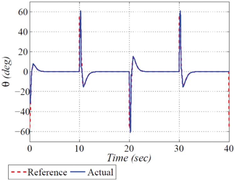
Figure 5: Simulations: beam angle

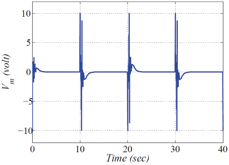
Figure 6: Simulations: controlled voltage

8  Experimental Results

To investigate the real-time performance of balancing the ball on a beam, the IDI control law developed in Section 5 is implemented on Quanser's ball and beam real hardware, as shown in Fig. 7, which proves to be a benchmark testbed for testing and validating control techniques.

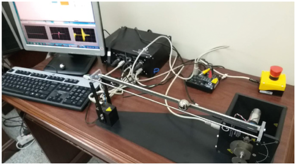
Figure 7: Experimental setup

The experimental setup comprised the power module VoltPAQ-X1 for supplying voltage to the rotary servo motor module. The servo motor is placed at the right corner of the beam to move the beam in an upward and downward direction. The ball placed on the beam rolls on the track accordingly by changing the slope of the beam. The ball position and the angular position feedback commands are sent to the computer through Quanser's Q8-USB data acquisition card. The communication between Simulink/MATLAB and the experimental hardware is accomplished through the QUARC software. The sampling time is chosen to be 2ms for all the experiments.

8.1 Step Response Analysis

In this analysis, the core objective is to present the comparative analysis of IDI control with classical Linear Quadratic Regulator (LQR) and Fractional Order Control (FOC) strategies. The ball is commanded to follow the step input profile in this setup. The initial position of system states are x=−18cm, x˙=0cm, θl=0deg, and θ˙l=0deg, whereas the desired step command is set to be xd=10cm. The three control methodologies were implemented on a practical BBS test bench, and the tracking curves of ball position, beam angle, and the controlled voltages are shown in Figs. 8–10. It is evident from Fig. 8 that the response curves of positional tracking with IDI control are faster in terms of rising time and settling time.

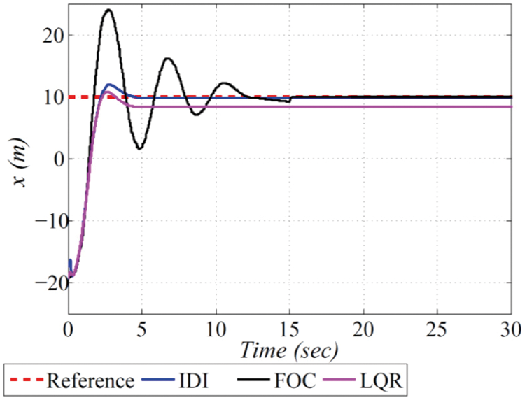
Figure 8: Experimental results: ball position

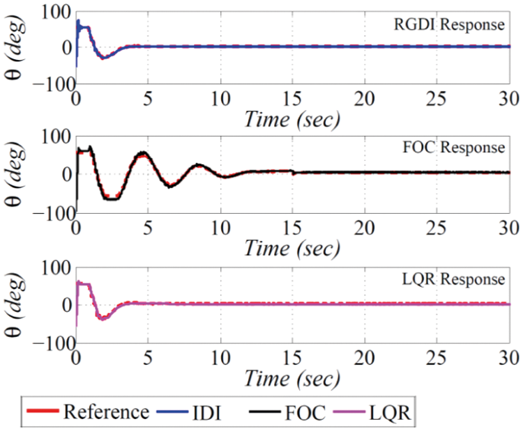
Figure 9: Experimental results: attitude tracking

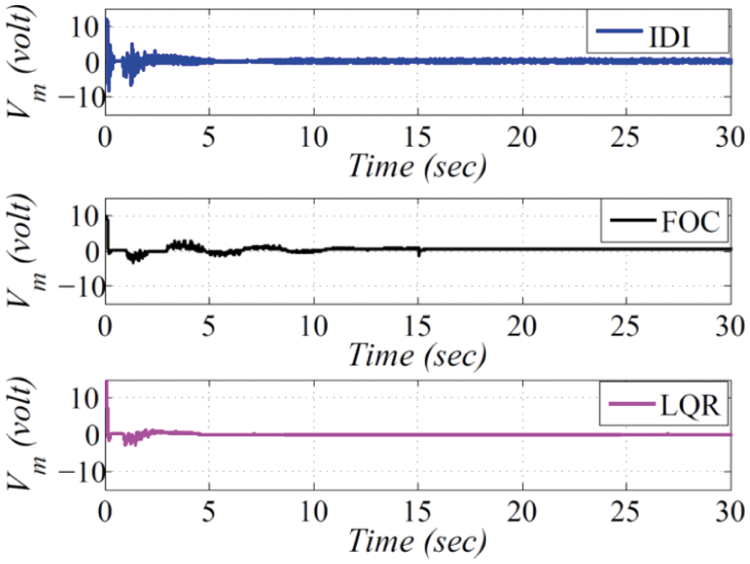
Figure 10: Experimental results: controlled voltage

Furthermore, the FOC suffers from high overshoot, whereas many steady-state errors were observed in the LQR response. On the other hand, the IDI controller demonstrates very stable time-domain performance near reference input with less overshoot and steady-state error. The time evolution of desired and actual angular profiles and the time histories of the controlled voltages generated in response to the step input command are shown in Figs. 9 and 10, respectively.

8.2 Disturbance Rejection Capability

This section highlighted the disturbance rejection capability of the IDI controller when the ball is subjected to some manual disturbances. The ball position on the beam in a steady state is stimulated by tapping the ball at different time instants. The ball position plot under the effect of disturbances is shown in Fig. 11. It is evident that when disturbances are applied, the ball position is perturbed but immediately returns to its stable position by control reaction and re-stabilized. The jerks appeared in the angular profile due to manual perturbations, which are depicted in Fig. 12. The controlled voltage under the supplied capacity is displayed in Fig. 13, whose magnitude fluctuates in response to the applied disturbances. The experimental results demonstrate better disturbance rejection capability and intelligent attributes of IDI control.

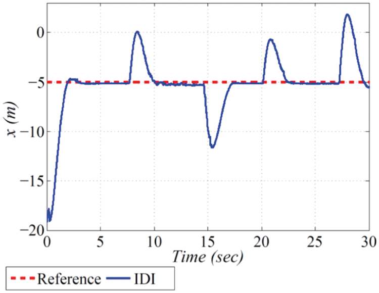
Figure 11: Experimental results: ball position

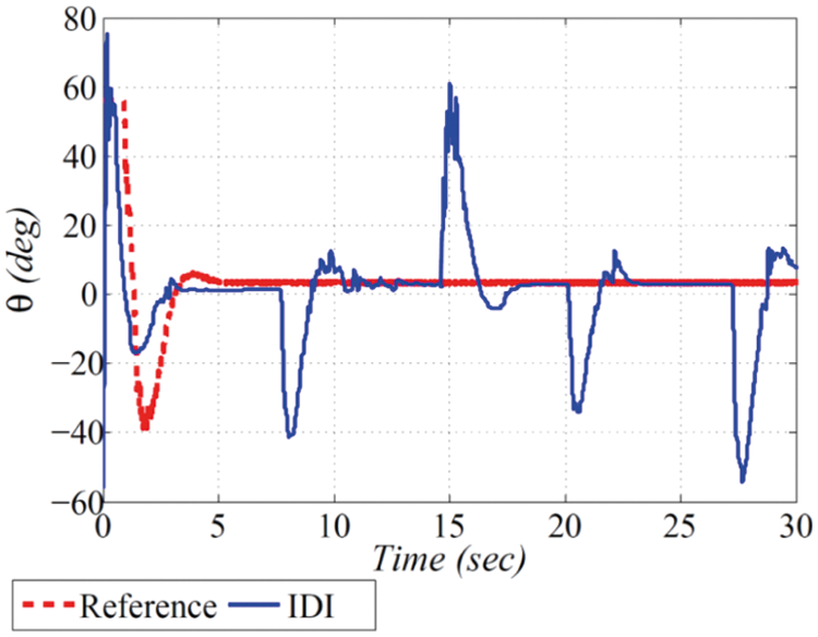
Figure 12: Experimental results: attitude tracking

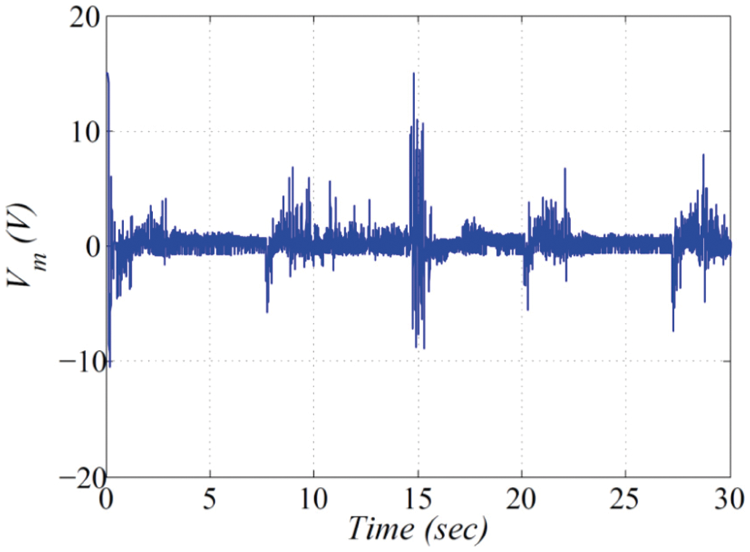
Figure 13: Experimental results: controlled voltage

8.3 Square-wave Tracking

In this plot, the controllers’ capability is further analyzed by commanding a reference square wave profile with an amplitude of ±20m with 0.05Hz frequency and the variation of 20% in the system dynamical parameters. The time evolution of the critical performance indices is illustrated in Figs. 14–16. The smooth tracking response of the ball's position placed on the beam in response to the square wave input command is shown in Fig. 14. The rotary servo angular position tracking curve required to steer the ball to follow the square waveform command and the control effort in the form of generated controlled voltage are shown in Figs. 15 and 16, respectively.

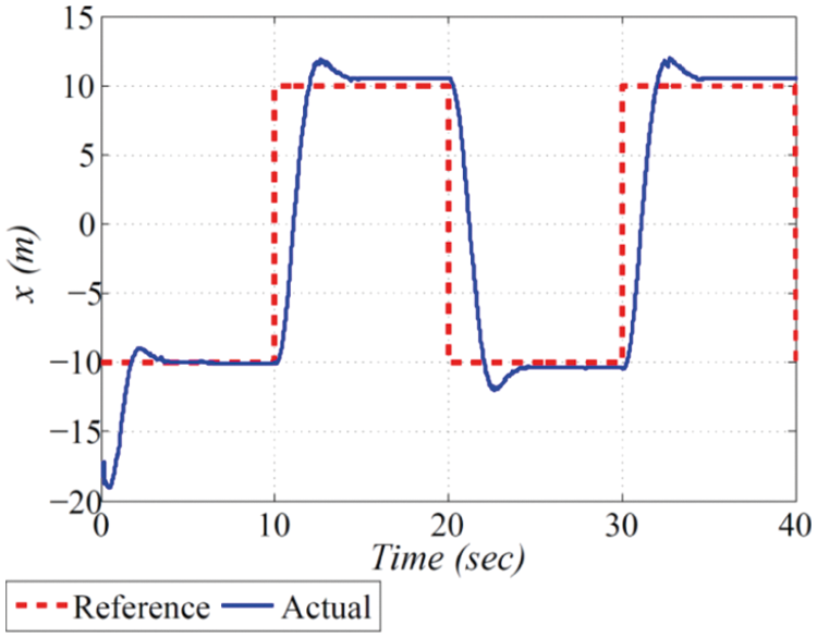
Figure 14: Experimental results: ball position

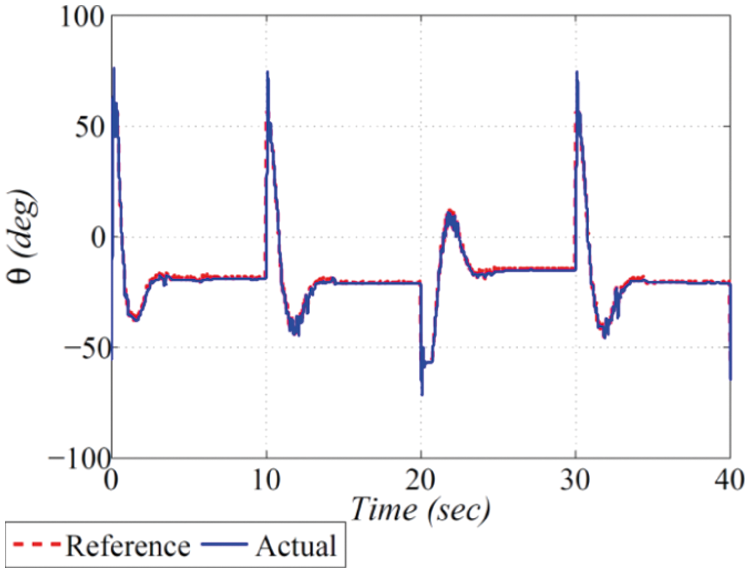
Figure 15: Experimental results: attitude tracking

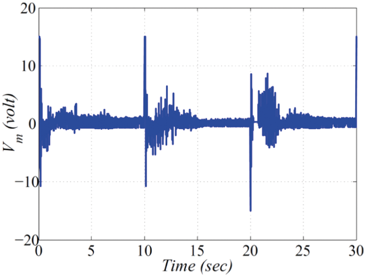
Figure 16: Experimental results: controlled voltage

While examining the different behaviors of the controller response in the simulation and experimental results, it is claimed that the proposed controller proves itself a reasonable control approach for stabilizing the under-actuated electro-mechanical systems.

9  Conclusion

This paper investigates the performance of IDI control for a standard nonlinear ball and beam unstable system. A two-loops structured control is implemented in which PD control is responsible for generating the desired servo angle command based on the positional error of the ball placed on the beam. Furthermore, IDI control is engaged in the inner loop for precise attitude tracking. The results are verified through computer simulations and experimental studies in a MATLAB environment. Furthermore, a comparative analysis is presented, which exhibits the superior performance of IDI control over LQR and FOC in terms of faster error convergence with lesser steady-state error. Hence the proposed methodology is quite appealing and feasible for practical electro-mechanical systems.

Acknowledgement: The authors extend their appreciation to the Deputyship for Research & Innovation, Ministry of Education in Saudi Arabia for funding this research work through the Project Number (IFPRC-023-135-2020) and King Abdulaziz University, DSR, Jeddah, Saudi Arabia.

Funding Statement: This research work was funded by Deputyship for Research & Innovation, Ministry of Education in Saudi Arabia under Grant No. (IFPRC-023-135-2020).

Conflicts of Interest: The authors declare that they have no conflicts of interest to report regarding the present study.

References

 1.  J. Apkarian, P. Karam, M. Levis and H. Gurocak, Quanser Innovative Edutech Laboratory Guide-Ball and Beam Experiment, Canada: Quanser Inc., 2012. [Google Scholar]

 2.  I. M. Mehedi, U. M. Al-Saggaf, R. Mansouri and M. Bettayeb, “Two degrees of freedom fractional controller design: Application to the ball and beam system,” Measurement, vol. 135, pp. 13–22, 2019. [Google Scholar]

 3.  J. Hauser, S. Sastry and P. Kokotovic, “Nonlinear control via approximate input-output linearization: The ball and beam example,” IEEE Transactions on Automatic Control, vol. 37, no. 3, pp. 392–398, 2002. [Google Scholar]

 4.  D. N. Kouya and F. A. Okou, “A new adaptive state feedback controller for the ball and beam system,” in Canadian Conf. on Electrical and Computer Engineering (CCECE), Niagara Falls, Canada, pp. 247–252, 2011. [Google Scholar]

 5.  D. Martinez and F. Ruiz, “Nonlinear model predictive control for a ball and beam,” in 4th Colombian Workshop on Circuits and Systems (CWCAS), Barranquilla, Colombia, pp. 1–5, 2012. [Google Scholar]

 6.  T. Wu and Y. T. Juang, “Adaptive fuzzy sliding-mode controller of uncertain nonlinear systems,” ISA Transactions, vol. 47, no. 3, pp. 279–285, 2008. [Google Scholar]

 7.  A. Nejadfard, M. J. Yazdanpanah and I. Hassanzadeh, “Riction compensation of double inverted pendulum on a cart using locally linear neuro-fuzzy model,” Neural Computing and Applications, vol. 22, no. 2, pp. 337–347, 2013. [Google Scholar]

 8.  W. Luhao and S. Zhanshi, “Lqr-fuzzy control for double inverted pendulum,” in Int. Conf. on Digital Manufacturing & Automation, Changcha, China, pp. 900–903, 2010. [Google Scholar]

 9.  P. Feng, L. Lu and X. Dingyu, “Double inverted pendulum sliding mode variation structure control based on fractional order exponential approach law,” in Proc. CCDC, Guiyang, China, pp. 5077–5080, 2013. [Google Scholar]

10. R. M. Nagarale and B. M. Patre, “Decoupled neural fuzzy sliding mode control of nonlinear systems,” in Proc. FUZZ-IEEE, Hyderabad, India, pp. 1–7, 2013. [Google Scholar]

11. Z. Song and K. Sun, “Adaptive backstepping sliding mode control with fuzzy monitoring strategy for a kind of mechanical system,” ISA Transactions, vol. 53, no. 1, pp. 125–133, 2014. [Google Scholar]

12. M. Mehdi, M. Rehan and F. M. Malik, “A novel anti-windup framework for cascade control systems: An application to underactuated mechanical systems,” ISA Transactions, vol. 3, no. 1, pp. 802–815, 2014. [Google Scholar]

13. I. M. Mehedi, U. M. Al-Saggaf, R. Mansouri and M. Bettayeb, “Stabilization of a double inverted rotary pendulum through fractional order integral control scheme,” International Journal of Advanced Robotic Systems, vol. 16, no. 4, pp. 1–9, 2019. [Google Scholar]

14. I. M. Mehedi, “State feedback based fractional order control scheme for linear servo cart system,” Journal of Vibroengineering, vol. 20, no. 1, pp. 782–792, 2018. [Google Scholar]

15. U. M. Al-Saggaf, I. M. Mehedi, R. Mansouri and M. Bettayeb, “Rotary flexible joint control by fractional order controllers,” International Journal of Control Automation and Systems, vol. 15, no. 6, pp. 2561–2569, 2017. [Google Scholar]

16. U. M. Al-Saggaf, I. M. Mehedi, R. Mansouri and M. Bettayeb, “State feedback with fractional integral control design based on the bode's ideal transfer function,” International Journal of Systems Science, vol. 47, no. 1, pp. 149–161, 2016. [Google Scholar]

17. M. Bettayeb, C. Boussalem and R. Mansouri, “Stabilization of an inverted pendulum-cart system by fractional pi-state feedback,” ISA Transactions, vol. 53, no. 2, pp. 508–516, 2014. [Google Scholar]

18. A. Young, C. Cao and N. Hovakimyan, “Control of a nonaffine double-pendulum system via dynamic inversion and time-scale separation,” in Proc. ACC, Minneapolis, MN, USA, pp. 6–12, 2006. [Google Scholar]

19. A. I. Iskanderani and I. M. Mehedi, “Experimental application of robust and converse dynamic control for rotary flexible joint manipulator system,” Mathematical Problems in Engineering, vol. 2021, Article ID 8917134, pp. 1–9, 2021. [Google Scholar]

20. A. Ben-Israel and T. N. Greville, Generalized Inverses: Theory and Applications, Piscataway, NJ, USA, Springer, 2003. [Google Scholar]

21. I. M. Mehedi, H. S. M. Shah, U. M. Al-Saggaf, R. Mansouri and M. Bettayeb, “Adaptive fuzzy sliding mode control of a pressure-controlled artificial ventilator,” Journal of Healthcare Engineering, vol. 2021, Article ID 1926711, pp. 1–10, 2021. [Google Scholar]

22. I. M. Mehedi, H. S. M. Shah, U. M. Al-Saggaf, R. Mansouri and M. Bettayeb, “Fuzzy PID control for respiratory systems,” Journal of Healthcare Engineering, vol. 2021, Article ID 7118711, pp. 1–6, 2021. [Google Scholar]

23. I. M. Mehedi, U. Ansari and U. M. Al Saggaf UM, “Three degree of freedom rotary double inverted pendulum stabilization by using robust generalized dynamic inversion control: Design and experiments,” Journal of Vibration and Control, vol. 26, no. 23–24, pp. 2174–2184, 2020. [Google Scholar]

24. I. M. Mehedi, U. M. Al-Saggaf and S. S. Ali, “Design and simulation of fractional order control scheme for rotary flexible link,” in Proc. ICIAS, Kuala Lumpur, Malaysia, pp. 1–5, 2018. [Google Scholar]

25. I. M. Mehedi, “Full state-feedback solution for a flywheel based satellite energy and attitude control scheme,” Journal of Vibroengineering, vol. 19, no. 5, pp. 3522–3532, 2017. [Google Scholar]

26. J. Apkarian, M. Levis and H. Gurocak, Quanser Innovative Edutech-Laboratory Guide-SRV02 Laboratory User Manual, Canada: Quanser Inc, 2009. [Google Scholar]

27. H. Khalil, Nonlinear Systems, NJ, USA, Pearson: Prentice-Hall, 1996. [Google Scholar]

This work is licensed under a Creative Commons Attribution 4.0 International License, which permits unrestricted use, distribution, and reproduction in any medium, provided the original work is properly cited.