Computers, Materials & Continua DOI:10.32604/cmc.2022.023057
Article

A Post-Processing Algorithm for Boosting Contrast of MRI Images

B. Priestly Shan1, O. Jeba Shiney1, Sharzeel Saleem2, V. Rajinikanth3, Atef Zaguia4 and Dilbag Singh5,*

1Department of Electronics & Communication Engineering, Chandigarh University, Mohali, 140413, India
2Department of Electrical, Electronics & Communication Engineering, Galgotias University, Greater Noida, 201310, India
3Department of Electronics and Instrumentation Engineering, St. Joseph's College of Engineering, Chennai, 600119, Tamil Nadu, India
4Department of Computer Science, College of Computers and Information Technology, Taif University, Taif, 21944, Saudi Arabia
5School of Electrical Engineering and Computer Science, Gwangju Institute of Science and Technology, Gwangju, 61005, Korea
*Corresponding Author: Dilbag Singh. Email: dggill2@gmail.com
Received: 26 August 2021; Accepted: 16 November 2021

Abstract: Low contrast of Magnetic Resonance (MR) images limits the visibility of subtle structures and adversely affects the outcome of both subjective and automated diagnosis. State-of-the-art contrast boosting techniques intolerably alter inherent features of MR images. Drastic changes in brightness features, induced by post-processing are not appreciated in medical imaging as the grey level values have certain diagnostic meanings. To overcome these issues this paper proposes an algorithm that enhance the contrast of MR images while preserving the underlying features as well. This method termed as Power-law and Logarithmic Modification-based Histogram Equalization (PLMHE) partitions the histogram of the image into two sub histograms after a power-law transformation and a log compression. After a modification intended for improving the dispersion of the sub-histograms and subsequent normalization, cumulative histograms are computed. Enhanced grey level values are computed from the resultant cumulative histograms. The performance of the PLMHE algorithm is compared with traditional histogram equalization based algorithms and it has been observed from the results that PLMHE can boost the image contrast without causing dynamic range compression, a significant change in mean brightness, and contrast-overshoot.

Keywords: Contrast enhancement; histogram equalisation; image quality; magnetic resonance imaging; medical image analysis; post-processing

1  Background & Problem Domain

Magnetic Resonance Imaging (MRI) is a medical imaging modality used to visualize the internal organs of the human body. The MRI is widely used for the diagnosis of a broad spectrum of diseases like ischemic stroke [1], Autism Spectrum Disorder (ASD) [2], Parkinson's disease [3], brain tumors [4], Schizophrenia [5], intracranial Tuberculosis [6], pancreatic cancer [7], Osteo Arthritis [8], prostate cancer [9] and Endometriosis [10]. Because of hardware limitations, images obtained from low-field MRI scanners are of low resolution, low acutance, and low contrast. The presence of noise is another factor that reduces the quality of MR images. Hence, post-processing algorithms are extensively used in medical imaging to improve the quality of MR images.

The post-processing algorithms used for improving the quality of MR images include bias correction [11,12], denoising/smoothing filters [13,14], super-resolution techniques [15,16], sharpening schemes [17], and contrast enhancement. The contrast enhancement improves the visibility of subtle changes and fine structures in the MR images. Contrast boosting is helpful to make the interpretation of MR images easier and the diagnosis more accurate. Segmentation of brain structures or anomalies is a usual procedure involved in the automated analysis of MRI. For example, segmentation of the hippocampus is a step involved in the automated diagnosis of Alzheimer's Disease (AD) from MRI [18]. Similarly, accurate segmentation of brain tumors is an important step in MRI-guided automated surgery and radiation treatment planning [19]. Contrast boosting is helpful to improve the efficiency of segmentation algorithms.

2  Related Work

Among the contrast boosting algorithms, Histogram Equalization (HE) is the one that is widely used on medical images. However, HE has several limitations. HE causes over-enhancement and amplifies noise. It intolerably changes the mean brightness of the image. Several algorithmic modifications of HE meant for incorporating brightness-preserving characteristics are available in the literature. Based on the application, the modifications of HE can be categorized in different ways. Certain modifications of HE are exclusively intended for enhancing color images. The image enhancement algorithm based on the combination of reflectance guided HE and ‘comparametric approximation’ proposed by Wu et al. [20] is a typical example of this. Another example is the white balancing algorithm proposed by Kumar et al. [21]. Certain other modifications of HE are exclusively meant for enhancing the contextual information rather than the region-wise contrast. The Fuzzy-Contextual Contrast Enhancement (FCCE) scheme proposed by Parihar et al. [22] is an example of this. In the FCCE, the enhanced image is computed from the histogram of fuzzy-based local contrast, rather than the intensity histogram.

Apart from algorithms for color image enhancement and improving the local contrast (contextual information), techniques suitable for enhancing the global contrast of greyscale images are also available in the literature. The Adaptive Histogram Equalization (AHE) [23], Non-parametric Modified Histogram Equalization (NMHE) [24], Plateau Limit-based Tri-histogram Equalization (PLTE) [25], Triple Clipped Dynamic Histogram Equalization based on Standard Deviation (TCDHE-SD) [26], Clipped and Thresholded Weighted Histogram Equalization (CTWHE) [27] and Contrast Limited Adaptive Histogram Equalization (CLAHE) [28,29] are certain examples suitable for boosting global contrast of greyscale images.

In the AHE, the normalized histogram is clipped with respect to its mean amplitude, and the cumulative histogram computed from the clipped histogram is normalized to a range 0–1, if the ratio of maximum amplitude and mean amplitude of the normalized histogram is greater than an arbitrary value (suggested as 10). If the ratio of maximum amplitude and mean amplitude of the histogram is less than the arbitrary value, clipping and normalization steps are waived. Following this, the cumulative histogram is subjected to an exponential weighting. In the weighting process, the ratio of the total sum of values in the cumulative histogram and the highest possible intensity value is used as the exponent.

In NMHE, to avoid amplification of noise, only the pixels which exhibit a relatively higher value of gradient with respect to their neighbors are considered while computing the histogram. The histogram normalized to the range [0 1] is clipped with respect to a threshold value equal to the reciprocal of the maximum possible number of grey levels (256 in a unit8 image). A linear combination of the clipped histogram and a uniform histogram is computed following this. The amplitude of the uniform histogram is equal to the reciprocal of the maximum possible number of grey levels, at all grey levels. In the linear combination, the total sum of the differences between corresponding values in the uniform histogram and the clipped histogram is used as the weight of the clipped histogram. The difference of the total sum of the differences between corresponding values in the uniform histogram and the clipped histogram and one is used as the weight of the uniform histogram, in the linear combination. A cumulative histogram computed from the output histogram of the linear combination and the enhanced image is computed from the cumulative histogram. To compensate the change in mean brightness, the output of the histogram equalization is subjected to a gamma transformation. The ratio of the log of the normalized value of the mean brightness of the input image and the log of the normalized value of the mean brightness of the output of histogram equalization is used as the value of gamma.

In PLTE, the histogram is clipped with respect to the average of mean and median f amplitude values in it. The clipped histogram is partitioned into three sub-histograms with respect to two threshold values. The first threshold is the sum of the minimum intensity of the input image and the standard deviation of the pixel intensities in it. The second threshold is the difference between the highest intensity of the input image and the standard deviation of the pixel intensities in it. Each sub-histogram is equalized individually.

In the TCDHE-SD, the histogram is partitioned into three sub-histograms with respect to two threshold values. The first threshold is the difference between the mean intensity of the input image and the product of 0.43 and the standard deviation of the pixel intensities in it. The second threshold is the sum of the mean intensity of the input image and the product of 0.43 and the standard deviation of the pixel intensities in it. Each sub-histogram is clipped. The clip-limit used for the first sub-histogram is the product of the sum of values in the first sub-histogram and the reciprocal of the difference between the first threshold and minimum intensity of the input image. The clip-limit used for the second sub-histogram is the product of the sum of values in the second sub-histogram and the reciprocal of the difference between the second threshold and first threshold. The clip-limit used for the third sub-histogram is the product of the sum of values in the third sub-histogram and the reciprocal of the difference between the second threshold and maximum intensity of the input image. A cumulative histogram is computed from each clipped sub-histogram after normalizing with the total sum of values in it. Enhanced grey level values are computed from the cumulative histograms.

In CTWHE, the histogram is clipped first with respect to an arbitrary clip-limit. The histogram amplitudes below another arbitrarily chosen threshold value are made 0. The clipped and thresholded histogram is subjected to a Power-Law Transformation. The cumulative histogram is computed from the weighted histogram. Enhanced grey levels are computed from the cumulative histogram.

In the CLAHE, the input image is first partitioned into non-overlapping blocks. The histograms of the individual blocks are clipped against a user-defined clip-limit. The remaining pixels resulting from the clipping process are filled back to the histogram bins. The cumulative histogram is computed after the refilling process. The cumulative histogram is subjected to a modification based on a user-defined histogram specification. Three types of histogram specifications are mostly used in CLAHE. These specifications are uniform, exponential, Rayleigh. The block-wise enhancement procedure followed in CLAHE results in artificial edges among the blocks. To reduce the impact of this drawback pixel values at the boundary of the blocks are calculated with the help of a bilinear interpolation algorithm.

3  Limitations of Existing Techniques & Motivation

In the reflectance-guided HE, estimation of the reflectance component is based on the Retinex theory. Retinex theory is applicable for image formation in a digital camera and it does not account for the image reconstruction process in MRI. In the white balancing algorithm, information from all color channels is used simultaneously. Hence, white balancing is not suitable for greyscale images like MRI. Methods like FCCE can make the image sharper. FCCE does not increase the grey level contrast between objects and regions lying spatially apart.

The AHE, NMHE, PLTE, TCDHE-SD, and CTWHE do not have brightness-preserving characteristics. The NMHE, PLTE, TCDHE-SD and CTWHE compress the dynamic range of the image. The output images produced by any ideal contrast boosting technique should occupy the full dynamic range. Drastic changes in brightness features, induced by post-processing are not appreciated in medical imaging as the grey level values have certain diagnostic meanings. CLAHE has some other serious limitations also. The bilinear interpolation used to compute the grey levels along the borders of the blocks does not suppress the inter-block edges caused by the block-wise equalization. The quality of the enhanced images obtained from CLAHE heavily depends on the choice of multiple user-defined parameters such as clip-limit, size of the tile, targeted histogram shape, and model parameters of targeted histogram specification. The process of adjusting many such user-defined parameters simultaneously is very complex. Hence CLAHE is less user-friendly. As a solution to these problems, a post-processing algorithm termed as Power-law and Logarithmic Modification-based Histogram Equalization (PLMHE) that has excellent feature-preserving features, for boosting the contrast of MR images is proposed in this paper.

4  Power-law and Logarithmic Modification-based Histogram Equalization (PLMHE)

The first step in the PLMHE is the computation of the histogram of the input image. Let the histogram of the input image ‘X’ be:

Hk,k=0,1,2,……L−1andk∈X(1)

In Eq. (1), ‘Hk’ represents the number of occurrences of an arbitrary grey level, ‘k’ in the input image, ‘X’ and ‘L−1’ is the maximum possible grey level value. In an image with bit-depth equal to 8 (uint8 image), the maximum possible grey level value is, L−1=28−1=255.

In the second step, the histogram, ‘Hk’ is subjected to an adaptive power-law transformation as:

Pk=(Hk)γ,γ=eα&α=1(L−1)(∑k=0L−1⁡kHk/∑k=0L−1⁡Hk)(2)

In Eq. (2), ‘α’ is normalised value of the mean intensity of the input image, ‘X’. The power-law transformation is referred to as ‘adaptive’ because the exponent, ‘γ’ is determined adaptively from the normalised value of the mean intensity of the input image. The normalized value of the mean intensity of the input image can be computed alternatively as:

α=1RC∑r=1R⁡∑c=1C⁡(X(r,c)/(L−1))(3)

In Eq. (3), ‘R’ and ‘C’ respectively are the number of rows and number of columns in the input image. From Eqs. (2) and (3), it can be inferred that the range of ‘α’ is [0 1]. This implies,

limα→0⁡eα=1&limα→1⁡eα≈2.72(4)

From Eqs. (2) and (4), it can be understood that the higher is the normalized value of the mean intensity, the histogram undergoes a higher level of amplification. A log transformation is applied to the histogram obtained after the power-law transformation, to avoid over-enhancement and saturation. The log transformation is,

Qk=β(log⁡(1+Pk)(5)

In Eq. (5), ‘β’, is a user-defined parameter within a range, 0≤β≤1, which further penalises the histogram for restricting the over-enhancement and saturation. Preservation of mean brightness is a major concern in histogram equalization-based contrast boosting. Hence, for preserving the mean brightness, the principle of bi-histogram equalization [30] is adopted. The histogram obtained after the log transformation ‘Qk’ is split into two sub-histograms, with respect to an adaptive intensity threshold, ‘τ’. The first sub-histogram obtained from the histogram partitioning is,

Ak=Qk,k=0,1,2……τ(6)

The second sub-histogram is,

Bk=Qk,k=τ+1,τ+2,τ+3……(L−1)(7)

The arbitrary threshold ‘τ. ’ in Eqs. (6) and (7) is the product of the total number of possible grey levels, ‘L’ and the normalized value of the mean intensity of the input image, ‘α’, such that, τ=Lα. The standard deviations of each sub-histograms are added to them to enhance their dispersion. Improving the dispersion of the histograms is helpful to ensure better contrast gain. The modified sub-histograms after adding the respective values of standard deviation are,

Dk=Ak+σA,σA=(1τ+1∑k=0τ⁡(Ak−μA)2)1/1 22(8)

Ek=Bk+σB,σB=(1(L−τ+1)∑k=τ+1L−1⁡(Bk−μB)2)1/1 22(9)

In Eqs. (8) and (9), ‘σA’ and ‘σB’ respectively are standard deviations of amplitude values in the sub-histograms ‘Ak’ and ‘Bk’. The notions, ‘μA’ and ‘μB’ respectively denote the mean amplitudes of the sub-histograms ‘Ak’ and ‘Bk’ given by,

μA=1τ+1∑k=0τ⁡Ak&μB=1(L−τ+1)∑k=τ+1L−1⁡Bk(10)

The modified sub-histograms, ‘Dk’ and ‘Ek’ are normalized as,

Fk=Dk/∑k=0τ⁡Dk&Gk=Ek/∑k=τ+1L−1⁡Ek(11)

The histogram at various levels of processing described in Eqs. (1) to (11) is shown in Fig. 1. Relatively high amplitudes the original histogram (Fig. 1a) is amplified to a greater degree by the PLT as apparent in Fig. 1b. Readers should note that the multiplier corresponding to the Y-axis in Fig. 1b is 105. The nonlinear log transform compresses the histogram amplitudes as seen in Fig. 1c. Uniformly adding the respective values of the standard deviation to the sub-histograms, emphasize the low amplitude values and penalizes high amplitude values, upon normalization as evident in Figs. 1c–1i.

Figure 1: Histogram at various levels of processing (a) Original histogram (b) After power-law transform (c) After log transform (d) First sub-histogram (e) Second sub-histogram (f) First sub-histogram after modification (g) Second sub-histogram after modification (h) modified first sub-histogram after normalization (h) modified second sub-histogram after normalization

The enhanced grey level, ‘i’ corresponding to the original grey level, ‘k’ is

i={((τ−Xmin)∑j=0k⁡Fj)+Xminifk≤τ((Xmax−(τ+1))∑j=τ+1k⁡Gj)+(τ+1)ifk>τ(12)

In Eq. (12), ‘Xmin’ and ‘Xmax’ respectively are the minimum and maximum values of grey levels present in the input image, ‘X’. Each intensity, ‘k’ in the input image, ‘X’ is replaced by the corresponding enhanced intensity, ‘i’ to obtain the contrast-boosted image.

The steps involved in PLMHE described above are pictorially depicted in Fig. 2. The histogram of the input image is subjected to a PLT and a log compression. The resultant histogram is partitioned into two sub-histograms with respect to an intensity threshold. The value of the exponent in the PLT is an exponential function of normalized mean intensity of the input image. The intensity threshold is the product of normalized mean intensity of the input image and the maximum possible number of grey levels. Each sub-histogram is modified by adding the standard deviation of values in it for enhancing the dispersion. After normalizing the modified sub-histograms with the total sum of values in them, cumulative histograms are computed. Enhanced grey level values are computed from the cumulative histograms.

Figure 2: Schematic of the steps involved in PLMHE

5  Test Images & System Requirements

A data set comprising 100 MR slices are used in this experiment. It is a well-established dataset already used in literature for evaluating the performance of image enhancement algorithms [31–33]. Images in the data set are acquired with the help of a 1.5 Tesla 2D MRI scanner manufactured by GE Medical Systems (Model: Signa HDxt), available at Hind Labs, Government Medical College Kottayam, Kerala, India. The Series of acquisitions is MR Spectroscopy. Slice thickness and inter-slice gap set during the image acquisition are 5 and 1.5 mm, respectively. Images from T1 Fast Spin-Echo Contrast-Enhanced (FS-ECE), T2 Fluid Attenuation Inversion Recovery (FLAIR), Diffusion-Weighted Imaging (DWI), Gradient Recalled Echo (GRE) and 1000b Array Spatial Sensitivity Encoding Technique (ASSET) pulse sequences are used. Proposed and state-of-the-art enhancement algorithms are simulated using Matlab® 2020a. The software is installed on a desktop computer operating on Windows 7 with 8 GB RAM. The system runs on an i3–2100 processor with 2 cores and a maximum speed of 3.1 GHz.

6  Results & Discussions

In this section, the performance of PLMHE is tested against its alternatives, namely, AHE, NMHE, PLTE, TCDHE-SD, CTWHE and CLAHE, via subjective inspection of their output images and with the help of objective quality metrics like Patch-based Contrast Quality Index (PCQI) [34], Absolute Mean Brightness Error (AMBE) [35], Over-Contrast Measure (OCM) [36] and Dynamic Range (DR).

6.1 Subjective Evaluation

Output images of AHE, NMHE, PLTE, TCDHE-SD, CTWHE, CLAHE, and PLMHE on three test images are furnished in Figs. 3–5. Output images of AHE (Figs. 3b, 4b and 5b) and NMHE (Figs. 3c, 4c, and 5c) are significantly brighter than the input images. Rather than increasing the brightness, the grey level difference between different structures has not improved. However, the increase in brightness is not as severe in NMHE as AHE. Output images of PLTE (Figs. 3d, 4d and 5d), TCDHE-SD (Figs. 3e, 4e and 5e), and CTWHE (Figs. 3f, 4f and 5f), appear to be unnatural. Inherent brightness features of the input images are not maintained during the contrast boosting. Drastically amplified background noise is visible in the output images of CTWHE. Being a local enhancement scheme, CLAHE sharpens the texture instead of improving global contrast among the structures as visible in Figs. 3g, 4g and 5g. PLMHE ((Figs. 3h, 4h and 5h)), improves the global contrast among the structures by maintaining inherent brightness features of the input images. The issues of noise amplification observed in TCDHE-SD and textural sharpening noted in CLAHE, are absent in PLMHE. On all 100 test images, the PLMHE is found to be better than AHE, NMHE, PLTE, TCDHE-SD, CTWHE, and CLAHE.

Figure 3: Output of various contrast boosting schemes (a) Input image 1 (b) AHE (c) NMHE (d) PLTE (e) TCDHE-SD (f) CTWHE (g) CLAHE (h) PLMHE

6.2 Objective Evaluation

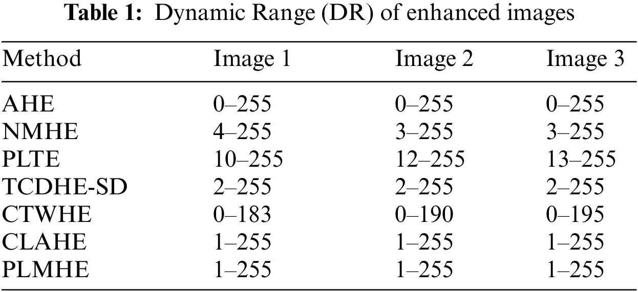
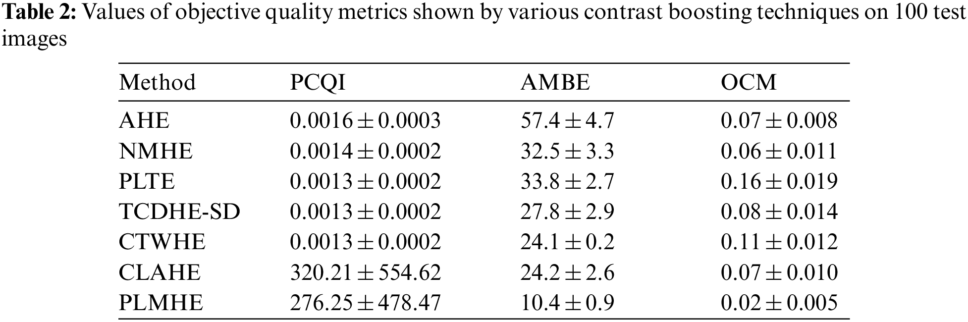
Any ideal contrast boosting algorithm should maximize the image contrast without causing dynamic range compression, a significant change in mean brightness, and over-enhancement/contrast-overshoot. These aspects are considered in this paper for objectively evaluating the quality of enhanced images. The first objective measure, Dynamic Range (DR) reflects the dynamic range compression. Ideally, grey levels in an enhanced image should occupy the full dynamic range. The ideal value of DR is 0–255, in a uint8 image. Another quality metric, the Patch-based Contrast Quality Index (PCQI) is used to measure the grey level contrast of enhanced images. Absolute Mean Brightness Error (AMBE) is employed to quantify the shift in mean brightness. Over-Contrast Measure (OCM) indicates the degree of contrast-overshoot. The OCM is a bounded statistic with a range [0 1]. The value of PCQI should be as high as possible. The values of the AMBE and OCM are expected to be as low as possible.

Figure. 4: Output of various contrast boosting schemes (a) Input image 2 (b) AHE (c) NMHE (d) PLTE (e) TCDHE-SD (f) CTWHE (g) CLAHE (h) PLMHE

Values of DR of enhanced images from various contrast boosting techniques on three test images are shown in Tab. 1. From Tab. 1 it is evident that NMHE, PLTE, TCDHE-SD, and CTWHE compress the dynamic range of the image. The issue of dynamic range compression is more severe in PLTE and CTWHE compared to NMHE and TCDHE-SD. AHE, CLAHE, and PLMHE are free from the above issue. Outputs of all three algorithms cover almost the full dynamic range in a relatively better way.

Values of objective quality metrics shown by various contrast boosting techniques on 100 test images are shown in Tab. 2. Very high values of PCQI in Tab. 2, exhibited by CLAHE and PLMHE indicate that they can produce output images with very high perceptual contrast. Compared to the AHE, NMHE, PLTE, TCDHE-SD, CTWHE, and CLAHE, PLMHE exhibits the lowest values of AMBE and OCM. The lowest value of AMBE shown by PLMHE reflects its excellent ability to preserve brightness features. The lowest value of OCM shown by PLMHE confirms that it is free from the issue of contrast-overshoot. Even though CLAHE has exhibited high values of PCQI, it shows AMBE and OCM values significantly higher than that of the PLMHE. CLAHE is prone to contrast-overshoot, and it is inferior to PLMHE in terms of brightness-preserving features.

Figure 5: Output of various contrast boosting schemes (a) Input image 3 (b) AHE (c) NMHE (d) PLTE (e) TCDHE-SD (f) CTWHE (g) CLAHE (h) PLMHE

7  Conclusion and Future Scope

A post-processing algorithm termed as Power-law and Logarithmic Modification-based Histogram Equalization (PLMHE) that has excellent feature-preserving features, for boosting the contrast of MR images was proposed in this paper. PLMHE exhibited higher values of PCQI and lower values of AMBE and OCM compared to state-of-the-art contrast boosting algorithms, namely, AHE, NMHE, PLTE, TCDHE-SD, CTWHE, and CLAHE. It was found that outputs images of PLMHE cover the full dynamic range. It has been observed that PLMHE could boost the image contrast without causing dynamic range compression, a significant change in mean brightness, and contrast-overshoot.

The performance of PLMHE was tested in this paper via subjective inspection of the output images and with the help of objective quality metrics like PCQI, AMBE, and OCM. The impact of contrast boosting needs to be further studied on context-specific clinical applications. One constraint encountered during the performance evaluation of PLMHE was lack of a unique objective quality metric that can reflect the overall quality of the enhanced images in terms of perceptual contrast, dynamic range, brightness-preservation, and contrast overshoot. Such a metric can make the performance evaluation of contrast boosting techniques easier and more reliable. The feasibility of PLMHE for hardware implementation needs to be evaluated further on a suitable hardware platform like Field Programmable Gate Array (FPGA).

Acknowledgement: This work was supported by Taif university Researchers Supporting Project Number (TURSP-2020/114), Taif University, Taif, Saudi Arabia.

Funding Statement: This work was supported by Taif university Researchers Supporting Project Number (TURSP-2020/114), Taif University, Taif, Saudi Arabia.

Conflicts of Interest: The authors declare that they have no conflicts of interest to report regarding the present study.

References

 1.  K. C. Ho, W. Speier, H. Zhang, F. Scalzo, S. El-Saden et al., “A machine learning approach for classifying ischemic stroke onset time from imaging,” IEEE Transactions on Medical Imaging, vol. 38, no. 7, pp. 1666–1676, 2019. [Google Scholar]

 2.  J. Wang, L. Zhang, Q. Wang, L. Chen, J. Shi et al., “Multi-class ASD classification based on functional connectivity and functional correlation tensor via multi-source domain adaptation and multi-view sparse representation,” IEEE Transactions on Medical Imaging, vol. 39, no. 10, pp. 3137–3147, 2020. [Google Scholar]

 3.  M. Kim, J. H. Won, J. Youn and H. Park, “Joint-connectivity-based sparse canonical correlation analysis of imaging genetics for detecting biomarkers of Parkinson's disease,” IEEE Transactions on Medical Imaging, vol. 39, no. 1, pp. 23–34, 2020. [Google Scholar]

 4.  Y. Kurmi and V. Chaurasia, “Classification of magnetic resonance images for brain tumour detection,” IET Image Processing, vol. 14, no. 12, pp. 2808–2818, 2020. [Google Scholar]

 5.  Y. Zheng, H. Tong, T. Zhao, X. Guo, H. Xu et al., “Support vector machine classification combined with multimodal magnetic resonance imaging in detection of patients with schizophrenia,” IET Image Processing, vol. 14, no. 11, pp. 2610–2615, 2020. [Google Scholar]

 6.  Y. Cao, J. Mao, H. Yu, Q. Zhang, H. Wang et al., “A novel hybrid active contour model for intracranial tuberculosis MRI segmentation applications,” IEEE Access, vol. 8, pp. 149569–149585, 2020. [Google Scholar]

 7.  Y. Zhang, S. Wang, S. Qu and H. Zhang, “Support vector machine combined with magnetic resonance imaging for accurate diagnosis of paediatric pancreatic cancer,” IET Image Processing, vol. 14, no. 7, pp. 1233–1239, 2020. [Google Scholar]

 8.  I. Iqbal, G. Shahzad, N. Rafiq, G. Mustafa and J. Ma, “Deep learning-based automated detection of human knee joint's synovial fluid from magnetic resonance images with transfer learning,” IET Image Processing, vol. 14, no. 10, pp. 1990–1998, 2020. [Google Scholar]

 9.  H. Jia, Y. Xia, Y. Song, D. Zhang, H. Huang et al., “3D APA-Net: 3D adversarial pyramid anisotropic convolutional network for prostate segmentation in MR images,” IEEE Transactions on Medical Imaging, vol. 39, no. 2, pp. 447–457, 2020. [Google Scholar]

10. O. E. Mansouri, F. Vidal, A. Basarab, P. Payoux, D. Kouamé et al., “Fusion of magnetic resonance and ultrasound images for endometriosis detection,” IEEE Transactions on Image Processing, vol. 29, pp. 5324–5335, 2020. [Google Scholar]

11. Z. Liu, X. Bai, H. Liu and Y. Zhang, “Multiple-surface-approximation-based fcm with interval memberships for bias correction and segmentation of brain MRI,” IEEE Transactions on Fuzzy Systems, vol. 28, no. 9, pp. 2093–2106, 2020. [Google Scholar]

12. P. K. Mishro, S. Agrawal, R. Panda and A. Abraham, “Novel fuzzy clustering-based bias field correction technique for brain magnetic resonance images,” IET Image Processing, vol. 14, no. 9, pp. 1929–1936, 2020. [Google Scholar]

13. G. Chen, B. Dong, Y. Zhang, W. Lin, D. Shen et al., “Denoising of diffusion MRI data via graph framelet matching in x-q space,” IEEE Transactions on Medical Imaging, vol. 38, no. 12, pp. 2838–2848, 2019. [Google Scholar]

14. X. Qiu, Z. Chen, S. Adnan and H. He, “Improved MR image denoising via low-rank approximation and Laplacian-of-Gaussian edge detector,” IET Image Processing, vol. 14, no. 12, pp. 2791–2798, 2020. [Google Scholar]

15. Q. Lyu, H. Shan, C. Steber, C. Helis, C. Whitlow et al., “Multi-contrast super-resolution MRI through a progressive network,” IEEE Transactions on Medical Imaging, vol. 39, no. 9, pp. 2738–2749, 2020. [Google Scholar]

16. Q. Lyu, H. Shan and G. Wang, “MRI Super-resolution with ensemble learning and complementary priors,” IEEE Transactions on Computational Imaging, vol. 6, pp. 615–624, 2020. [Google Scholar]

17. J. Joseph and R. Periyasamy, “Nonlinear sharpening of MR images using a locally adaptive sharpness gain and a noise reduction parameter,” Pattern Analysis and Applications, vol. 22, pp. 273–283, 2019. [Google Scholar]

18. J. H. Morra, Z. Tu, L. G. Apostolova, A. E. Green, A. W. Toga et al., “Comparison of AdaBoost and support vector machines for detecting Alzheimer's disease through automated hippocampal segmentation,” IEEE Transactions on Medical Imaging, vol. 29, no. 1, pp. 30–43, 2010. [Google Scholar]

19. A. Mano and S. Anand, “Method of multi-region tumour segmentation in brain MRI images using grid-based segmentation and weighted bee swarm optimisation,” IET Image Processing, vol. 14, no. 12, pp. 2901–2910, 2020. [Google Scholar]

20. X. Wu, T. Kawanishi and K. Kashino, “Reflectance-guided histogram equalization and comparametric approximation,” IEEE Transactions on Circuits and Systems for Video Technology, vol. 31, no. 3, pp. 863–876, 2021. [Google Scholar]

21. M. Kumar and A. K. Bhandari, “Contrast enhancement using novel white balancing parameter optimization for perceptually invisible images,” IEEE Transactions on Image Processing, vol. 29, pp. 7525–7536, 2020. [Google Scholar]

22. A. S. Parihar, O. P. Verma and C. Khanna, “Fuzzy-contextual contrast enhancement,” IEEE Transactions on Image Processing, vol. 26, no. 4, pp. 1810–1819, 2017. [Google Scholar]

23. S. Kansal and R. K. Tripathi, “New adaptive histogram equalisation heuristic approach for contrast enhancement,” IET Image Processing, vol. 14, no. 6, pp. 1110–1119, 2020. [Google Scholar]

24. S. Poddar, S. Tewary, D. Sharma, V. Karar, A. Ghosh et al., “Non-parametric modified histogram equalisation for contrast enhancement,” IET Image Processing, vol. 7, no. 7, pp. 641–652, 2013. [Google Scholar]

25. A. Paul, P. Bhattacharya, S. P. Maity and B. K. Bhattacharyya, “Plateau limit-based tri-histogram equalisation for image enhancement,” IET Image Processing, vol. 12, no. 9, pp. 1617–1625, 2018. [Google Scholar]

26. M. Zarie, A. Pourmohammad and H. Hajghassem, “Image contrast enhancement using triple clipped dynamic histogram equalisation based on standard deviation,” IET Image Processing, vol. 13, no. 7, pp. 1081–1089, 2019. [Google Scholar]

27. A. K. Bhandari, S. Maurya and A. K. Meena, “MFO-Based thresholded and weighted histogram scheme for brightness preserving image enhancement,” IET Image Processing, vol. 13, no. 6, pp. 896–909, 2019. [Google Scholar]

28. Z. Shi, Y. Feng, M. Zhao, E. Zhang and L. He, “Normalised gamma transformation-based contrast-limited adaptive histogram equalisation with colour correction for sand–dust image enhancement,” IET Image Processing, vol. 14, no. 4, pp. 747–756, 2020. [Google Scholar]

29. H. Lidong, Z. Wei, W. Jun and S. Zebin, “Combination of contrast limited adaptive histogram equalisation and discrete wavelet transform for image enhancement,” IET Image Processing, vol. 9, no. 10, pp. 908–915, 2015. [Google Scholar]

30. Y. T. Kim, “Contrast enhancement using brightness preserving bi-histogram equalization,” IEEE Transactions on Consumer Electronics, vol. 43, no. 1, pp. 1–8, 1997. [Google Scholar]

31. V. R. Simi, D. R. Edla, J. Joseph and V. Kuppili, “Parameter-free fuzzy histogram equalisation with illumination preserving characteristics dedicated for contrast enhancement of magnetic resonance images,” Applied Soft Computing, vol. 93, p. 106364, 2020. https://doi.org/10.1016/j.asoc.2020.106364. [Google Scholar]

32. J. Joseph and R. Periyasamy, “A fully customized enhancement scheme for controlling brightness error and contrast in magnetic resonance images,” Biomedical Signal Processing and Control, vol. 39, pp. 271–283, 2018. [Google Scholar]

33. V. R. Simi, D. R. Edla, J. Joseph and V. Kuppili, “Analysis of controversies in the formulation and evaluation of restoration algorithms for MR images,” Expert Systems with Applications, vol. 135, pp. 39–59, 2019. [Google Scholar]

34. S. Wang, K. Ma, H. Yeganeh, Z. Wang and W. Lin, “A Patch-structure representation method for quality assessment of contrast changed images,” IEEE Signal Processing Letters, vol. 22, no. 12, pp. 2387–2390, 2015. [Google Scholar]

35. Z. Ling, Y. Liang, Y. Wang, H. Shen and X. Lu, “Adaptive extended piecewise histogram equalisation for dark image enhancement,” IET Image Processing, vol. 9, no. 11, pp. 1012–1019, 2015. [Google Scholar]

36. S. Lee and C. Kim, “Ramp distribution-based contrast enhancement techniques and over-contrast measure,” IEEE Access, vol. 7, pp. 73004–73019, 2019. [Google Scholar]

This work is licensed under a Creative Commons Attribution 4.0 International License, which permits unrestricted use, distribution, and reproduction in any medium, provided the original work is properly cited.