DOI:10.32604/cmc.2022.023571
| Computers, Materials & Continua DOI:10.32604/cmc.2022.023571 | |
| Article |
Behavioral Intrusion Prediction Model on Bayesian Network over Healthcare Infrastructure
1Faculty of Computer & Mathematical Sciences, Universiti Teknologi MARA, 40450, Shah Alam, Selangor, Malaysia
2Centre for Software Technology and Management (SOFTAM), Universiti Kebangsaan Malaysia, 43600, Bangi, Selangor Malaysia
*Corresponding Author: Mohammad Hafiz Mohd Yusof. Email: hafizyusof@uitm.edu.my
Received: 13 September 2021; Accepted: 27 December 2021
Abstract: Due to polymorphic nature of malware attack, a signature-based analysis is no longer sufficient to solve polymorphic and stealth nature of malware attacks. On the other hand, state-of-the-art methods like deep learning require labelled dataset as a target to train a supervised model. This is unlikely to be the case in production network as the dataset is unstructured and has no label. Hence an unsupervised learning is recommended. Behavioral study is one of the techniques to elicit traffic pattern. However, studies have shown that existing behavioral intrusion detection model had a few issues which had been parameterized into its common characteristics, namely lack of prior information (p (θ)), and reduced parameters (θ). Therefore, this study aims to utilize the previously built Feature Selection Model subsequently to design a Predictive Analytics Model based on Bayesian Network used to improve the analysis prediction. Feature Selection Model is used to learn significant label as a target and Bayesian Network is a sophisticated probabilistic approach to predict intrusion. Finally, the results are extended to evaluate detection, accuracy and false alarm rate of the model against the subject matter expert model, Support Vector Machine (SVM), k nearest neighbor (k-NN) using simulated and ground-truth dataset. The ground-truth dataset from the production traffic of one of the largest healthcare provider in Malaysia is used to promote realism on the real use case scenario. Results have shown that the proposed model consistently outperformed other models.
Keywords: Intrusion detection prevention system; behavioral malware analysis; machine learning in cybersecurity; deep learning in intrusion detection system (IDS) and intrusion prevention system (IPS)
Machine learning can be divided into supervised and unsupervised learning. In cybersecurity research, supervised learning has been widely adopted, especially using deep learning [1,2]. This is applied due to the nature of the standard dataset that has been deliberately labelled as normal or attack. Arguably, deep learning is the state-of-the-art; however, production network traffic has no label, hence unsupervised learning is recommended [3–5]. Current trend on unsupervised learning over unstructured, especially in bio-technology and statistical computation, is on Bayesian model, specifically the non-parametric Bayesian model [6,7], thus it has motivated this research to explore a solution through Bayesian model.
This unsupervised learning applied in production network is to discover underlying pattern of the network distribution between normal and attack. Behavioral study is one of the techniques to elicit this pattern. Studies have shown that existing network-level behavioral analysis methods suffered a few issues, for instance; lack of distribution modelling refinement processes, limited ground truth testing dataset, non-inferential analysis which leads to the inability to predict zero-day attacks, and produces high-level assumptions [4]. The reduction of millions of instances, disregarded parameters, removed similarities of most of the traffic flows to reduce information noise, insufficient number of optimized features, and ignored instances which do not involve an entity are amongst other problems that have been identified as the main issues contributing to the inability to predict zero-day attacks [8].
Those problems have been parameterized into a few common root-cause characteristics. They lack of priori information p (θ) and reduced parameters (θ). Previous methods were proposed to address the problems; however, were still unable to resolve the stated scientific glitches. Due to the shortcomings, the Bayesian Network, in terms of its probabilistic modelling, would be the best method to deal with the stated scientific glitches. The method has been proven in the area of Artificial Intelligence, Clinical Expert Systems, and Pattern Recognition. One of the credible malware analysis studies to have applied the Bayes theorem model was in [9]. However, the model had limited directed conditional probabilities, which could lead to false alarm. Furthermore, in this study, the distribution density model has been fixed, and only one feature, the IP address, has been utilized to build up the model.
Therefore, this study aims to determine the Feature Selection and Distribution Density Model to select the optimal features that will improve the prediction of the behavioral analysis. Subsequently, the Predictive Analytics Model based on Bayesian Network which utilizes the selected optimized features is designed based on the outcome. The final step is to evaluate the model against detection, accuracy, false positive rate and state-of-the-art model. The testing dataset is from production network traffic.
This study has significantly contributed to the construction of; (1) The Feature Selection Model based on distribution density function. Many Intrusion Detection System (IDS) models have used supervised learning from labeled dataset, whilst production traffic is unlabeled and multidimensional. Using maximum likelihood information from the density distribution function, this model will assist the acquisition of the target label during data pre-processing stage. (2) The Predictive Analytics Model based on Bayesian network. This model is arguably the novelty of this research. From the optimized feature, it serves as a prior information for this model. Having this model will allow this prior information to be automatically updated through its posterior probability information. This is the essence of the Machine Learning model whereby the model is able to learn and update itself from data. Detailed discussion is available in the Research Methodology section.
Intrusion and malicious software detection in network security has become an important research domain [10]. The emergence of new threats that are stealthy and sophisticated are almost undetectable and not recognized by existing intrusion detection systems, or traditional tools in security layer perimeters (i.e., firewall, antivirus (AV)). These are among the challenges in malware and intrusion system research. This scenario leads to inefficiency to achieve higher detection rates and reduced false positives in intrusion systems. Signature-based can only detect intrusion based on pattern or signature. Signature-based method primarily focuses on code-structure of the viruses, vs. the dynamic aspects of its behavior [11].
Study in [12] introduced supervision system for the IDS to monitor traffic log. The analysis phase includes data preprocessing, feature selection and finally proactive prediction based on deep learning. The study stated that data perspectives in ML are divided into 1) supervised and 2) unsupervised. Supervised data are a labelled dataset and unsupervised are an unlabeled training or testing dataset. In this study, the pre-processing technique uses time-series multivariate to construct self-supervised data labels.
Research by [13] introduced a model that can learn features from unlabeled dataset and is able to classify simultaneously benign or malicious traffic. It has two stages: 1) to decide normal (benign) or abnormal (malicious) traffic using probability, which will then be used in 2) which is to label certain features as target for the classifier. The first stage is to classify normal or abnormal traffic with probability value by using any distribution or z-score value. Then, in the second stage, the probability value will be used as additional feature or label or target for the transformed dataset for which the multi-classification model can be trained and tested. As a conclusion, the study had introduced feature representation from unlabeled data.
Then study in [14] designed an optimization algorithm for optimizing hidden layers in neural network and then evaluated the algorithm against network intrusion system. Dataset used is NSL-KDD, which is for training and testing dataset. This algorithm has been compared against traditional optimization algorithm and subsequently the classification effectiveness was compared with other machine learning model like SVM, Random Forest and Naïve Bayes.
Research by [9] stated that behavioral-based methods are effective in malware detection; hence there is a need for a research toward behavioral-based analysis methods. Behavioral-based analysis is highly related to heuristic approach to speed up the process of finding a satisfactory solution, especially when dealing with real-time traffic [15]. Previous studies have described the issues in this area, namely reduced instances (θ), and lack of priori (p(θ)). Thus, there is a need for a sophisticated probabilistic interpretation. It can be resolved using Bayesian theorem; a sophisticated probabilistic approach to interpret the uncertainty event that has been proven in Clinical Expert Systems, Artificial Intelligence, Pattern Recognition.
Bayesian Network is known as Belief Network and is the Artificial Intelligence framework for uncertainty supervision, which is a contrast to the deterministic approach to understand phenomena [16]. Although it was published in 1763, the techniques applied in health management and medicine decision-support systems are quite recent; colon biopsy [17] was recently used in the mortality classification of COVID-19 patients [18]. Thus, the gaps discussed previously can be resolved using Bayesian theorem. The latest approach in behavioral malware analysis at network level using Bayes theorem is proposed by [9], which produces high detection rate and low false positive result [19].
However, the current method may lead to inability to detect unknown attacks [20]. The first factor is the distribution density model proposed by [9], which only focused on one feature, which will affect the accuracy of classification results [21]. The second factor is the distribution density model strategy used by [9], which is fixed with Gamma function and it is not flexible [22] and may not follow sample weights [23]. The third factor is the predictive model used by Weaver, which is based on naïve Bayes analysis method to model scanning behavior of Conficker Botnet in large Internet Service Provider (ISP) network. However, studies by [17] stated that the use of the Bayesian Network method may improve the result of prediction. Thus, this research is to extend the previous works in [8] which has established the Feature Selection Model. The model is utilized to obtain optimized features which are subsequently used in this proposed model. Reference in [3] highlights some of the preliminary studies of this work.
This section introduces the research methodology framework to execute the study. Altogether, there are four stages to complete the research activities; which are (1) ground-truth dataset acquisitions, (2) modelling, (3) testing, and (4) evaluation. Stage 1, which is the ground-truth dataset acquisitions, will include profiling the baseline, spike, decay after disinfections, and decay after spike. Stage 2 is to design feature selection and distribution density model for which to obtain optimized lambda information. Stage 3 is the design of the predictive analytics model based on Bayesian Network method. Finally, Stage 4 is the testing and evaluation, whereby the predictive analytics model is evaluated against the ground-truth traffic. The discussion will be presented in the Results and Discussions section. The following section will discuss each stage in detail.
3.1 Stage 1: Ground-truth Dataset Acquisitions
This stage is to acquire ground-truth dataset from the largest healthcare provider in Malaysia. Fig. 1 shows the network physical diagram of the provider. The dataset is in the form of packet capture (PCAP) file of a live production network traffic. It will be used to train the predictive model. The first task is to acquire site permission, then to acquire the baseline or normal dataset from the site over the configured switched port analyzer (SPAN) port. Next, is to acquire the Suspicious Objects (SOs) from the Trend Micro Deep Discovery Inspector (TMDDI) on the specified date; 24th August, 2017. Then, to simulate attack procedures using Virtual Machine after which the PCAP file of the attacked network traffic is then retrieved via Wireshark. This is to baseline the detection threshold of the predictive model. The final step is to draw the distribution functions over the raw data and analyze them.

Figure 1: Physical network diagram of the healthcare provider in Malaysia
Raw ground-truth dataset is grouped into baseline, spike, decay, and decay after disinfections, and decay after spike attributes. Beta, Gamma and Normal distribution model are used to attribute the baseline dataset. Eq. (1) shows the Gamma distribution model, which is applied throughout the baseline dataset of qbaseline_win_size, qbaseline_frame_len, qbaseline_delta_time and qbaseline_dst_src.
It is followed with Eq. (2) that shows the Beta distribution model that is applied throughout the baseline dataset.
Finally, the following Eq. (3) shows the Normal distribution model, which is again applied across the same baseline dataset.
The data sampling for the ground-truth dataset is shown in Tab. 1.

3.2 Stage 2: Feature Selection and Density Distribution Function Modelling
Several method specifications were identified as weights of classifier to rank the feature for their removal [24]. Let wj be defined as in Eq. (4).
Eq. (4) can be used as a ranking criteria to sort features. Another weighted score is the true normal score; whereby, in order to create a normal profile, it is necessary to index each attribute’s instances as i = 1, 2,…, n. The model was built based on the ratio of the normal number of training data (Ri) against the total number of packets associated with each attribute (Ni). The probability of the normal score, Pi = Ri/Ni is represented by Eq. (5).
Another ranking criteria principle is the correlation coefficient, also known as the Pearson correlation. Correlation coefficient ranking is able to identify linear dependencies between the target and the variables. The Pearson correlation coefficient (r) is defined in Eq. (6).
The selected features will be normalized through the following Eq. (7).
At this stage, the model will be first trained using KKD Cup 99 dataset, which includes a wide variety of simulated intrusion scenarios in a military network environment specifically simulating typical U.S Air Force, Local Area Network (LAN). To obtain optimized features, the maximum likelihood function as defined in Eq. (8) is utilized. This work has been published in previous work in [8]. Then, it will be used to extract optimized features from the ground truth dataset of the largest healthcare provider in Malaysia.
Finally, the optimized features of the ground truth from the real use case of Malaysia healthcare provider is shown in Tab. 2.

3.3 Stage 3: Predictive Analytics Modelling Based on Bayesian Network
Statistically, a Bayesian Network model has four properties, which are (1) prior probability or priori, (2) the likelihood or the conditional probability, (3) posterior probability or posteriori as shown in Eq. (9), and (4) the relationship of parents’ nodes and its inheritance.
Bayesian Network is a directed acyclic probabilistic model, and conditional probability is the nucleus of the model. It is a probabilistic causal network also known as Belief Network. It is used as an Artificial Intelligence framework for uncertainty supervision, which is contrary to the deterministic approach to understand phenomena [16].
For the proposed model, it starts with the following Eq. (10) of the Joint Probability function. Pr(bws) refers to the baseline window size, Pr(bfl) refers to the baseline frame length, and Pr(bdt) refers to the baseline delta time. BT is the probability of baseline traffic, and comprises of all the baseline traffic intersections, and M is the probability of malicious traffic where all of these at a later stage will be defined as lambda information.
These notions are the ground-truth dataset which have been trained in Stage 2. The model can be written in its conditional probability as derived in the following forms in Eqs. (11) to (15). This brute force notation is supplied to the classifier engine.
Eqs. (11) to (15) is the prior information of the proposed model. It is taken from the density distribution information which was sourced from Stage 2 research activity. The following are the generated posterior probability or posteriori. The posteriori will be updated when the prior information is updated. Having this feature will allow the model to be automatically updated.
Eqs. (16) to (18) are the conditional probabilities between Pr(bws) - baseline window size, Pr(bfl) baseline frame length, Pr(bdt) - baseline delta time, Pr(BT) - benign baseline, and Pr(M) - malicious baseline.
It begins with this general expression, for instance;
The next step is to resolve the set of conditional probability between probability of benign baseline (Pr(BT)) and malicious baseline (Pr(M)); or Pr(M and BT). Hence, the equation needs to consider prior information of Pr(bws), Pr(bfl) and Pr(bdt).
These equations should be optimizable. This is to reduce the number of parameters in the equation(s), which will utilize less memory and will speed up the computational process. For instance, Eq. (16)
3.4 Stage 4: Evaluation Matrix
The first evaluation stage is by comparing the proposed predictive analytics model that is trained using the ground truth dataset against the Poisson inter-arrival modelling that is used as the testing simulated traffic. Suppose a simulation of n packet of connection is observed as packet1, packet2,…, packetn ; this connection’s win_size is modelled as Poisson function, as shown Eq. (24).
where λpacket_win_size is the mean of the packet’s window size, the distribution of the mean is modelled as Gamma and Beta as in Eq. (25) following the raw data analysis.
Then, the traffic will be flagged as true positive (TP), true negative (TN), false positive (FP), and false negative (FN). These flags will be used to evaluate accuracy, detection rate and false alarm rate (FAR). Detection rate, on the other hand, is used to measure true positive traffic over the sum of true positive and false traffic (positive traffic wrongly classified as negative, and negative traffic wrongly classified as positive). The formula is the following Eq. (26).
Accuracy is used to measure all true traffic, which consists of the sum of the true positive (TP) and true negative (TN) over the sum of all traffic of a true positive (TP), true negative (TN), false positive (FP) and false negative (FN) nature. The formula is denoted as the following Eq. (27).
Finally, the false alarm rate (FAR) is used to measure the false positive (FP) alarm, which signifies true negative (TN); the negative traffic that was wrongly classified as positive. In this research, positive traffic that was wrongly classified as negative also will be considered as a false alarm and the rate will be measured. This is a very serious issue because it may cause an attack vector. The formula is denoted as the following Eq. (27).
Prior to that, the baseline traffic will be compared against the threshold, which, according to Weaver in [4], can be done through hard setting, heuristically, or probabilistic relationships. However, in [4], it is mentioned that probabilistic relationships will give more statistically rigorous results. For this research, the threshold will be set both by probabilistic relationships and by hard setting. For simulated traffic, it is set to a quarter (¼) of the baseline traffic.
Next, the model will be tested against another testing ground truth dataset based on the real use case in Malaysian healthcare provider, as shown in Fig. 2. This figure illustrates a year of observation of the ground-truth dataset uses HGIGA® load balancer from August 2016 until August 2017. The sample was acquired at different occasions. Sample traffic were captured early October 2016, early Jan 2017, early May 2017 and in August 2017. The samples represent different traffic conditions, namely baseline, attack and after-disinfection. Next, it will be tested against other classification models, SVM and k-NN.

Figure 2: Ground truth testing dataset sampling activity
Fig. 3 shows correlation heat map matrix of the KDD dataset. 22; ‘count’, 23; ‘srv_count’, 24; ‘serror_rate’, 25; ‘srv_serror_rate’, 26; ‘rerror_rate’ and 39; ‘dst_host_rerror_rate’ are the labelled features. Light (white) plots depict relatively low correlation, and dark (blue) plots depict high correlation. High correlation is the relationship between two variables at upward trending (positive relationship). Here, it is observed that high relationship between source and destination endpoints’ transactions, size and counts. The attributes like ‘count’ and ‘srv_count’, ‘dst_host_same_src_port_rate’ and ‘srv_count’, ‘serror_rate’ and ‘dst_host_serror_rate’, and ‘rerror_rate’ and ‘dst_host_rerror_rate’ describe the features of source and destination endpoints’ transactions, size and counts with 98% to 99% correlation. This is the lead to select and process the ground truth dataset, whereby the final selected features were qbaseline_win_size , qbaseline_frame_len, and qbaseline_delta_time. . Detailed discussion on Feature Selection Model is explained in paper [8].

Figure 3: Correlation heat map for KDD dataset
The PCAP files were extracted from the baseline Transmission Control Protocol or User Datagram Protocol (TCP/UDP) traffic of the live production network from a Malaysian healthcare provider. This is conducted during Stage 1 of the research activity. Graphs in Fig. 4 below are the bar plotted for baseline traffic. The graphs show the baseline traffic of window size, frame length, delta time, and source and destination traffic distribution.

Figure 4: Descriptive analysis of baseline traffic
If a network administrator observes these graphs over the available state-of-the-art, signature-based CNMS (Centralized Network Monitoring System), they could conclude some normalcy over its distribution. Further analysis procedure is to be compared with the spike (attacked network distribution). This could lead into different outcomes and conclusions.
4.1 Comparison Results of the Proposed Distribution Function Against the One Feature Model
Fig. 5A shows the dataset from the descriptive analysis is further analyzed using distribution function, as discussed in Stage 2 of the research activity. This figure is on Normal distribution ~ (baseline_win_sizen ; λbaseline_win_size , σ2) function where the mean, λbaseline_win_size , and the variance, σ2 (σ is the standard deviation) are fitted by the normal MLE (maximum likelihood) as shown in the Data vs. Density graph above. QQ plot graph (quantile-quantile plot) suggests that the distribution is not normally distributed.
Fig. 5B shows the Beta distribution analysis, which the unknown parameters; shape 1 α (alpha) and shape 2 β (beta), are fitted by the normal MLE (maximum likelihood) as shown in the Data vs. Density graph. Meanwhile, Fig. 5C shows the Gamma distribution analysis, Gamma ~ (λbaseline_win_size ; αbaseline_win_size_gamma , βbaseline_win_size_gamma) where the mean, λbaseline_win_size, and the unknown parameters; shape αbaseline_win_size_gamma rate, and βbaseline_win_size_gamma are also fitted by the normal MLE (maximum likelihood), as shown in the Data vs. Density graphs. This analysis will then be replicated against the other selected features.

Figure 5: Goodness of fit information of baseline traffic
One feature’s model previously fitted the distribution function to Gamma. This study processes the selected features against several distribution functions to get optimized results. As a result, proposed model of Normal distribution scored optimum likelihood value (the least score) of 762.3 as compared to Weaver’s [9] Gamma distribution chosen model with the score of 874.6. In this case, optimum or maximum likelihood indicates the optimized selection at the very least mean score. For the remaining baseline features, the proposed model scored certain optimum likelihood values, which are not available in the state-of-the-art model. AIC is the Akaike’s Information Criterion to measure error and the same goes to BIC (the Bayesian Information Criterion) [10]. Lowest AIC and BIC scores indicate the least error measured. Proposed model AIC scored value is –1520.5 whereas Weaver in [9] scored –1745.2. Error measurement shows that the proposed model has +0200.0 slightly higher value than in [9]. However, the idea of having the best mean value has been met with the likelihood function, which estimates the maximum likelihood mean. Tab. 3 summarizes the differences of distribution function modelling between the proposed model and the subject matter expert.

4.2 Classification Results Against Simulated Dataset
Next, is to use the optimized features from Stage 2 and fit it into the predictive analytics model as discussed in Stage 3 of the research activity. This model is used to test against simulated dataset. The traffic was generated using Poisson function for inter-arrival modelling and will be optimized using Gamma distribution function as discussed in Stage 4 of the research activity. The prior information (lambda information) of the traffic is illustrated in Tab. 4. This lambda information and its initial value has been selected and optimized using the feature selection and density distribution model as discussed in Stage 2 of the research activity.

This is the followed by two designed scenarios to simulate the traffic. First, the traffic is generated using the Poisson model as mentioned before. The system then sets the threshold of the attacked traffic at an additional of 23% higher from the baseline. Then, the model is run and evaluated in accordance to the evaluation matrix. The result is shown in Tab. 5.
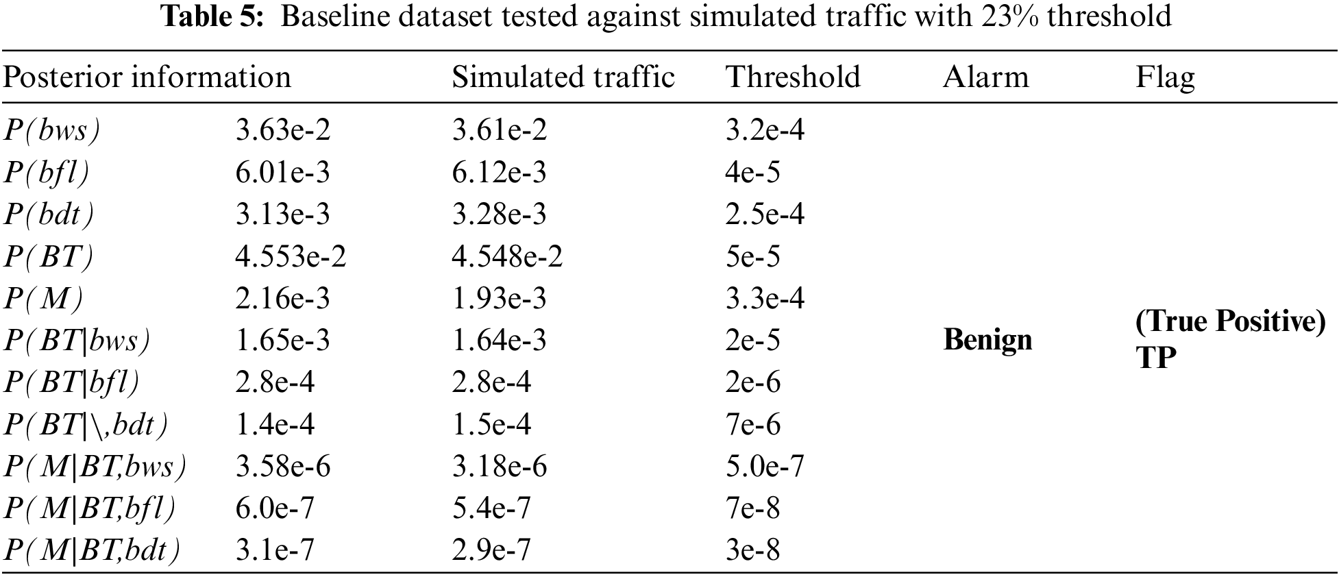
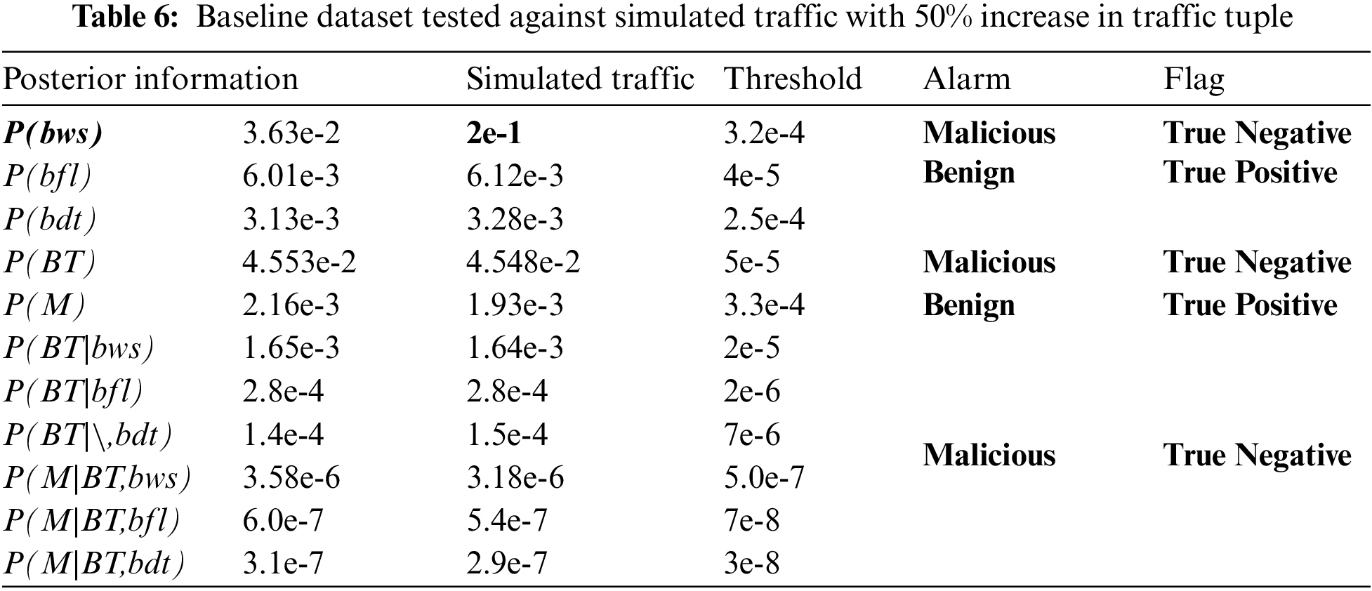
From Tab. 5, the threshold will flag more true positive traffic or simply true traffic. From here, the additional 23% traffic will still indicate 100% accuracy that all traffic is a true positive; with 100% detection rate and 0% false alarm rate. In the second and final scenario, this is where the amount of Pr (bws) of the simulated traffic (trained traffic) is increased by 50%. The results are as in Tab. 6.
A tuple of lambda Pr(bws) which is contained with malicious traffic had exceeded the threshold; a significant outcome . It will trigger the malicious alarm and it will be flagged as true negative traffic or simply true traffic. This will generate a bunch of true negative traffic based on the model. However, there are several tuples, which indicate a true positive traffic and this is true, as their lambda information does not exceed the threshold. This is considered a false alarm. To measure this, false alarm rate equation, which measures the false alarm over the whole traffic, is used. Here, the false alarm rate is at 27%. However, the detection rate (of detecting true traffic) is still at 73%; a significantly high probability rate.
4.3 Predictive Analysis Results Against Ground Truth Dataset
The next step is to use the optimized features and to fit it into the predictive analytics model as discussed in Stage 4 of the research activity. This model is used to test over the real use case scenario of an attacked dataset from the Malaysian healthcare provider as shown in Fig. 2 of Stage 4 of the research activity. The figure shows the testing dataset sampling extracted from the HGIGA® internet traffic utilization monitoring system dashboard. It also shows the attacked traffic were ranged from early May until early July 2017. Later attacked traffic will be set as a threshold value for the model. Traffic in August 2017 on the other hand was sampled as a baseline traffic. Traffic in October 2016 and early January 2017 will be studied to model its distribution.
The distribution characteristics of this testing traffic dataset were then recorded. The selected features were extracted during the feature selection phase and three optimized features were selected, namely λframe_len, for frame length lambda, λwin_size for window size lambda and λdelta_time for delta time lambda. These are the same selected features from the same feature selection model discussed in Stage 2 of the research activity.
The October traffic could be considered as benign traffic as it is way below the spike threshold. Generally, a threshold is used in many behavioral researches. For instance Weaver in [9] suggested that instead of hard setting the threshold heuristically, probabilistic relationship will give a more statistically rigorous outcome. Thus, in this research, the threshold is set by both probabilistic relationships and hard setting threshold. Hence, the quarter (¼) baseline rate was chosen to condition the prediction rate of more than 20% before the attack. In this section, the results have been discussed by applying the predictive model against the ground truth testing datasets. We run the dataset against our model and the result is summarized in Fig. 6. It is apparent that the proposed predictive analytics model has accurately detected a zero day attack a few months prior to the actual attack. For the baseline traffic of the ground truth dataset (October 2016), the model was already able to detect almost 60% of the traffic that was prepared for the zero day attack with 75% accuracy. Then the test traffic (January 2017), which was obtained five months prior to the attack, was run across the algorithm. The model has detected that 86% of the traffic was directed toward the attack and this time with 100% accuracy.

Figure 6: Predictive analytics model detection and accuracy rate
4.4 Results Against Other Classification Methods
Many researchers, for instance Leskovec in [25], considered Support Vector Machine (SVM) as a state-of-the-art classification method for behavioral malware analysis. Thus, the dataset is further trained, classified then later compared to the SVM model as defined in Eq. (29);
where XA and YA is the coordinate of point A and w is the weight vector. This is the margin between point A and the hyperplane. Each feature has a weight defined in Eq. (30);
where w is a distance inner product of some point A or the support vector with some point B along the hyperplane 90° to point A. In order to separate attack (1) from benign (0) episode is the work to decide the best separating line (hyperplane). Hence, there is a need to find the hyperplane with the largest margin; the line that separates ones and zeroes the most. The data are trained through total Least Squares residuals equation to obtain optimal hyperplane with optimal slope (m) and intercept (b). The general Least Squares (L) equation is defined in Eq. (31).
However, since support vector is used, the model is refined by measuring the Euclidean distance (D) of the support vector near the optimal hyperplane obtained from the Least Squares (L) model. Fig. 7 below is the depiction of the dataset separated by the optimal hyperplane.

Figure 7: A depiction of optimal hyperplane separating baseline traffic and attack traffic
Linear equation for the classification model mentioned in Eq. (28) will penalize the attacked nodes that fall into a normal region. This will determine the accuracy of the detection using this model. The measured accuracy is 5.83333e-1, which is almost 60% accuracy.
kNN (k Nearest Neighbor) is another classification and prediction model based on feature similarity of the nearest neighbors. This model is considered as the favorite model amongst researchers for its simplicity. Euclidean distance works in kNN algorithm. It determines the distance between the unknown data from all the points in the trained dataset. The closest distance from the nearest class neighbor will determine the class of the unknown dataset or test dataset. The binary classification and prediction model is derived from the general term of Euclidean Distance and extended into Eq. (32);
where

Figure 8: A depiction of test dataset separating baseline traffic and attack traffic using kNN
Tab. 7 summarizes the comparison results of the proposed model to other classification models discussed in this research. Again, detection rate and accuracy rate of the proposed Behavioral-based Malware Analysis model based on the Bayesian Network method scored 100% and 86%, significantly outperforming other models. False Alarm Rate also scored less, at 14% as compared to other classification models. This is achieved through the feature selection model and refined distribution model and finally the application of Bayesian Network for the classification model.

Acknowledgement: The authors wish to thank the Research Management Centre (RMC) of Universiti Teknologi MARA (UiTM), Universiti Kebangsaan Malaysia (UKM) and Centre for Languages and Foundation Studies (CELFOS), Universiti Sultan Azlan Shah (USAS).
Funding Statement: The work is fully sponsored by the research project grant FRGS/1/2021/ICT07/ UITM/02/3.
Conflicts of Interest: The authors declare that there are no conflicts of interest to report regarding the present study.
1. Z. K. Maseer, R. Yusof, S. A. Mostafa, N. Bahaman, O. Musa et al., “DeepIoT.IDS: Hybrid deep learning for enhancing IoT network intrusion detection,” CMC-Computers, Materials & Continua, vol. 69, no. 3, pp. 3945–3966, 2021. [Google Scholar]
2. O. A. Nojood, “A secure intrusion detection system in cyberphysical systems using a parameter-tuned deep-stacked autoencoder,” Computers, Materials & Continua, vol. 68, no. 3, pp. 3915–3929, 2021. [Google Scholar]
3. M. H. M. Yusof and A. M. Zin, “Network-level behavioral malware analysis model based on Bayesian network,” in Int. Conf. on Computer & Information Sciences (ICCOINS), Kuching, Malaysia, vol. 2021, pp. 316–321, 2021. [Google Scholar]
4. M. H. M. Yusof, “A review of predictive analytic applications of Bayesian network,” International Journal on Advanced Science, Engineering and Information Technology, vol. 6, no. 6, ISSN: 2088-5334, pp. 857–867, 2016. [Google Scholar]
5. H. Choi, M. Kim, G. Lee and W. Kim, “Unsupervised learning approach for network intrusion detection system using autoencoders,” The Journal of Supercomputing, vol. 75, no. 9, pp. 5597–5621, 2019. [Google Scholar]
6. L. A. Pereira, D. Taylor-Rodríguez and L. Gutiérrez, “A Bayesian nonparametric testing procedure for paired samples,” Journal of the International Biometric Society, vol. 76, no. 4, pp. 1133–1146, 2020. [Google Scholar]
7. Q. Li, F. Guo and I. Kim, “A non-parametric Bayesian change-point method for recurrent events,” The Journal of Statistical Computation and Simulation, vol. 90, no. 16, pp. 2929–2948, 2020. [Google Scholar]
8. M. H. M. Yusof, M. R. Mokhtar, A. M. Zin and C. Maple, “Embedded feature selection method for a network-level behavioural analysis detection model,” International Journal of Advanced Computer Science and Applications, vol. 9, no. 12, pp. 509–517, 2018. [Google Scholar]
9. R. Weaver, “Visualizing and modeling the scanning behavior of the Conficker botnet in the presence of user and network activity,” in IEEE TRANSACTIONS ON INFORMATION FORENSICS AND SECURITY, vol. 10, pp. 1039–1051, 2015. [Google Scholar]
10. K. Jiang, W. Wang, A. Wang and H. Wu, “Network intrusion detection combined hybrid sampling with deep hierarchical network,” IEEE Access, vol. 8, pp. 32464–32476, 2020. [Google Scholar]
11. P. Wang and Y. Z. Wang, “Malware behavioural detection and vaccine development by using a support vector model classifier,” Journal of Computer and System Sciences, vol. 81, no. 6, pp. 1012–1026, 2014. [Google Scholar]
12. G. Nguyen, S. Dluglinsky, V. Tran and A. L. Garcia, “Deep learning for proactive network monitoring and security protection,” IEEE Access, vol. 8, pp. 19696–19716, 2020. [Google Scholar]
13. F. Khan, A. Gumaei, A. Derhab and A. Hussain, “A novel two-stage deep learning model for efficient network intrusion detection,” IEEE Access, vol. 7, pp. 30373–30385, 2020. [Google Scholar]
14. P. Wei, Y. Li, Z. Zhang, T. Hu, Z. Li et al., “An optimization method for intrusion detection classification model based on deep belief network,” IEEE Access, vol. 7, pp. 87593–87605, 2019. [Google Scholar]
15. E. Ippoliti, “Heuristic reasoning: Studies in applied philosophy, epistemology and rational ethics,” in Springer International Publishing, Switzerland, pp. 1–2, 2015. [Google Scholar]
16. P. Fuster-Parra, P. Tauler, M. Bennasar-Veny, A. Ligeza, A. A. L´opez-Gonz´alez et al., “Bayesian network modeling: A case study of an epidemiologic system analysis of cardiovascular risk,” Computer Methods and Programs in Biomedicine, vol. 126, pp. 128–142, 2015. [Google Scholar]
17. T. Babu, D. Gupta, T. Singh, S. Hameed, M. Zakariah et al., “Robust magnification independent colon biopsy grading system over multiple data sources,” Computers, Materials & Continua, vol. 69, no. 1, pp. 99–128, 2021. [Google Scholar]
18. J. Yun, M. Basak and M. Han, “Bayesian rule modeling for interpretable mortality classification of COVID-19 patients,” CMC-Computers, Materials & Continua, vol. 69, no. 3, pp. 2827–2843, 2021. [Google Scholar]
19. M. Thangapandiyan and P. M. R. Anand, “An efficient botnet detection system for P2P botnet,” in Int. Conf. on Wireless Communications, Signal Processing and Networking (WiSPNET), Chennai, India, pp. 1217–1221, 2016. [Google Scholar]
20. B. Rahbarinia, R. Perdisci and M. Antonakakis, “Efficient behavior-based tracking of malware-control domains in large ISP networks,” in 45th Annual IEEE/IFIP Int. Conf. on Dependable Systems and Networks, Rio de Janeiro, Brazil, pp. 403–414, 2015. [Google Scholar]
21. M. A. Ambusaidi, H. Xiangjian, N. Priyadarsi and T. Zhiyuan, “Building an intrusion detection system using a filter-based feature selection algorithm,” IEEE Transactions on Computers, vol. 65, no. 10, pp. 2986–2998, 2016. [Google Scholar]
22. M. Hazewinkel, “Probability distribution,” in Encyclopedia of Mathematics, Dordrecht, Netherlands, 1994. [Google Scholar]
23. Y. Lei, “Intelligent fault diagnosis and remaining useful life prediction of rotating machinery,” in Elsevier Inc, United Kingdom, 2017. [Google Scholar]
24. I. Guyon and A. Elisseeff, “An introduction to variable and feature selection,” Journal of Machine Learning Research, vol. 3, no. 3, pp. 1157–1182, 2003. [Google Scholar]
25. J. Leskovec, A. Rajaraman and J. Ullman, “Mining of massive datasets: Support vector machines, Slides.” in Stanford University, California, United States, 2016. [Google Scholar]
 | This work is licensed under a Creative Commons Attribution 4.0 International License, which permits unrestricted use, distribution, and reproduction in any medium, provided the original work is properly cited. |