DOI:10.32604/cmc.2022.023947
| Computers, Materials & Continua DOI:10.32604/cmc.2022.023947 | |
| Article |
Internal Validity Index for Fuzzy Clustering Based on Relative Uncertainty
1Graduate School of Science Engineering & Technology, Istanbul Technical University, Istanbul, 34469, Turkey
2Faculty of Computer & Informatics, Istanbul Technical University, Istanbul, 34469, Turkey
*Corresponding Author: Refik Tanju Sirmen. Email: tsirmen@pirireis.edu.tr
Received: 27 September 2021; Accepted: 17 January 2022
Abstract: Unsupervised clustering and clustering validity are used as essential instruments of data analytics. Despite clustering being realized under uncertainty, validity indices do not deliver any quantitative evaluation of the uncertainties in the suggested partitionings. Also, validity measures may be biased towards the underlying clustering method. Moreover, neglecting a confidence requirement may result in over-partitioning. In the absence of an error estimate or a confidence parameter, probable clustering errors are forwarded to the later stages of the system. Whereas, having an uncertainty margin of the projected labeling can be very fruitful for many applications such as machine learning. Herein, the validity issue was approached through estimation of the uncertainty and a novel low complexity index proposed for fuzzy clustering. It involves only uni-dimensional membership weights, regardless of the data dimension, stipulates no specific distribution, and is independent of the underlying similarity measure. Inclusive tests and comparisons returned that it can reliably estimate the optimum number of partitions under different data distributions, besides behaving more robust to over partitioning. Also, in the comparative correlation analysis between true clustering error rates and some known internal validity indices, the suggested index exhibited the highest strong correlations. This relationship has been also proven stable through additional statistical acceptance tests. Thus the provided relative uncertainty measure can be used as a probable error estimate in the clustering as well. Besides, it is the only method known that can exclusively identify data points in dubiety and is adjustable according to the required confidence level.
Keywords: Machine learning; data science; clustering validity; fuzzy clustering; uncertainty; intelligent systems; data analytics
Clustering is a widely used interdisciplinary technique for classifying dimensional data objects by categorizing them into subsets based on specified similarity or dissimilarity measures. Due to it facilitates modeling and discovery of relevant knowledge in data [1] it is an essential part of many intelligent systems in vast areas, with a recognized prominence. Data analysis applications claim to explore multivariate real-life data of certain domains and extract hidden structures in them for various practices. Clustering is therefore one of the key methods of decision-making in machine learning as well [2].
There are diverse dichotomies in terms of clustering types, such as hard vs. soft, hierarchical vs. flat, model-based vs. cost-based, parametric vs. non-parametric, each with its implementations, serving different clustering aims [3]. These aims are worked to achieve through different algorithms that use relevant measures like inter-cluster separation, intra-cluster compactness, density, gap, normality, etc. Algorithms can comply with different approaches such as centroid-based k-means (cf. [4] for its origins), agglomerative hierarchical single [5] and complete linkage [6], spectral [7], mixture probability models [8,9], density-based DBSCAN [10], and so on.
Among a choice of algorithms, each with its relative advantages [11], fuzzy methods generalize hard-decision techniques by using fuzzy measures and distributing the membership degrees to each cluster [12,13]. This approach helps to deal with inexact systems by providing feasibility to utilize fuzzy outcomes and perform rule-based classifications. Continuous progress observed in the applications of this technology is evident. A wealth of material is available on the topic including [14–16].
Quite many of the ongoing efforts are on the analysis and improvement of the clustering accuracy, also on the complexity performances [17–20]. Some studies instead try to further explore the clustering theory, which could even serve to develop new approaches and algorithms. In [21], the statistical aspects of clustering are discussed and the focal questions are dealt with from the statistical perspective. Also [22] explains how correlation clustering can be a potent addition to data mining. Besides, the quality and efficiency are assessed and some useful metrics are suggested in several studies like [23–26].
Dependent largely on the structure of data, clusters obtained by a method may not necessarily be revealing for the respective application. Hence the validity of the partitioning needs to be evaluated so that the data model and the applied methods can be refined. As seen in Fig. 1 and also suggested in [27], cluster validation “should be part of any cluster analysis as integral to developing a classification model”.
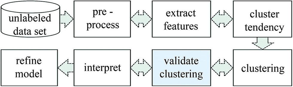
Figure 1: The ground of clustering validation
This quantitative evaluation process involves the following main issues: [27] a) Checking the randomness of the data, which can be determined by measuring cluster tendency. (Some measures such as Hopkins statistics, stability index, or some visual methods have been proposed to test the spatial randomness of the data [28–31]). b) Estimating the optimal number of clusters. c) Determining the compliance of the results to the data without any prior information. d) Comparing the results against an externally provided template. e) Comparing two sets of clusters to specify the relatively better one.
The first three tasks require unsupervised methods that use only the intrinsic information to be obtained from the data, thus called internal methods. In contrast, supervised methods deal with measuring how well the results fit the prespecified external information (typically class labels) not available in the data set. Rather than being a distinct type, relative methods are a special use of related measures, to compare results obtained from different methods or the same method with different parameters [27,32].
There are quite a few comparable internal and external methods and criteria that have been proposed to quantify validity. The validity function offered in [33] helps measure the cluster overlaps. The validity of a partition has also been discussed in many texts as [34] and an overall average compactness and separation measure was suggested for fuzzy clustering. Some works summarize, compare and evaluate the proposed validation measures from different aspects [35,36].
Since the ground truth reference is available in external validation, the decision of which clustering result is closer to the truth over a comparison criterion is independent of the underlying methods or data structures. Comparison criteria involve pair-counting and/or information-theoretic measures, entropy, purity, or the like which generally relate to diversity. Some recognized ones include the Jaccard coefficient [37], the Rand index [38], the adjusted Rand index [39], the adjusted mutual information [26] (better especially when dealing with unbalanced small clusters [40]), the Hubert statistics [40], and the principal component analysis based stability score [41]. In addition, [3] and [42] provide an overview of comparison criteria and their properties, and [26] specifically discusses some information-theoretic measures.
Internal indices on the other hand realize their evaluations in the absence of reference information about the data. Therefore, measures need to be devised from the data statistics. Hierarchical clustering schemes are mostly validated using the specific cophenetic correlation coefficient measure [43,44]. However, typical unsupervised measures for single schemes are compactness, which represents how cohesive the objects in a cluster are, separation, which represents how distinct one cluster is from the others, or a combination of these [27]. A vast literature is available explaining them with variations, such as [3,27,42]. Validity is determined through statistical hypothesis testing based on these criteria. Besides, the other major objective that internal indices serve is to estimate the optimum number of clusters, by testing a range of cluster counts and determining the number that best yields the criteria.
Validity indices specifically designed for fuzzy clustering calculate measures usually over fuzzy membership. While some require using also the data, others solely or mainly involve membership weights [45,46]. In this case, the sensitivity to the fuzzifier and the cluster count needs to be accounted for [3].
Some commonly used internal indices include Calinski et al. [47], Davies et al. [48], Silhouette [49], Xie et al. [34], Dunn's Index [50], and its modified versions such as Generalized [51], Alternative [52,53], and Modified [54] Dunn's Index. Further internal measures are discussed in [42]. Also in [55], 10 validity indices specifically for fuzzy clustering are reviewed.
1.2 Observations and Rationale
Validity indices competently deliver the essential inherent properties. Suggested methods measure the criteria through the inter-cluster and intra-cluster variances, entropies, and the like, evaluate the (dis)similarities, scrutinize the analysis as a whole, and then approximate the overall validity. However, it should be noted that the main clustering decisions may be made on some samples (the size issue), or distorted sets (the measuring-error issue). It was emphasized in [3] p.596 that, internal cluster validation “is more difficult than assessing the model fit or quality of prediction in regression or supervised classification, because in cluster analysis, normally true class information is not available”.
Unsupervised methods optimize their objective functions over the established criteria. Yet maybe such functions, to some extent, are measuring their conformity with the underlying clustering method, as much as the quality of the clustering result [56]. Moreover, a method may likely favor clusterings realized on the same criteria as itself. A detailed discussion on some validity indices that produce misleading results for the k-means algorithm on data with skewed distributions is presented in [42]. Also [57] shows that some analyzed indices were observed to be biased in certain conditions.
Furthermore, clustering is a classification kind process applied under uncertainty. Algorithms of the purpose are designed to partition given data, even though there should be no meaningful clusters in a random population [28], [31]. Since the number of partitions can theoretically go up to the number of data points, methods based mainly on improving (dis)similarity criteria by ignoring a confidence parameter may result in over-partitioning. Besides, in the validation of fuzzy clusterings, statistics of data points assigned with higher degrees of confidence have a subordinate relevance for credence, since they comprise limited information about uncertainty, that indeed appears in weakly assigned members.
Clustering is most probably part of a larger application. The decisive need in such an ambiguous case heavily based on statistics is a plausible method that estimates the probability margin of the anticipated actual error. In the absence of such an estimate, the resultant clustering has acquiesced as is. By with such a surmise, any probable clustering error would be dragged forward to the later stages of the system, regardless of the technique employed. Conversely, having such a measure of uncertainty, for a single observation or the whole clustering, would be very instrumental. Therefore, the accuracy performance of the performed clustering could be better approached by estimating the degree of uncertainty, apart from validity. Nevertheless, uncertainty and validity are not reciprocal.
From these, we can conclude that a labeling decision is, in a sense, a statistical test of the hypothesis that a sample data point comes from a particular cluster population at some level of confidence. Including a confidence level premeditated according to the application needs, therefore, reduces the inherent uncertainty in evaluations. As the term validation suggests, the correct estimation of optimal partitions is the premise of a valid clustering so that fewer labeling errors. Thus, a higher correlation between the measured validity index and actual clustering error rate indicates a stronger monotonic relationship.
Indeed respecting the fruitful efforts, revisiting the communal perception of the objective of validation in light of these considerations may be beneficial. As both intra-cluster similarity and inter-cluster dissimilarity increase, mean uncertainty in labeling should consequently decrease. Viz, the objective of clustering validation may be reformulated as minimizing the mean uncertainty in labeling assignments measured against defined criteria. Maximizing overall statistical confidence mathematically complies with maximizing the weights of the determined memberships in fuzzy clustering. This approach will also enable identifying data objects at dubiety state. The prominence of such information for other fields like machine learning is apparent.
This study tries to address these issues and suggests a purposive measure that provides an estimate for the level of uncertainty in realized fuzzy-family clusterings. The ensuing section reformulates the objective function as optimization of intra-cluster discordance and inter-cluster proximity, over uncertainties. The measure can be derived mainly by perusing weakly classified members’ appointed probability weights with a designated margin of confidence, as introduced below.
The method has been tested on numerous samples in diverse distributions and the results were compared with some well-known internal validity indices. An exclusive comparative analysis of the correlations between the indices and the measured actual clustering errors is also presented here. In addition, acceptance tests were applied to the obtained results as well, which are generally neglected.
In the remainder of this paper, Section 2 discusses the topic from the stated perspective, explains the envisaged methods, and introduces the proposed measures, Section 3 describes the details of the tests applied, including the acceptance tests, and Section 4 presents the obtained results. This is followed in Section 5 by the assessments and conclusions in respect to the canonical index properties set out.
Relying on the discussions so far, we can view the decision to label a sample data point into a particular cluster as a statistical test of the hypothesis that it comes from that cluster population at a certain level of confidence. Including the confidence level in evaluations will help manage inherent uncertainty in decisions. Established on this approach, the purpose of a validity index can be reformulated as minimizing mean uncertainty of the overall clustering process, measured on defined criteria.
The objective function of the proposed novel internal clustering validity index reaches its minimum at the point where compactness and separation of clusters are optimal, accorded by the given level of confidence. Below first the necessary definitions are provided within this framework of the relevant mathematical rationale. Then, the method is explained in detail, and its main advantages over other indexes are broadly highlighted.
2.1 Relative Uncertainty and Clustering
Clustering is a decision-making process under uncertainty relying on quantitative criteria. Under uncertainty, every observation is subject to distortion, by measurement errors and/or various interfering effects. The distance of observation to the sample mean i.e.,
As the expression (1) suggests, the δm decreases by Δm. To explore further, the commonly used k-means algorithm, as an example, tries to converge to local minima (through the Voronoi iteration) to reduce the sum of squared distances between the data points and the centroid [59]. Yet, the fuzzy c-means ‘FCM’ algorithm introduces the additional fuzzification exponent parameter that decides the level of cluster fuzziness [12,13]. By minimizing the objective function, the data points are associated with every cluster with mc weights (respecting the rule of Σmc = 1, 0 ≤ mc ≤ 1, 1 ≤ c ≤ k, k: number of clusters), as the m values indicate the membership probabilities. Ultimately the points are assigned to the clusters of the highest probabilities, i.e., mia = max (mic) is the assignment membership weight. The relevance of the assigned mia values depends on the decided number of clusters k and the distances to cluster centroids determined by the associated data points. Accordingly, as the accuracy of mia values enhances, the mean Δm, and correspondingly δm decreases, so does the mean relative uncertainty of the system.
The above remarks lead us to the hypothesis that when the data set is divided into the optimal number of clusters K and the points are labeled to establish this optimality, the overall relative uncertainty of the system is expected to be at a minimum. Therefore, the validity of clusterings can be estimated by measuring and comparing the total relative uncertainties. Furthermore, from the uncertainty perspective, the magnitude of the fuzzy assignment weight is statistically irrelevant, as long as it satisfies the desired confidence level. Hence the question of validity can be reformulated as, whether the hypothesis that the data points truly come from the associated cluster populations proves, at a certain level of confidence. As with the number of assumed partitions k can theoretically go up to the number of data points n, it can be suspected that basing the validity method solely on improving similarity and dissimilarity criteria ignoring the confidence and uncertainty parameters may lead to over-partitioning, defined as k > K.
This requires designating an interval that specifies the upper and lower margins of error, for a given confidence level. Moreover, for our topic, a weight beyond the upper bound is an indication that no cluster other than the one yielding the highest probability is close enough to be graded (i.e., a strong membership). Therefore, we only need to consider here the lower bound when determining uncertainties. Any association below this bound can be assumed weak and thus uncertain.
2.2 Uncertainty Boundary and Weak Members
The m probabilities essentially depend on the intra-cluster and inter-cluster variances (i.e., the compactness, and separation). Due to numerous detrimental effects, data points may shift too close to a neighbor cluster's boundary, which could cause labeling errors. Such 2 points are marked in Fig. 2. Here a 3D example reference space is assumed, which can be easily abstracted to N dimensions. Different colors represent different clusters. The da and dn are the vectorial distances of the points on the similarity measure to the assigned and the next-most-probable clusters’ centroids cia and cin respectively. That means, for data point i, dia = || i–cia || and din = || i–cin ||.
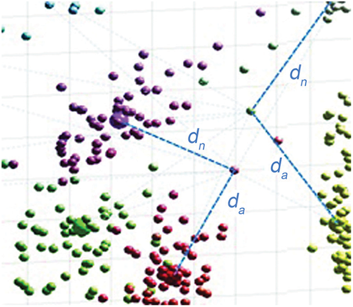
Figure 2: Peripheral weak members
The members on the periphery of a cluster are the ones being under the most risk of incorrect labeling if there exists another cluster too close. Ipso facto, such weak members are assigned with lower m weights. Deciding an uncertainty boundary (will be denoted by δb) gives us the capability of classifying the members assigned with lower weights as weak members. Say {w} represents the weak-members set. Then a data point i with an assignment (i.e., the maximum) membership weight mia less than δb is to be identified as a weak member. Below the expression (2) provides the formal definition of a weak member.
The compactness of every cluster could vary due to different distribution effects, so a -roughly derived- overall δb would be misleading. Thus uncertainty boundaries should be exclusively computed on a per-cluster basis for the desired confidence level (which is 1–α), and the weak members are identified in accordance. Eq. (3) gives the general formula of the uncertainty boundary. Here μm and σm represent the mean and standard deviation of m weights, zα is the reference z-score for designated confidence (1–α), and n is the number of members.
2.3 Dubiety Boundary and Members in Dubiety
When all data points of a cluster are right at their centroids then μ(da) and σ(da) should return zero. For all cases other than this theoretical one, μ(da) > 0. On the other hand, if dia/din = 1 then the point i is at the limbus since it is at an equal distance to both centroids as expression (4) depicts. The limbo state manifests the highest level of uncertainty.
In the ‘FCM’ algorithm [12,13], the membership weight mia of data point i in the cluster a is defined as below in Eq. (5) (k: number of clusters, ca, cc: centroids, e: fuzzification exponent):
In this equation, ||i-ca|| and ||i-cc|| are essentially consistent with the above-mentioned distances. Then, dia/dic gives the proportion of the distances to different cluster centroids. As this proportion gets closer to 1, the anticipated confidence level in the classification decision for point i decreases. Correspondingly, let us say mia and min be the maximum and the next highest fuzzy membership weights of i respectively. So,
A proximity value γ close to 1 in Eq. (6) indicates that it is not clear which cluster the data point belongs to (which corresponds to the case of a Silhouette index close to zero). Analogous to Eq. (2), if represents the set of members in dubiety state, we can designate the members, as in Eq. (7):
This means that cluster members with γi values less than or equal to the dubiety boundary constitute the set of members in dubiety state adjacent to other clusters. The following definition formally provides a generic boundary to identify data points in dubiety state, with the foregoing ‘limbus’ at the lowest end.
Based on Chebyshev's inequality, the probability of the observations being r standard deviations away from the mean is at least (1 – 1/r2) [58]. Eq. (9) justifies the dubiety boundary definition in Eq. (8).
Hence, proximity values lower than or equal to
2.4 The Relative Uncertainty Index of Clustering
The optimal number of partitions (K) of a given dataset at the desired level of confidence is expected to achieve where the overall uncertainty rate is minimum. Theoretically, k can go up to n as it is presumed that the data set is suitable for partitioning.1 So, the relative uncertainty index (that will be referred to as ‘rU’ hereafter) for k partitions can be formulated as in Eqs. (10) and (11):
Here, πc and γc respectively denote the discordance (as the opposite of coherence) and proximity (as the opposite of separation) of cluster c. Thus the objective function is to minimize the rUk value as in Eq. (11). The cluster discordance can be computed through Eqs. (12) and (13) given below.
δba and nc are the uncertainty boundary and the number of members of the cluster c. Also, tα is the student's t-value corresponding to α, and sma is the standard deviation of ma values (i.e., normalized mia weights, please cf. Eq. (19)) for cluster members. Since (
On the other hand, referring to Eq. (6), cluster proximity based on uncertainties can be computed as:
Like δba in Eq. (13), δbn in Eq. (18) is the adjacency boundary for the mi values (i.e., normalized min weights, cf. Eq. (19)), and smn is the standard deviation of mn values. So in Eqs. (16) and (17), ma < δba for data point i indicates that i is in the weak members set {wc}, and similarly if mn > δbn it is in the adjacency set {ac}. Union of them constitutes the proximity set {γc} of cluster c defined in Eq. (15). The mean of the γi matrix of {γc} members thus corresponds to the average separation from nearest clusters, i.e., Eq. (14) (np is the set members count).
An important issue to note is that all of the raw mia and min membership weights must be normalized first by their standard deviations as described in Eq. (19) below (where mix here denotes mia or min) to make the cluster-wise calculations invariant to the k changes. Such normalization makes all membership values more robust to their monotonic dependence on k and sensitivity to the fuzzification exponent, so that serves to prevent under partitioning by using the same order of magnitudes. (A section is devoted to the importance and effects of measure normalization in [42].)
In epitome, the unitless relative uncertainty index rUk provides a blind estimate of the average relative uncertainty of the fuzzy clustering operation for k partitions. The optimum number of partitions K is the k where rUk reaches its minimum, by minimizing the πc while maximizing the γc.
It should be heeded that being the desired confidence level (1–α) can be set gives the additional ability to adjust the index according to the respective application. Moreover, besides providing an estimation of the optimum number of partitions, the presented ‘rU’ index can specifically identify members in dubiety and the weak members of each cluster (via Eq. (7), and Eq. (16)).
Some desirable properties of an internal validity index can be deemed as follows:
• Reliability: A reliable index is expected to yield consistent results on data with as many different underlying frequency distributions as possible, without assuming Gaussian or such.
• Validity: Under and over partitioning would result in higher clustering errors. As the title suggests, the correct estimation of optimal k is the premise of valid clustering, so then fewer labeling errors. Hence, the calculated index is expected to correlate with measured true clustering errors.
• Robustness to over-partitioning: Since unsupervised methods attempt to partition data even it does not contain any clusters, the need to priorly apply cluster tendency tests arises [28,31]. Thus, over (and under) partitioning is a threat the index should avoid.
• Independence of measure: With no stipulation on the measure (as Euclidean, Mahalanobis, or such), it is supposed to run independently of the underlying similarity measure.
• Informativeness: Calculation outcomes can be elucidative on intrinsic statistics of the data to serve further scopes.
• Optimality: Deriving adequate internal statistics from a sample set rather than the entire population data (which may not always be possible) is desirable. This practice would mean lower time and memory complexities.
• Efficiency: Another creditable property is the efficiency of the index, mainly in terms of time complexity, which may become quite significant especially in real-time applications.
Numerous diverse tests were conducted mainly towards these canonical properties we suggest, and the results were also compared with some of the well-known internal validity indices, as shared below. Another point worth mentioning is that acceptance tests as well, which are mostly neglected, were applied to the results obtained under different conditions. Tests are explained in the ensuing sections.
The tests were performed on various numeric structural data both artificially generated 2 as well as retrieved from online repositories (e.g., http://cs.joensuu.fi/sipu/datasets, https://www.kaggle.com/datasets, https://data.world/datasets/clustering, http://archive.ics.uci.edu/ml, with files such as S2, S3 [61], A1, A2 [62], Mall_Customers.csv, etc.). 3 Being the test data in different distributions was particularly mulled.
Clustering was carried out using the ‘FCM’ algorithm, with random initiation. A non-partial clustering was assumed, thus no group was left empty when all of the points were eventually assigned. Also, the data was assumed non-overlapping, so then the data points were associated with the cluster of the highest membership probability. The fuzzification exponent parameter was 2.0, the minimum improvement per iteration was 10−6, and the maximum number of iterations was 200. Parameters were selected in common standards for all subjects, as no significant effects were observed on validation tests.
For all cases, validity metrics were computed for the ‘rU’ index, as well as 8 additional well-known internal indices, namely Calinski-Harabasz, Davies-Bouldin, Silhouette, Dunn, Alternative, Generalized, and Modified Dunn, besides Xie-Beni. (Abbreviations CH, DB, S, D, AD, GD, MD, XB are used to respectively stand for these indices throughout this text.) Every set was tested at least 35 times for each K, as incrementing n in steps of 25. Besides, the whole clustering and index computation process was repeated at least 25 times before determining the optimal k on average, to avoid the possible effect of the random initiation in the ‘FCM’.
For correlation analysis, additional artificial noisy data sets were generated in Gaussian, Weibull, and Poisson probability density distributions (each with K = 8, n > 600), for Gaussians to represent the middle, and the other 2 represent two possible extremes. Various tests were conducted on at least 600 different sets for every noise environment.
Correlation coefficients were computed to scrutinize the strength of the relationship between the relative behaviors of the measured accuracy performances and the validity indices including rU. The specified confidence level for correlation was 95% during the tests, and the maximum acceptable performance error was FPr < 0.05 (please see the related title below).
Pearson's product-moment correlation coefficients were assumed principal, yet Spearman's rank correlation coefficients were evaluated as well. Computed coefficient magnitudes were interpreted as ± r2 indicating: .0--.19: very weak, .20--.39: weak, .40--.59: moderate, .60--.79: strong, .80--1.0: very strong [63].
Clustering accuracy performance was measured by comparing the estimated and provided ground-truth labels using two external indices depicted below:
• FPr: The false-positive clustering error rate ‘FPr’ identifies the rate of false-positive (FP) mappings obtained from the comparisons that can be stated as in Eq. (20) (cio is the original ground-truth label, cia is the assigned label, and n is the number of data points in the population).
When a complete (i.e., non-partial) clustering was assumed, as all of the points got assigned, no group was left empty. Since we were to compare against the ground-truth partitions, a non-overlapping point could not belong to more than one group simultaneously, and it is eventually assigned to a particular one, because of the complete clustering assumption. This means an FP assignment that occurred in some cluster should be the concurrent counterpart of a false-negative (FN) assignment in another cluster, and under these conditions, ΣFP = ΣFN.
• aRI: To cover the overlaps, also the Adjusted-Rand index [40] was computed, which is a version of the Rand index adjusted for chance, as described in [38].
Even if significant correlation coefficients satisfying the confidence level were observed in all studied environments, the significance of the differences between the correlation coefficients obtained in different environments should also be tested before the correlation can be eventually accepted. (We encourage to confer to [64].) Hence, the hypotheses have been established to test the significance of the differences as H0: ρ1 – ρ2 = 0 and H1: ρ1 – ρ2 > 0 (ρ being the correlation coefficient).
Since the sample populations were gathered from three principal environments (namely Gaussian, Poisson, and Weibull), the tests were conducted for every pair, let's say ρg-ρp, ρp-ρw, and ρg-ρw. Afterward, if all three of the pairwise tests returned that the H0 was not rejected at the desired level of confidence then the consistency of the correlation decision was accepted for that variable; it was rejected otherwise.
For the null-hypothesis tests, the criterion of significance was assumed as 0.05 (i.e., zα = 1.96). The tests were applied separately both to the attained Pearson and Spearman correlation coefficients for every variable in question. Pairwise z-scores zgp, zpw, zgw were computed and compared with the reference z-score zα. In conclusion, if zxy < zα then the null hypothesis could not be rejected at the specified level of confidence, thus the differences between the predictive values were not of significance. (Note that attaining all 6 separate zxy < zα results was mandatory for accepting the consistency of a single variable.)
The collected results from the tests are summarized and discussed below.
The optimum number of partitions k estimations by the proposed ‘rU’ index were quite consistent with the other indices. Fig. 3 exemplifies divergences between k-estimates and true K on 148 samples of D = 2, 160 ≤ n ≤ 480, 3 ≤ K ≤ 15, in different distributions. The bars indicate the absolute mean divergence percentages of K estimations from the true K.
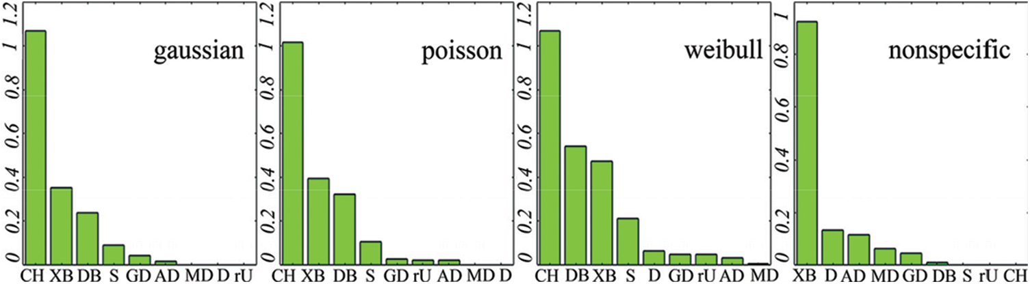
Figure 3: K-k divergences
However, peculiar cases that deserve to be marked were also observed. Fig. 4 (left-hand side) shows some sample data (D = 2, n = 160, K = 4) in clusters using different colors (Red crosses point the centroids; the weak members are marked with magenta circles, and members in dubiety with black diamonds). On the right-hand side, the optimum number of partitions estimated by the indices is marked with red circles (occurring at the minimum or maximum depending on the objective function of the related index).
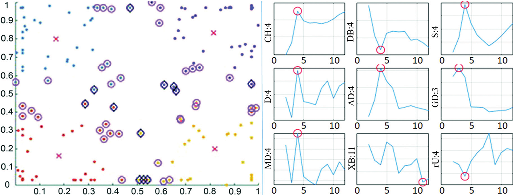
Figure 4: Clustering and K estimations of data set m2_4_160
In this example, almost all tested indices correctly estimated the designed 4 partitions when examined within the range of 2 < k < 12. However, most indices returned higher estimates when the inspection window was expanded, as pictured in Fig. 5. The left-hand side of the figure shows the estimations for the range of 2–22, while the right-hand side shows the range of 2–74. Even occasionally, more than 1 local optimum may appear (as can be seen with the ‘D’ and ‘MD’ indices in k: 2–22 range).
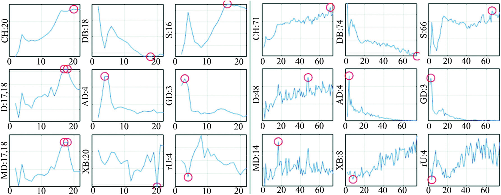
Figure 5: Over partitioning of m2_4_160
Several such peculiarities were encountered during tests. This observation tells that even if the optimum K value can be accurately determined within a given range, over partitioning can occur when the range is expended without considering the uncertainties in the putative clusters.
Conducted tests to explore relationships between the considered indices and the true errors returned various levels of correlations, as listed in Tab. 1 (G, P, and W respectively denote the Gaussian, Poisson, and Weibull distribution environments). As it can be noticed in the table, the proposed ‘rU’ index exhibited the highest (very strong) correlations among all in each noise environment tested.

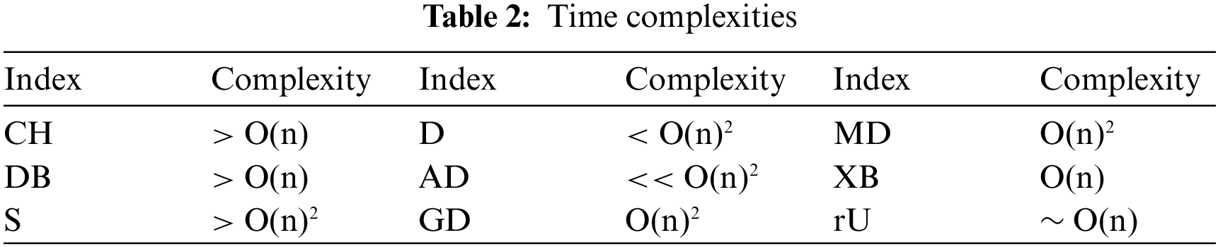
The ‘rU’ index uses only the membership weights, while many of the others need to reach the data itself. It can be counted as a benefit in terms of memory requirements. Besides, performing primary calculations only on the weak members also marks the additional optimality of the ‘rU’. This optimality reflects on the time complexity as, the ‘rU’ index involves only the uni-dimensional 1st and 2nd level membership weight matrices for the calculations, regardless of the data dimension. Hence the time complexity of distance calculations, such as compactness and separation, increases at some indices according to the data dimension, while in the ‘rU’ it remains monotonically dependent only on the size.
Tab. 2 implies that the time complexity of the ‘rU’ is considerably better compared to many [51,54,65]. Consequently, observed run times vindicated the relative efficiency of the ‘rU’. While the ‘S’ index exhibited the far worst runtimes of all, the ‘XB’ yielded faster processing than the ‘rU’, yet it showed weaker correlations with the measured clustering errors, besides failed in the acceptance tests.
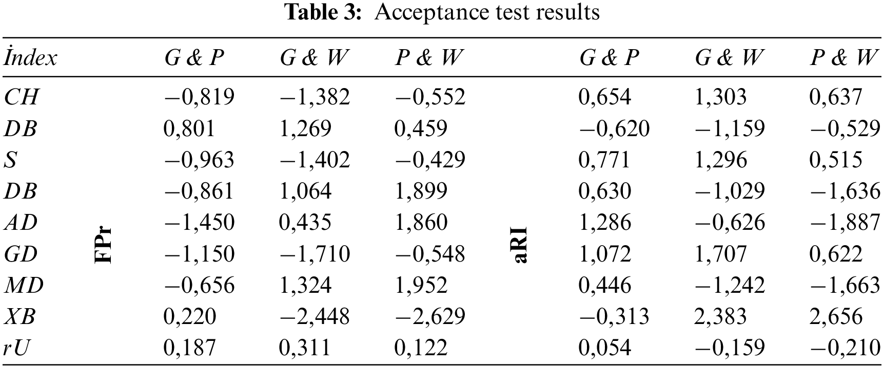
It was also observed that the ‘rU’ index passed all acceptance tests, while the Xie-Beni index failed in some cases due to higher z-differences over the critical value (z = 1.96), as seen in Tab. 3. This casts doubt that such indices may be likely to exhibit instabilities on some data distributions.
The prevalence of research on clustering and cluster validation, which are among the essential tools of data analytics, reveals the importance of the topic. Although the clustering process is exercised under uncertainty, and validity indices provide explanatory insights into the intrinsic properties of the data, they do not deliver any quantitative assessment of the possible uncertainties in the realized partitioning. They may also be biased because they measure, to some extent, their conformity with the underlying clustering criteria. Several studies report such misleading results. Besides, it is also observed that ignoring the required confidence level may lead to over partitioning. On the other hand, considering a confidence parameter can reduce the risk of over partitioning, thereby better preventing potential errors from being carried towards subsequent phases of applications like machine learning where clustering is likely a part of. Moreover, having an uncertainty estimation can be also utilized to refine predictive functions.
In light of these motivations, this study mainly focuses on clustering validation and proposes a novel internal method designed specifically for fuzzy clustering, based on relative uncertainty. Through discussions of the “validity of validation” itself, it incorporates the confidence parameter to the evaluation of criteria and reestablishes the objective as optimization of the level of uncertainty. To this end, here introduced the mathematical definition of weak members, as well as the method of estimating uncertainty, apart from validity. The method is independent of size, underlying density distribution, similarity measure, or clustering algorithm that membership weights are obtained with.
The proposed relative uncertainty index, named ‘rU’, satisfies all canonical aspects of an unsupervised validity measure. Inclusive tests and comparisons have shown that it can reliably estimate the optimum number of partitions in different data distributions without stipulating Gaussian or any other and it is comparatively robust to over partitioning. It uses only one-dimensional membership weights regardless of the data dimensions, similarity measure, and the like. The impact of the resultant low complexity from this optimality has also been positively observed in runtime efficiencies.
A competent clustering validity measure is expected to correlate with true error rates. Relevant tests have also shown the highest strong correlations between true error statistics and the ‘rU’ index in all test environments, compared to the others. This relationship has been proven consistent through statistical acceptance tests as well, which is mostly neglected.
Along with the mentioned contributions, it is probably the first fuzzy validation measure adjustable to the application needs, as includes the confidence parameter in the evaluation. The uncertainty measure as an error probability estimate can be used as a metric as well, in the credence of the realized fuzzy clustering. Another significant novelty that can be quite instrumental for tuning the later stages of the system involved is the ability to exclusively identify the weak members in the designated clusters.
The efficacy of the proposed method is most likely to manifest itself especially with unbalanced or distorted distributions with higher uncertainty. However, the fact that it was specially designed for fuzzy clustering should be noted as a limitation. Besides, datasets more suitable for hierarchical clustering need to be studied separately. A further research opportunity opened is associating the provided uncertainty estimate to an appertaining cost function for incorporating the risk assessment into classification decision rules. Also, designing a layered iterative classification algorithm that makes use of the diagnosis of weak members is another promising future work.
1It may be necessary to decide on cluster tendency first (please cf. related references in the previous section).
2The datasets generated during the current study are available from the corresponding author upon request.
3Specifics of the test data were 2 ≤ D ≤ 13 (one with D=912), 50 ≤ n ≤ 5250, 3 ≤ K ≤ 35 (where ‘D’, ‘n’, and ‘K’ here respectively represent dimension, size, and numberof designed partitions), in distributions Gaussian, Poisson, Weibull, Nonspecific.
Acknowledgement: The authors would like to thank the editors for reviewing this manuscript.
Funding Statement: The authors received no specific funding for this study.
Conflicts of Interest: The authors declare that they have no conflicts of interest to report regarding the present study.
1. F. Azuaje, W. Dubitzky, N. Black and K. Adamson, “Discovering relevance knowledge in data: A growing cell structures approach,” IEEE Transactions on Systems, Man, and Cybernetics, Part B, vol. 30, no. 3, pp. 448–460, 2000. [Google Scholar]
2. S. Shalev-Shwartz and S. Ben-David, in Understanding Machine Learning: From theory to algorithms, Cambridge University Press, NY, USA, pp. 307–327, 2014. [Google Scholar]
3. C. Hennig and M. Meila, “Cluster analysis: An overview,” In: C. Hennig, M. Meila, F. Murtagh and R. Rocci. (Eds.). in Handbook of Cluster Analysis, CRC, Taylor & Francis, FL, USA, pp. 1–20, 2016. [Google Scholar]
4. H. -H. Bock, “Origins and extensions of the k-means algorithm in cluster analysis,” Electronic Journal for History of Probability and Statistics, vol. 4, no. 2, pp. 1–18, 2008. [Google Scholar]
5. K. Florek, J. Lukaszewicz, J. Perkal, H. Steinhaus and S. Zubrzycki, “Sur la liaison et la division des points d'un ensemble fini,” Colloquium Mathematicum (Wrocław), vol. 2, no. 3-4, pp. 282–285, 1951. [Google Scholar]
6. G. N. Lance and W. T. Williams, “A general theory of classificatory sorting strategies: 1. hierarchical systems,” The Computer Journal, vol. 9, no. 4, pp. 373–380, 1967. [Google Scholar]
7. J. Shi and J. Malik, “Normalized cuts and image segmentation,” IEEE Transactions on Pattern Analysis and Machine Intelligence, vol. 22, no. 8, pp. 888–905, 2000. [Google Scholar]
8. B. G. Lindsay, “Mixture models: Theory, geometry and applications,” in American Statistical Association in Hayward, Institute of Mathematical Statistics, CA, USA, vol. 5, pp. 1–163, 1995. [Google Scholar]
9. S. Richardson and P. J. Green, “On bayesian analysis of mixtures with an unknown number of components,” Journal of the Royal Statistics Society, vol. Series B 59, pp. 731–792, 1997. [Google Scholar]
10. M. Ester, H. P. Kriegel, J. Sander and X. Xu, “A density-based algorithm for discovering clusters in large spatial databases with noise,” in Proc. of 2nd Int. Conf. on Knowledge Discovery and Data Mining, Portland, OR, USA, pp. 226–231, 1996. [Google Scholar]
11. P. Nerurkar, A. Shirke, M. Chandane and S. Bhirud, “Empirical analysis of data clustering algorithms,” Procedia Computer Science, vol. 125, pp. 770–779, 2018. [Google Scholar]
12. J. C. Dunn, “A fuzzy relative of the ISODATA process and its use in detecting compact well-separated clusters,” Cybernetics and Systems, vol. 3, no. 3, pp. 32–57, 1973. [Google Scholar]
13. J. C. Bezdek, Pattern Recognition with Fuzzy Objective Function Algorithms, NY, USA: Plenum Press, 1981. [Google Scholar]
14. J. V. Oliveira and W. Pedrycz, Advances in Fuzzy Clustering and its Applications, NY: Wiley, pp. 3–28, 2007. [Google Scholar]
15. G. Gan, C. Ma and J. Wu, “Data clustering: Theory, algorithms, and applications,” in ASA-SIAM Series on Statistics and Applied Probability, SIAM, Philadelphia, ASA, Alexandria, VA, pp. 151–159, 2007. [Google Scholar]
16. J. Han, M. Kamber and J. Pei, Data Mining: Concepts and Techniques, 3rd ed., San Francisco, USA: Morgan Kaufmann Publishers, pp. 426–429, 2012. [Google Scholar]
17. M. T. Gallegos and G. Ritter, “Strong consistency of k-parameters clustering,” Journal of Multivariate Analysis, vol. 118, pp. 14–31, 2013. [Google Scholar]
18. S. Clémençon, “A statistical view of clustering performance through the theory of U-processes,” Elsevier Journal of Multivariate Analysis, vol. 124, pp. 42–56, 2014. [Google Scholar]
19. M. Alata, M. Molhim and A. Ramini, “Optimizing of fuzzy c-means clustering algorithm using GA,” International Journal of Computer and Information Engineering, vol. 2, no. 3, pp. 670–675, 2008. [Google Scholar]
20. R. Nock and F. Nielsen, “On weighting clustering,” IEEE Transactions on Pattern Analysis & Machine Intelligence, vol. 28, no. 8, pp. 1223–1235, 2006. [Google Scholar]
21. U. V. Luxburg and S. Ben-David, “Towards a statistical theory of clustering,” In Proc. Pascal Workshop on Statistics and Optimization of Clustering, London, UK, pp. 20–26, 2005. [Google Scholar]
22. F. Bonchi, D. García-Soriano and E. Liberty, “Correlation clustering from theory to practice,” in Proc. of 20th ACM SIGKDD Int. Conf. on Knowledge Discovery and Data Mining, NY, USA, pp. 1972, 2014. [Google Scholar]
23. C. Alexander and S. Akhmametyeva, “The shape metric for clustering algorithms,” arXiv, Computer Science, Mathematics, vol. 1807.08524v1, pp. 1–10, 2018. [Google Scholar]
24. C. Alexander and S. Akhmametyeva, “A family of metrics for clustering algorithms,” arXiv, Computer Science, Mathematics, vol. 1807.08912v1, pp. 1–16, 2018. [Google Scholar]
25. S. Chormunge and S. Lena, “Metric based performance analysis of clustering algorithms for high dimensional data,” in Proc. of 5th Int. Conf. on Comm. Syst & Network Technologies, Gwalior, India, pp. 1060–1064, 2015. [Google Scholar]
26. N. X. Vinh, J. Epps and J. Bailey, “Information theoretic measures for clusterings comparison: Variants, properties, normalization and correction for chance,” The Journal of Machine Learning Research, vol. 11, pp. 2837–2854, 2010. [Google Scholar]
27. P. N. Tan, M. Steinbach and V. Kumar, “Introduction to data mining,” in Addison Wesley, Longman Publishing Co., Inc., MA, USA, pp. 532, 2005. [Google Scholar]
28. D. Kumar and J. C. Bezdek, “Visual approaches for exploratory data analysis: A survey of the visual assessment of clustering tendency (VAT) family of algorithms,” IEEE Systems, Man and Cybernetics Magazine, vol. 6, no. 2, pp. 10–48, 2020. [Google Scholar]
29. K. R. Prasad and B. E. Reddy, “Assessment of clustering tendency through progressive random sampling and graph-based clustering results,” in 3rd IEEE Int. Advance Computing Conf., Ghaziabad, India, pp. 726–731, 2013. [Google Scholar]
30. B. Hopkins and J. G. Skellam, “A new method for determining the type of distribution of plant individuals,” Annals of Botany, New Series, vol. 18, no. 70, pp. 213–227, 1954. [Google Scholar]
31. R. G. Lawson and P. C. Jurs, “New index for clustering tendency and its application to chemical problems,” Journal of Chemical Information and Computer Sciences, vol. 30, (no. 1,pp. 36–41, 1990. [Google Scholar]
32. M. Halkidi, M. Vazirgiannis and C. Hennig, “Method-independent indices for cluster validation and estimating the number of clusters.,” In: C. Hennig, M. Meila, F. Murtagh, R. Rocci (Eds.in Handbook of Cluster Analysis. CRC, NY, USA: Taylor & Francis, pp. 595–618, 2015. [Google Scholar]
33. J. C. Bezdek, “Numerical taxonomy with fuzzy sets,” J. of Mathematical Biology, vol. 1, pp. 57–71, 1974. [Google Scholar]
34. X. L. Xie and G. Beni, “A validity measure for fuzzy clustering,” IEEE Transactions on Pattern Analysis and Machine Intelligence, vol. 13, no. 8, pp. 841–847, 1991. [Google Scholar]
35. Y. Liu, Z. Li, H. Xiong, X. Gao and J. Wu, “Understanding of internal clustering validation measures,” in Proc. of IEEE Int. Conf. on Data Mining, Atlantic City, NJ, USA, pp. 911–916, 2010. [Google Scholar]
36. J. Hämäläinen, S. Jauhiainen and T. Kärkkäinen, “Comparison of internal clustering validation indices for prototype-based clustering,” MDPI Algorithms, vol. 10, no. 3, pp. 105, 2018. [Google Scholar]
37. P. Jaccard, “The distribution of flora in the alpine zone.1,” New Phytologist, vol. 11, no. 2, pp. 37–50, 1912. [Google Scholar]
38. W. M. Rand, “Objective criteria for the evaluation of clustering methods,” Journal of the American Statistics Association, vol. 66, no. 336, pp. 846–850, 1971. [Google Scholar]
39. S. Romano, N. X. Vinh, J. Bailey and K. Verspoor, “Adjusting for chance clustering comparison measures,” Journal of Machine Learning Research, vol. 17, pp. 1–32, 2016. [Google Scholar]
40. L. Hubert and P. Arabie, “Comparing partitions,” Journal of Classification, vol. 2, no. 1, pp. 193–218, 1985. [Google Scholar]
41. A. Ben-Hur and I. Guyon, “Detecting stable clusters using principal component analysis,” Methods in Molecular Biology, vol. 224, pp. 159–182, 2003. [Google Scholar]
42. H. Xiong and A. Li, “Clustering validation measures,” In: C.C. Aggarwal, C.K. Reddy (Eds.in Data Clustering Algorithms and Applications, CRC, NY, USA: Taylor & Francis, pp. 571–606, 2014. [Google Scholar]
43. J. S. Farris, “On the cophenetic correlation coefficient,” Systematic Zoology, vol. 18, no. 3, pp. 279–285, 1969. [Google Scholar]
44. S. Saracli, N. Dogan and I. Dogan, “Comparison of hierarchical cluster analysis methods by cophenetic correlation,” Journal of Inequalities and Applications, vol. 2013, pp. 1–8, 2013. [Google Scholar]
45. W. Wang and Y. Zhang, “On fuzzy cluster validity indices,” Fuzzy Sets and Systems, vol. 158, no. 19, pp. 2095–2117, 2007. [Google Scholar]
46. M. Falasconi, A. Gutierrez, M. Pardo, G. Sberveglieri and S. Marco, “A stability based validity method for fuzzy clustering,” Pattern Recognition, vol. 43, no. 4, pp. 1292–1305, 2010. [Google Scholar]
47. T. Calinski and J. Harabasz, “A dendrite method for cluster analysis,” Communications in Statistics, vol. 3, no. 1, pp. 1–27, 1974. [Google Scholar]
48. D. L. Davies and D. W. Bouldin, “A cluster separation measure,” IEEE Transactions on Pattern Analysis and Machine Intelligence, vol. PAMI-1, no. 2, pp. 224–227, 1979. [Google Scholar]
49. P. J. Rousseeuw, “Silhouettes: A graphical aid to the interpretation and validation of cluster analysis,” Computational and Applied Mathematics, vol. 20, pp. 53–65, 1987. [Google Scholar]
50. J. C. Dunn, “Well separated clusters and optimal fuzzy partitions,” Cybernetics, vol. 4, no. 1, pp. 95–104, 1974. [Google Scholar]
51. N. R. Pal and J. Biswas, “Cluster validation using graph theoretic concepts,” Pattern Recognition, vol. 30, no. 6, pp. 847–857, 1997. [Google Scholar]
52. B. Balasko, J. Abonyi and B. Feil, Fuzzy Clustering and Data Analysis Toolbox for use with Matlab, Veszprem, Hungary: University of Veszprem, 2005. [Online]. Available: https://www.researchgate.net. [Google Scholar]
53. I. Shafi, J. Ahmad, S. Shah, A. Ikram, A. A. Khan et al., “Validity-guided fuzzy clustering evaluation for neural network-based time-frequency reassignment,” EURASIP Journal on Advances in Signal Processing, vol. 2010, no no. 636858, pp. 1–14, 2010. [Google Scholar]
54. N. Ilc, “Modified dunn's cluster validity index based on graph theory,” Przeglad Elektrotechniczny, Electrical Review 2, vol. 2012, pp. 126–131, 2012. [Google Scholar]
55. M. H. F. Zarandi1, M. R. Faraji and M. Karbasian, “An exponential cluster validity index for fuzzy clustering with crisp and fuzzy data,” Scientia Iranica, vol. 12, no. 7, pp. 95–110, 2010. [Google Scholar]
56. R. Feldman and J. Sanger, The Text Mining Handbook: Advanced Approaches in Analyzing Unstructured Data, NY, USA: Cambridge University Press, 2007. [Google Scholar]
57. M. Kim and R. S. Ramakrishna, “New indices for cluster validity assessment,” Pattern Recognition Letters, vol. 26, no. 15, pp. 2353–2363, 2005. [Google Scholar]
58. M. Rouaud, “Probability, statistics and estimation: Propagation of uncertainties in experimental measurement,” 2017. [Online]. Available: http://www.incertitudes.fr/book.pdf. [Google Scholar]
59. S. P. Lloyd, “Least squares quantization in PCM,” IEEE Transactions on Information Theory, vol. 28, no. 2, pp. 129–137, 1982. [Google Scholar]
60. F. Pavlovčič, J. Nastran and D. Nedeljković, “Determining the 95% confidence interval of arbitrary non-Gaussian probability distributions,” in Proc. of XIX IMEKO World Congress Fundamental and Applied Metrology, Lisbon, Portugal, pp. 2338–2342, 2009. [Google Scholar]
61. P. Fränti and O. Virmajoki, “Iterative shrinking method for clustering problems,” Pattern Recognition, vol. 39, no. 5, pp. 761–775, 2006. [Google Scholar]
62. I. Kärkkäinen and P. Fränti, “A dynamic local search algorithm for the clustering problem,” in Research Report University of Joensuu, Joensuu, Finland, vol. A, no. A-2002-6, pp. 1–11, 2002. [Google Scholar]
63. K. J. Worsley, S. Marrett, P. Neelin, A. C. Vandal, K. J. Friston et al., “A unified statistical approach for determining significant signals in images of cerebral activation,” Human Brain Mapping, vol. 4, no. 1, pp. 58–73, 1996. [Google Scholar]
64. F. E. Croxton, B. W. Bolch and D. J. Cowden, in Practical Business Statistics, 4th ed., NJ, USA: Prentice-Hall, pp. 218–222, 1969. [Google Scholar]
65. S. Zhou, F. Liu and W. Song, “Estimating the optimal number of clusters via internal validity index,” Neural Process Letters, vol. 2021, no. 53, pp. 1013–1034, 2021. [Google Scholar]
 | This work is licensed under a Creative Commons Attribution 4.0 International License, which permits unrestricted use, distribution, and reproduction in any medium, provided the original work is properly cited. |