DOI:10.32604/cmc.2022.024417
| Computers, Materials & Continua DOI:10.32604/cmc.2022.024417 | |
| Article |
Scaled Dilation of DropBlock Optimization in Convolutional Neural Network for Fungus Classification
Signal Processing Research Laboratory, Department of Electronics and Telecommunication Engineering, Rajamangala University of Technology Thanyaburi, Pathum Thani, Thailand
*Corresponding Author: Jakkree Srinonchat. Email: jakkree.s@en.rmutt.ac.th
Received: 16 October 2021; Accepted: 13 February 2022
Abstract: Image classification always has open challenges for computer vision research. Nowadays, deep learning has promoted the development of this field, especially in Convolutional Neural Networks (CNNs). This article proposes the development of efficiently scaled dilation of DropBlock optimization in CNNs for the fungus classification, which there are five species in this experiment. The proposed technique adjusts the convolution size at 35, 45, and 60 with the max-polling size 2 × 2. The CNNs models are also designed in 12 models with the different BlockSizes and KeepProp. The proposed techniques provide maximum accuracy of 98.30% for the training set. Moreover, three accurate models, called Precision, Recall, and F1-score, are employed to measure the testing set. The experiment results expose that the proposed models achieve to classify the fungus and provide an excellent accuracy compared with the previous techniques. Furthermore, the proposed techniques can reduce the CNNs structure layer, directly affecting resource and time computation.
Keywords: DropBlock; convolutional neural network; deep learning; fungus classification
Fungus is one type of microorganism that plays an essential role in ecology and currently has more than 100,000 species [1,2]. Its growth exists, maintains, and spreads in the terrible weather, causing diseases to plants, animals, and humans. Infection from fungus is named “mycoses.” There are two types of mycoses in humans: superficial mycoses infected from various species [3–6] and systemic mycoses [7–10]. There are primary process methods to classify the mycoses species, such as matrix-assisted laser desorption/ionization time-of-flight mass spectrometry and polymerase chain reaction to assess the presence of other candida albicans and aspergillus under aerobic conditions [11], open-ended coaxial probe in couple with the microwave analysis to identify the fungus electrical properties [12]. Though such approaches give reliable and precise results, they need special devices that are costly and require well-trained practitioners to operate. Thus, this is the medical limitation to analyzing and identifying the disease's causing the spreading and growth are speedy. Therefore, computer vision and deep learning techniques are the alternative solutions to get quick and efficient results. The development of computer vision in couple with deep learning comprises many processes, such as data access via a microscope and mathematical methods to explain the structure and identification of species. From such processes, some studies and development, as shown in [13], presented the Bottom-hat and Otsu’ Threshold technique to enhance the sharpness and separate the material on the image and artificial neural networks (ANNs) with a total of 30 nodes that were classified fungus spores. The experiment results indicated 93.6% of the efficiency. Those researches were exciting because the development aimed to resolve the problem of identifying the fungus species. From the guidelines, the development has been continued. As shown in [14], the Support Vector Machine (SVM) technique to detect the fundus was proposed. The research set two dominant features of fungus, Hand-crafted, and Histogram of Oriented Gradients. The experiment compared the feature map, size [2 × 2], [4 × 4], and [8 × 8], which were the images used in the learning with the SVM technique. The experiment results showed that the accuracy efficiency was 88% and 70%. The Convolutional Neural Network model consisted of 10 layers, with the 2 × 2 convolution windows and the 3 × 3 kennel [2]. The softmax function was the final part of the network, which was to receive the neurons. The experiment is based on the learning rate (LR) at 0.1 to 0.00001. The fungus spore database used for the training and experiment comprised 5 species, 40,800 images, of which 30,000 images were for the training set and 10,800 images for the experiment set. The image size was adjusted to 76 × 76 pixels to increase the training speed. The experiment results showed 94.8% of accuracy efficiency. The [15] presented a web application. The research emphasized the dominant feature of the chemical culture color, whereas the experiment technique focused on transferring the ResNet 50 model. In training, the determination of learning rate was 0.0001, Adam optimizer (β1) was 0.9, Adam optimizer (β2) was 0.999, Adam minibatch size was 128, and Max epoch was 1000 rounds. The accuracy efficiency of the results was 96.5%. Moreover, in [16], the research proposed enhancing CNNs model efficiency and the morphology technique. The accuracy efficiency of the experiment was 93.26%. In [17], the research proposed comparing new CNNs, including RCNN, VGG-19, Le-Net, and Inception-V3. Such a model utilized 36,486 images in the training and experiment. The efficiency of the experiment was 93.6% (R-CNN), 91.2% (VGG-19), 81.0% (Le-Net) and 93.1% (Inception-V3). Furthermore, the [18] was experimented by transferring the learning by emphasizing the Resnet-C-SVM training model with 1,204 images. The accuracy efficiency of training results was 96.5%. [19] showed the efficiency comparison of GoolgeNet and AlexNet model, which were tested with the database of Aspergillus, 40,000 images. The accuracy efficiency of the experiment results was 95% and 96%. Moreover, [20] illustrated the fungus classification using the parameter of SVM (Kernel, C, RBF) in couple with AlexNet, InceptionV3, and ResNet 18. The database was divided into 2 sets involving 2-fold cross-validation and 5-fold cross-validation. The efficiency of experiment results was 82.4% ± 0.2% and 93.9 ± 3.9% (AlexNet FV SVM), 41.3% ± 1.9% and 55.0% ± 5.6% (InceptionV3 FV SVM), 71.3% ± 1.5% and 88.3% ± 2.7% (ResNet18 FV SVM). The feature extraction and classification network expansion with 16 layers consisting of convolution, kernel, pooling, and the full connection is presented [21]. The training included 1,500 images of fungus. The efficiency of the experiment results was 98.03% (accuracy). In [22], the research proposed fine-grained multi-instance-based deep attention. The model utilized 2,000 images in the training and experiment. The efficiency of the experiment was 94.3% (accuracy). The results were concluded in Tab. 1.
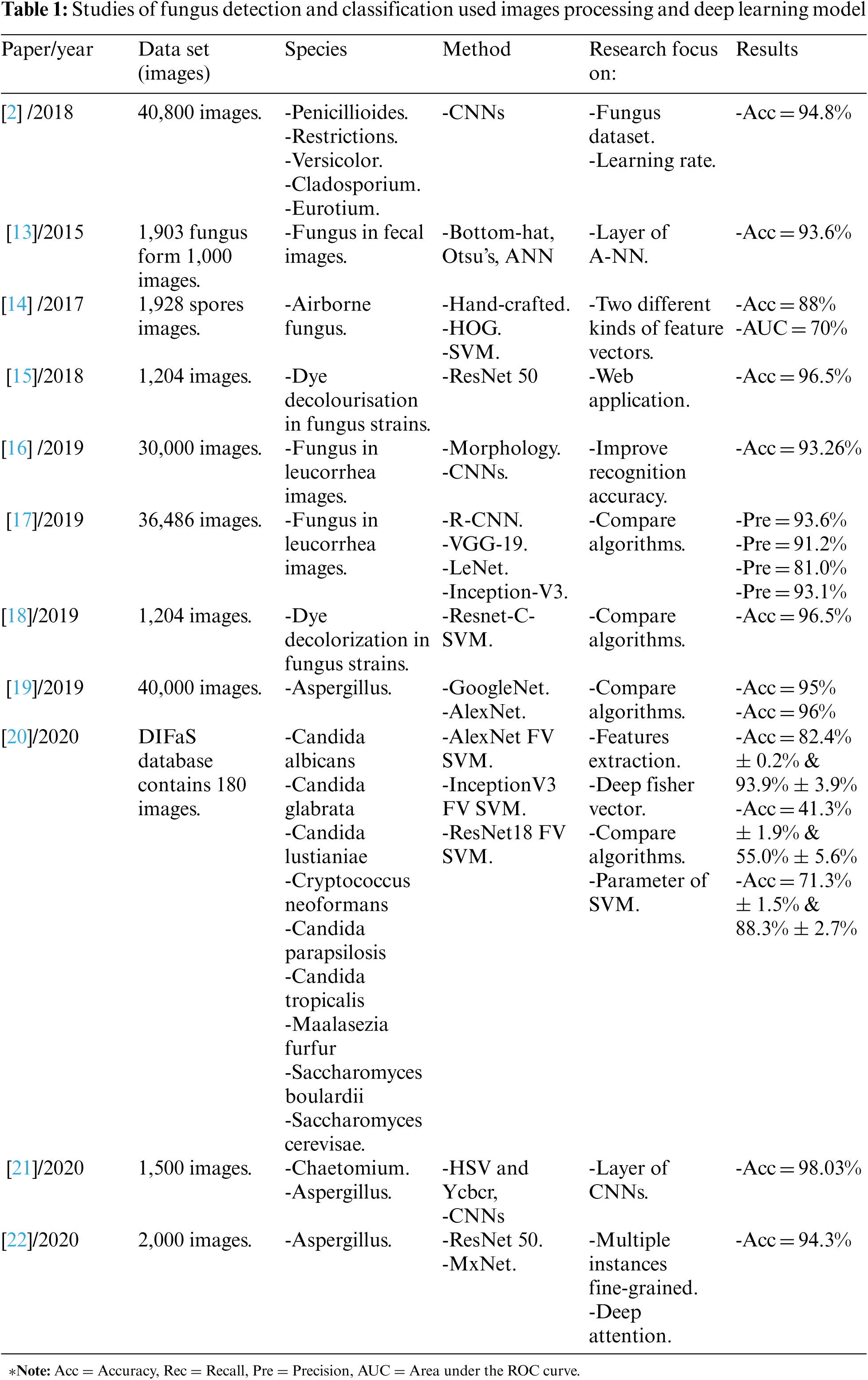
It can notice in Tab. 1 that most of the previous deep learning techniques for fungus classification adjusted parameters and kernel size of the convolutional layers, which were the significant factors of the feature extraction. Thus, this research aims to improve the efficiency of the CNNs models by adjusting the convolutional net with adjusting the BZ and KP of DropBlock parameter for fungus classification that can apply to the biotechnical. Those fungi consist of Aspergillus, Absidia, Fusarium, Penicillium, Rhizopus with metula, phialide, conidium, sporangium as physical features. The performance of the proposed models is measured using precision, recall, f1-score, and confusion matrix. The rest of this paper is organized as follows: Section 2 experimental method setup and fungus datasets are presented; the result in Section 3; the discussion in Section 4; Section 5 conclusion our findings and future work.
As shown in Fig. 1, the overview of the research was divided into three parts. Firstly, it was the access to fungus images. It involved sample collection, microscope observation, and data synthesis (rotation, contrast, refection, and gaussian noise). Secondly, the convolution structure extracted the network components into three parts; the first was feature extraction. This research included the Convolution, max-pooling, and DropBlock, respectively, as shown in Tab. 2. This research modified the stack to maximize the capability to feature extraction (shape, line, and colors). The second part was the activation function that decides the final value of a layer, which replaces all negative values to zero and remains the same with the positive values. Finally, in the third part, the researcher modified the wholly connected layers to increase the network's learning. Such layers were standardized by applying the dropout to improve the solution's efficiency. This network was trained with the learning function to enhance the capability of feature learning, which the learning rate was not modified during the training and the training number. However, it focuses on the efficiently scaled dilation of BZ and KP, which were the crucial part of the features extraction and the experimental method to determine the optimal efficiency of the model. Finally, the accuracy, recall, precision, and f1-score are also used to evaluate the classification performance.
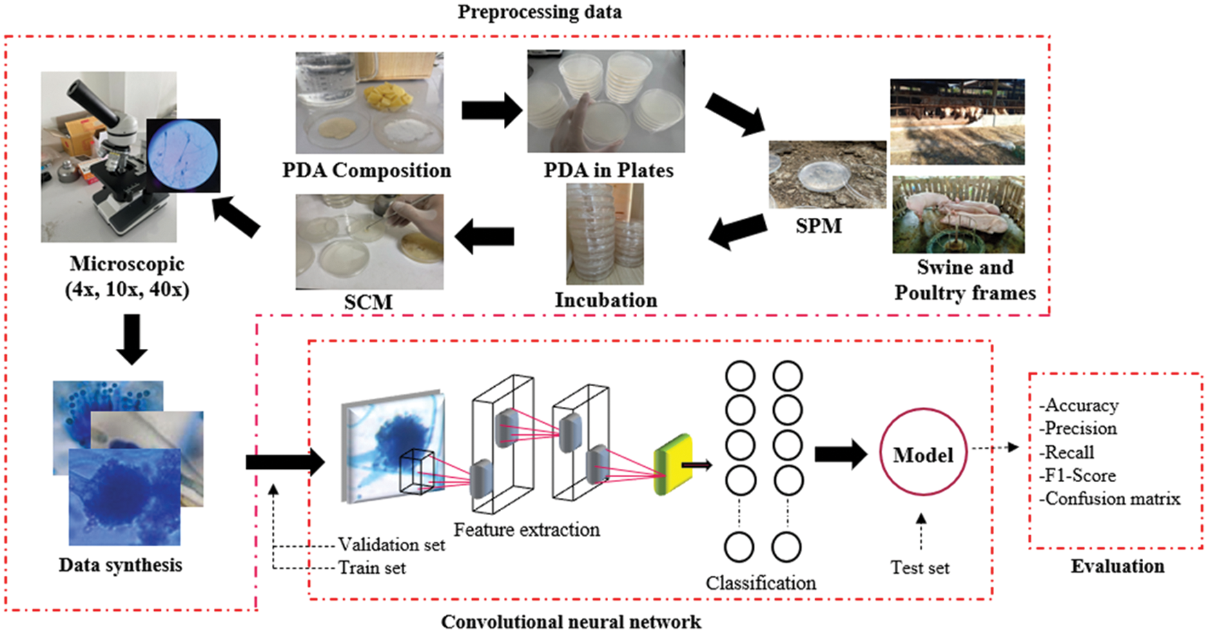
Figure 1: The proposed method for fungus classification
This research collected the sample using the settle plate method (SPM). The 36 petri plates with the culture medium, potato dextrose ager (PDA), were placed at 9 spots around the swine and poultry farms without disturbing activity, 4 replicating each area. Left the plates for 30 min and incubated at room temperature for 4 days. After using the slide culture method (SCM) for preparing fungus colonies for examination and identification, incubation temperature at 25°C–28°C, 4 or more days. The colonies were collected from such an approach, as shown in Fig. 2.
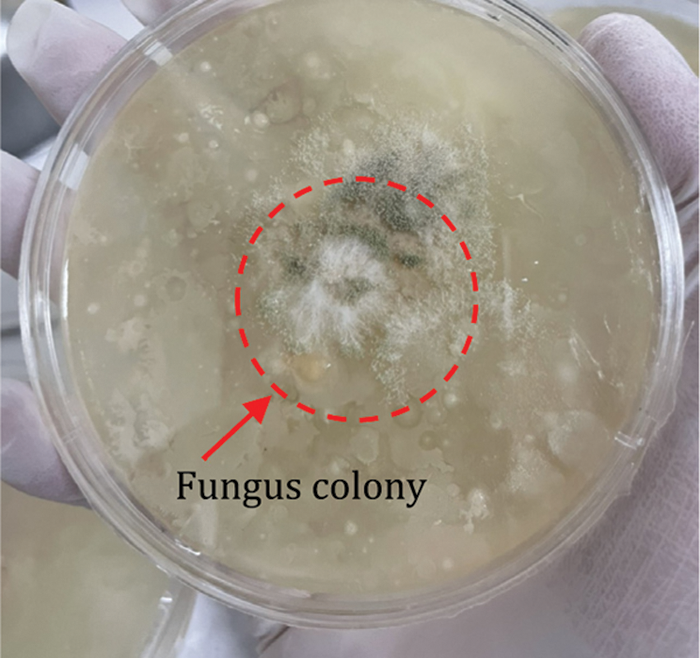
Figure 2: The colonies of fungus on petri plates
The explanation of each colony was introduced in [23–26]. Then, it raked the colony with Lactophenol Cotton Blue (LPCB), as shown in Fig. 3a. The images were collected via the XENON SME-F1L microscope with the magnification 4x, 10x, and 40x, as shown in Fig. 3b. Then, it cropped only the fungus area, which was 359 images in total, including 84 images of Aspergillus (Asp), 77 images of Absidia (Abs), 72 images of Fusarium (Fus), 61 images of Penicillium (Pen), and 65 images of Rhizopus (Rhi). The number of such images was limited when counting as the image for training deep learning.
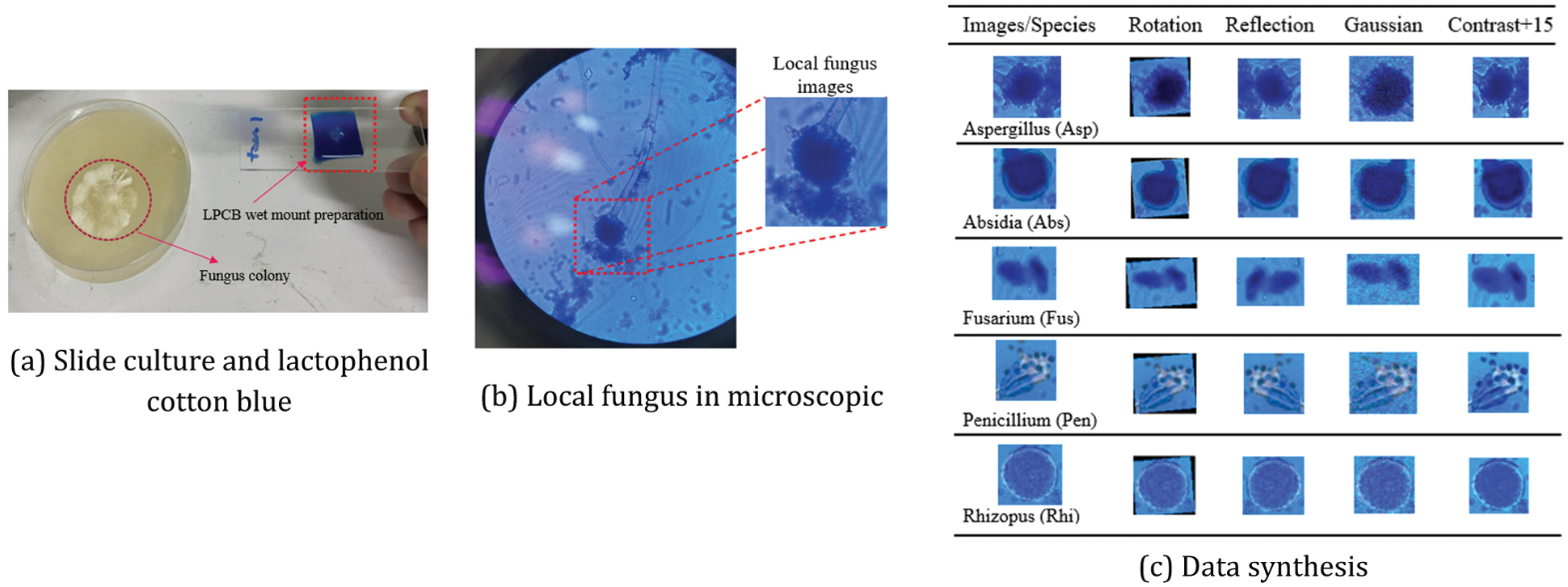
Figure 3: Local fungus images in microscopic and data synthesis
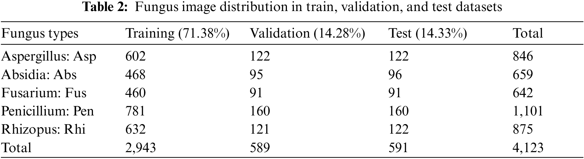
The images are converted with the rotation, refection, histogram balance adjustment or contrast, and gaussian noise in the data synthesis step in [27], as shown in Fig. 3c. It was proved that such an approach was reliable and straightforward, which could be applied to the variable image and the top view vision. The number of images was concluded in Tab. 2.
An amount number of five fungus species images is shown in Tab. 2. It can create a category to be training set, validation set, and testing set approximately 72%, 14%, and 14%, respectively.
2.2 Convolutional Neural Network
The convolutional neural network (CNNs) architecture had been developed to recognize the form and classify the data [28]. The neural network with the order of feature extraction functioned with the classification to resolve the traditional technique; setting the extent of pixel movement on the image as desired resulted in the inefficient outcome. On the other hand, the CNNs technique applied the feature extraction from the convolution and connected layers, which functioned as the encoder. Currently, it could be used widely, such as image division or object detection. As mentioned earlier, CNNs proved that it provided efficient results for medical research. For example, CNNs was applied to classify lung disease, identify cancer on CT [29], detect malaria parasites [30], fecal examination, and COVID-19 test [31].
Moreover, the model structure of CNNs had been developed to be compatible with the various data, such as ResNet [15], VGG Net [17], and GoogleLeNet [19]. However, such a model had a limited size, structure, filtration layer, parameter, and input layer size to the database dimension. The large-sized model required time to train and learn with the specific data which the transfer learning (TL) [18] was one of the exciting approaches to resolve such problems.
The critical components of CNNs consisted of the 3 parts:
The first part was the convolutional stage which classified the data components, such as the edge of object, shape, and color. The filter was created to verify such components, which could be calculated with Eq. (1), where Z was the kernel of the image I.
The second part was the detector stage, which was necessary for the network extraction. Rectified Linear Unit (ReLU) was the popular function because of its ability to change the negative component of the matrix to 0 while maintaining other values. The researcher added it to the feature extraction and classification stage, calculated with Eq. (2), where x was the output activation. From the component equation for feature filtration, ReLU was the popular activation function due to its ability to change the negative component of the matrix to 0 while maintaining other positive values.
From (1)-(2), the kernel's weight was used with the input image, so it extracted the high quality of the specific position depending on the size of the kernel. ReLU left the gap for feature classification, and the output from the convolution was always higher than the input. Finally, the pooling stage determined the maximum value at the position where the filter overlapped, and it cooperated with the determined stride. Then, the data would be sent to the classification layer.
In addition, the efficiency of convolutional layers is continuously increased by the Dropout (DO) [32] or Spatial Dropout (SDO) [33], which had been proved that they could enhance the model efficiency. However, the results were unsatisfactory when applied to the image data because the feature extraction randomized the image with a high relationship. Therefore, such an approach extracted the area components inefficiently. Consequently, it could not send the features to the next layer. Thus, this proposed technique exploits the DropBlock [34] to solve these problems. The BlockSize (BZ) and γ are two crucial parameters in which BZ is the drop area, and γ is the unit controller of dropping. Also, the KeepProp (KP) is the unit operation probability during dropout state, as shown in Eq. (3).
The third part was the classification stage, which received the input from the convolution layer. The input changed to vector and calculated using the Eq. (4) that the neuron's information was
Anyhow, the Softmax function was the function to receive the total of classification layers. This research put it at the last layer of the network to make the output in the probability to calculate the negative probability for the loss of cross-entropy where the total value was 1 or 1 approaches value, as shown in Eq. (5):
This research presented the CNNs in couple with the DB optimized. The details of the network are shown in Tab. 3. The total proposed structure consisted of 32 layers, divided into 15 convolutional layers, 5 DB layers, 5 max-pooling layers, 1 flatten layer, and 4 fully connected layers (4 dense layers, 2 dropout layers, 1 softmax activation). The ReLu activation function was used in this setup. Regarding the feature extraction, the kernel was different at each layer; max-pooling was in the size of 2 × 2 with SAME and Padding to move the filter's position and increase the gap for the extraction. All layers had the ReLu activation to minimize the vanishing gradient problem, so quickly processing the training. The DB layer was behind the feature extraction layer to emphasize the image quality. Regarding the classification, ReLu activation was the total result function with the dropout (0.20) to screen the node. The softmax function was in the last layer to receive the complete results of the classification.
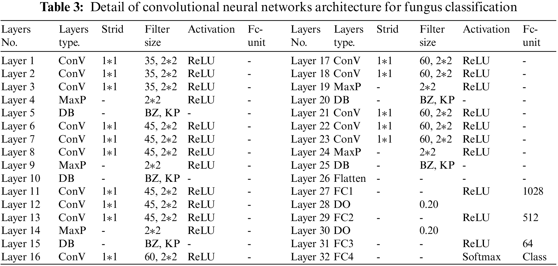
The VGG Net inspired the proposed components. The model included the convolution layers to classify the features at different levels, emphasizing feature extraction to obtain the utmost data. The experiment applied the convolutional sizes 35, 45, and 60 with the max-pooling sized 2 × 2 and the DB, which significantly enhanced the model efficiency. All factors were connected, so the calculation was reasonable.
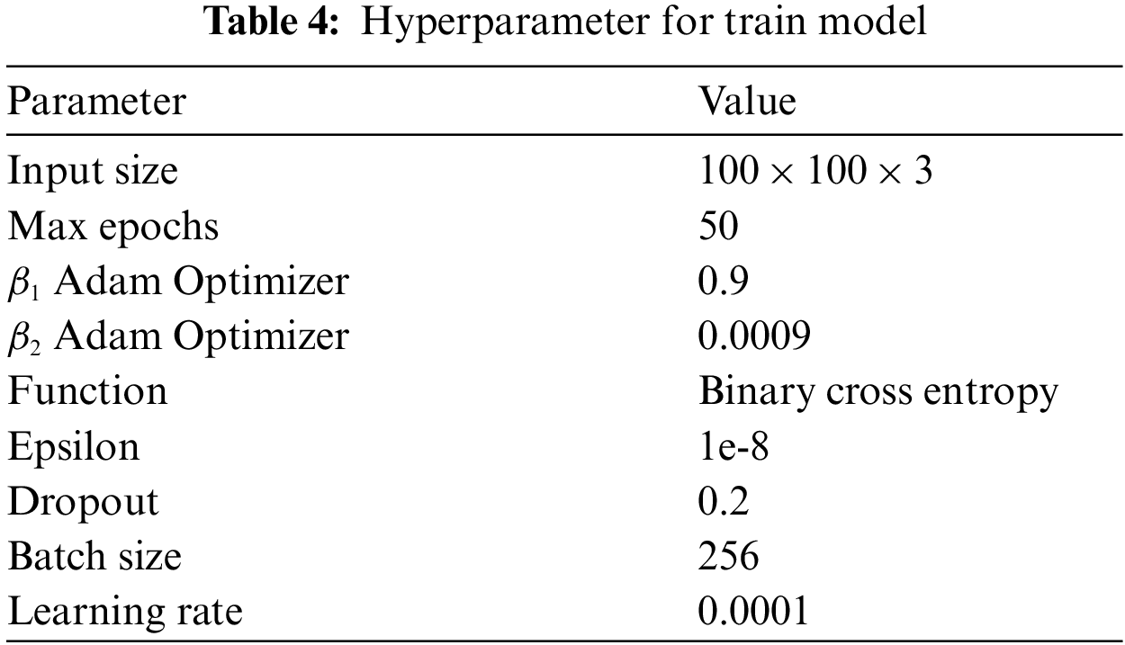
The proposed architecture was tested with the image sized 100 × 100 × 3 pixel and trained with the model 50 times. During the training, the learning rate was adjusted to 0.0001 while the Adam Optimizer was set at 0.9 (β1) and 0.0009 (β2). The learning function binary cross-entropy model used the ReLU function to compile a feature where the softmax function was in the last layer of the classification. The batch size for classifying the data in training was set at 256, with the epsilon set at 1e-8. The detail of the parameter was concluded in Tab. 4.
This experiment was performed on Windows 10 and the graphic processing on NVidia GeForce RTX 2070 Super Gaming OC 8 GB with the memory at 32 GB to accelerate the calculation speed. For the DL technique, the researcher applied the library of Tensorflow and Keras. The fungus image retrieval from OpenCV depended on Python 3.6.
The research on DL was divided into 2 main groups to resolve the regression and classification problems. This research presented a CNNs model to classify the fungus image. The model's efficiency was measured from the variable y with the value from 0 to 1. The research results were calculated from the accuracy as the Eq. (6) to evaluate model performance. In fungus types, precision, recall, and f1-score as the Eqs. (7)-(9) are considered evaluation metrics for classifier performance.
In the experiment, the BZ and KP are modified to investigate the suitable feature map in the decision function. The modification can be divided into 2 types. Firstly, in the term of vary BZ, the parameter of BZ adjusted to 1, 4, 6, 8, 10, and 12, respectively, and the parameter of KP was the static value at 0.99. The accuracy efficiency of training results was 95.56%, 97.13%, 96.48%, 98.30%, 97.04%, and 97.60%, as shown in Fig. 4a. The val_accuracy efficiency was 99.22, 99.89, 97.32, 99.89, 99.78, and 100.0, as shown in Fig. 4b. Secondly, in the term, vary BZ and KP, the parameter of BZ was random as 4, 3, 2, 7, 1, and 11, and the parameter of KP was also random 0.61, 0.72, 0.58, 0.70, 0.65, and 0.81, respectively. The accuracy efficiency of training results was 94.36, 87.05, 87.75, 96 .01, 91.66, and 96.99, as shown in Fig. 4c. The val_accuracy efficiency was 48.83, 66.69, 47.94, 66.89, 70.01, and 94.54, as shown in Fig. 4d. Finally, this research model was performed with the test set. The fungus classification results and the confusion matrix were shown in Tab. 5 and Fig. 5, respectively.
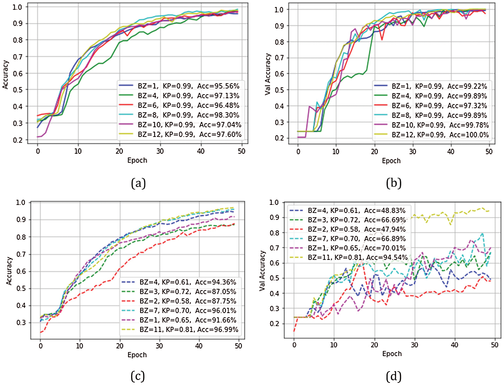
Figure 4: The performance of accuracy and validation of CNNs model
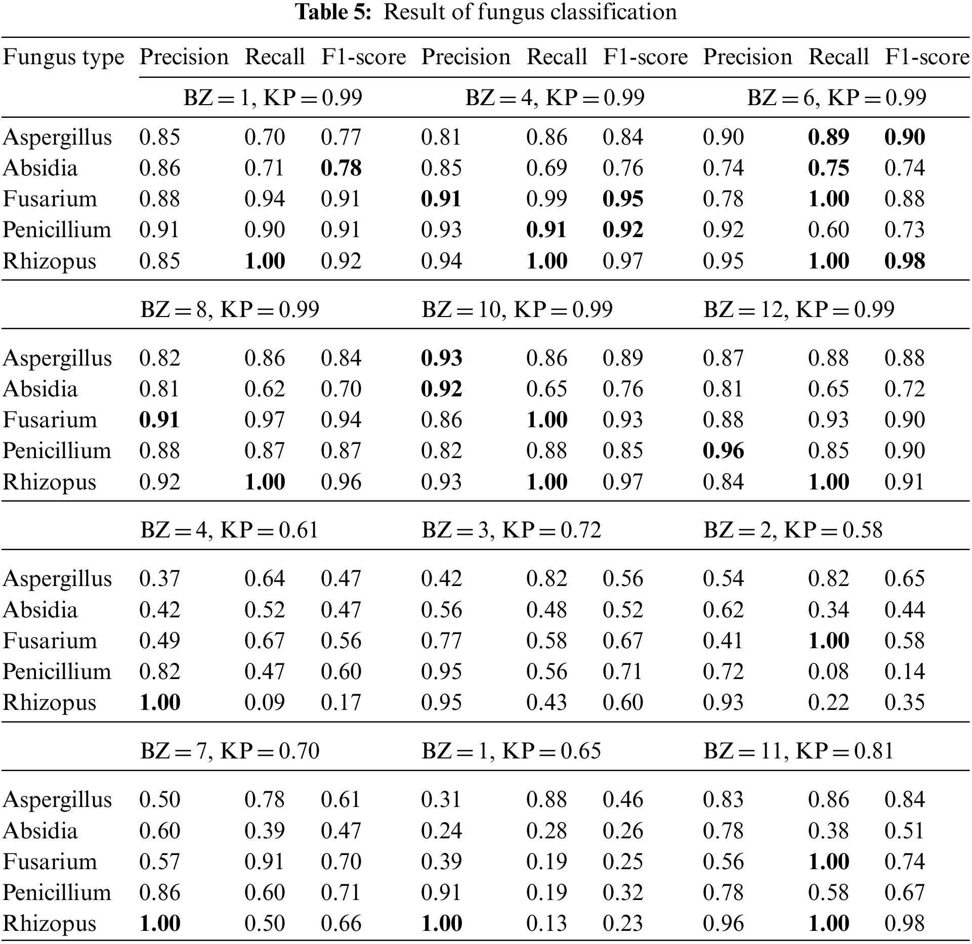
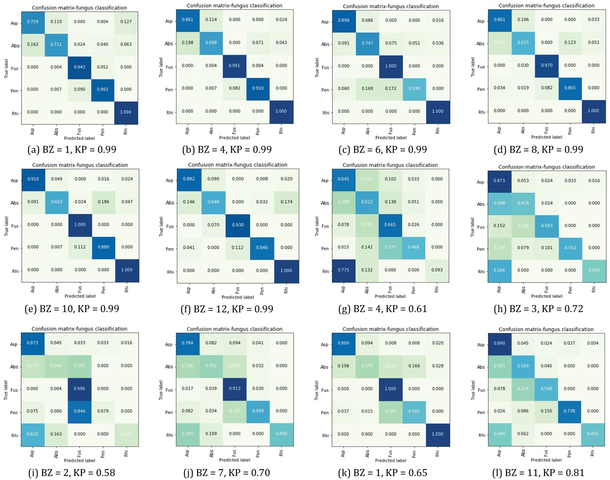
Figure 5: Normalized confusion matrix comparison
The measurement results in Tab. 5 provided the best overall recall efficiency and F1-score when BZ = 6 with KP = 0.99. The recall effectiveness provided 0.89%, 0.75%, 1.00%, and 1.00% to Asp, Fus, Abs, and Rhi. Also, the F1-score significance provided 0.90% and 0.98% to Asp and Rhi. The Recall and F1-score effectiveness, which BZ = 4 with KP = 0.99, provided 0.91% and 0.92%, respectively, for Pen.
According to the classification results by confusion matrix, the test set comparison in the column and row of each class to describe the rate of classification accuracy. The observed color diffusion of the matrix implied classification efficiency. The dark blue area represented an accuracy of 0.800 (80%) to 1.000 (100%). The light blue and green represented predicted data, with errors with an accuracy rate of 0.500 (50%) to 0.790 (79%). The results of Tests 1 and 2 were displayed in Figs. 5a–5c to Fig. 5l.
According to Fig. 5, Asp, Fus, Abs provided the best accuracy efficiency, tested by BZ = 6 and KP = 0.99. Pen had the best efficiency, tested by BZ = 4, 8 with KP = 0.99, conforming to Tab. 5, Rhi had equal efficiency of 1.00 (100%) tested by BZ = 1, 4, 6, 8, 10 and 12 with KP = 0.99.
This research presented the CNN network modified with the 3 different sizes of input filters, i.e., 35 × 35 × 3, 45 × 45 × 3, and 60 × 60 × 3. The advantages also include efficiency enhancement by hyperparameter per round (of practice). On the other hand, small patches of the previous network caused the improper number of patches, failing to gather good data patches for transfer to the next layers [30,35].
According to Test 1, as in Fig. 4a, the test efficiency revealed that the parameter of DB brought high accuracy efficiency to the model, by BZ = 8 with KP = 0.99. The results also revealed the lowest accuracy efficiency, by BZ = 1 with KP = 0.99. The difference between both accuracy efficiency = 2.78%. The enhanced efficiency was also revealed, varying with the sizes of blocks. In this regard, verification revealed the results at the same levels, although BZ = 6 with KP = 0.99 had the efficiency of 97.32% (val_accuracy). The results could be furthered as in Fig. 4b
According to Fig. 4c, the test efficiency revealed that the parameter of DB brought high accuracy efficiency to the model, by BZ = 11 with KP = 0.81. The results also revealed the lowest accuracy efficiency, by BZ = 3 with KP = 0.72. The difference between both accuracy efficiency = 9.94%. According to the results of evaluating accuracy efficiency in Fig. 4d, the best efficiency was found by BZ = 11 with KP = 0.81. The results also revealed the lowest accuracy efficiency, by BZ = 2 with KP = 0.58. The difference between both efficiency = 46.6% (val_accuracy). However, the characteristics of the graphs revealed discontinued learning of the model, resulting in overfitting [33,36]. This problem was analyzed from the test results by BZ = 11 with KP = 0.81 as in Tab. 5. The efficiency of Fus and Rhi = 1.00 (100%), tested by Recall or in Fig. 5l. The test results revealed 1.00 (100%) accuracy of Fus and Rhi.
The fungus database was analyzed for characteristics and data variance through decomposition by PCA in Fig. 6. PC1, PC2, and PC3 were set as the eigenvectors of linear transformation. The key components were displayed in 3D and analyzed by diffusion of color intensity. The relationship of the training set is displayed in Fig. 6a. The relationship of the testing set is displayed in Fig. 6b. Each cluster or species label was written on the axis of its image, i.e., Asp, Abs, Fus, Pen, and Rhi. The data set of training and tests of each species revealed data dispersion without classification.
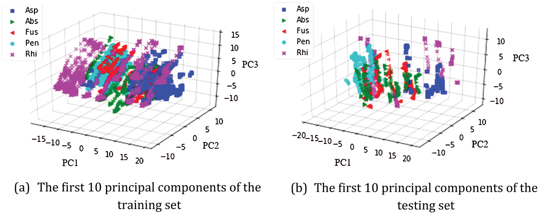
Figure 6: Different color scatters represent different fungus datasets by PCA
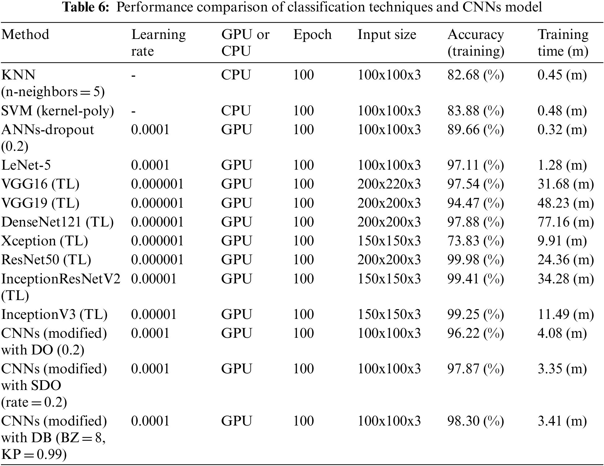
The proposed researcher compared with the previous techniques, shown in Tab. 6, i.e., KNN, SVM, and ANNs. The ANNs contained the number of 2-layer nerve cells, i.e., 30 nodes (Layer 1) and 10 nodes (Layer 2) with dropout (0.2), respectively. The comparison also included dropout (0.2) and SpatialDropout (rate = 0.2), the additional techniques to enhance model efficiency. Furthermore, the suggested technique used more time than KNN (on CPU), SVM (on CPU), and ANNs (on GPU) by 2.96% (n), 2.93% (n), and 3.09% (n). However, its accuracy efficiency was better by 15.62%, 14.42%, and 8.64% because the old methods failed to separate data attributes independently. Even so, the suggested technique contained further steps in terms of extraction, characteristics, and practice. As a result, its efficiency in terms of time was inferior to the old ones. When comparing with LeNet-5 (on GPU), CNNs (modified) with DO (0.2) (on GPU), and CNNs (modified) with SDO (rate = 0.2) (on GPU), the results of the wasted time on training were similar. However, the efficiency of the suggested technique was better by 1.19%, 2.20%, and 0.43% (accuracy) because DB could spread out the net to set areas for extracting data attributes, which could enhance the effectiveness of the model. Also, ResNet50 [15], VGG16 and VGG19 [17], DenseNet121 and Xception [36], InceptionResNetV2 and InceptionV3 [37], are trained with TL method [18] using two layers of fully connected, which each layer consisted of 500 nodes. The results show that the ResNet 50 provides the maximum efficiency at 99.98%, better than the CNNs (modified) with DB (BZ = 8, KP = 0.99) at 1.68%. However, the CNNs (modified) with DB (BZ = 8, KP = 0.99) uses timeless than the ResNet 50 at 7.14 times. It is expressed in Tab. 6.
According to the aims of this research, the modified CNNs models can succeed in identifying each fungus in the data set. It provides reasonable accuracy and timeless computation. However, these results also depend on the training resource and adjusting the parameters in models.
Convolutional Neural Networks (CNNs) have been challenged to image classification with large image datasets applied to biotechnology. This article presents the fungus classification based on efficiently scaled dilation of DropBlock optimization in CNNs. The proposed method can be divided into three parts. Firstly, the preprocessing process is introduced to collect image data from the fives fungus species, including Aspergillus, Absidia, Fusarium, Penicillium, and Rhizopus. Then those image is prepared with image processing technique such as rotation, reflection, images contrast, and Gaussian noise techniques. Secondly, the modified CNNs models are investigated to operate and compared with the previous works by adjusting BlockSize and KeepProp. Finally, the accuracy of the proposed method is measured using Precision, Recall, and F1-score. The experiment results illustrate that the modified CNNs models achieved classify the five fungus species.
Acknowledgement: The authors would like to express sincere gratitude to the Signal Processing Research Laboratory, the Faculty of Engineering, Rajamangala University of Technology Thanyaburi, for insight and expertise.
Funding Statement: This research is supported by the National Research Council of Thailand (NRCT). NRISS No. 906919, 144276, 2589514 (FFB65E0712) and 2589488 (FFB65E0713).
Conflicts of Interest: The authors declare that they have no conflicts of interest to report regarding the present study.
1. X. Simon and P. Loison, “Airborne fungi in workplace atmospheres: Overview of active sampling and offline analysis methods used in 2009–2019,” Encyclopedia of Mycology, vol. 2, pp. 49–58, 2021. [Google Scholar]
2. M. W. Tahir, N. A. Zaidi, A. A. Rao, R. Blank, M. J. Vellekoop et al., “A fungus spores dataset and a convolutional neural network based approach for fungus detection,” IEEE Transactions on NanoBioscience, vol. 17, no. 3, pp. 281–290, 2018. [Google Scholar]
3. J. V. Veasey, P. M. Macedo, J. R. Amorim and R. O. Costa, “The correct nomenclature of zirelí sign in the propaedeutics of pityriasis versicolor,” Anais Brasileiros de Dermatologia, vol. 96, no. 5, pp. 591–594, 2021. [Google Scholar]
4. P. M. Macedo and D. F. S. Freitas, “Superficial infections of the skin and nails,” Encyclopedia of Mycology, vol. 1, pp. 707–718, 2021. [Google Scholar]
5. M. Slaviero, T. P. Vargas, M. V. Bianchi, L. P. Ehlers, A. Spanamberg et al., “Rhizopus microsporus segmental enteritis in a cow,” Medical Mycology Case Reports, vol. 28, pp. 20–22, 2020. [Google Scholar]
6. B. D. Sun, J. Houbraken, J. Frisvad, X. Jiang, A. Chen et al., “New species in aspergillus section usti and an overview of aspergillus section cavernicolarum,” International Journal of Systematic and Evolutionary Microbiology, vol. 70, no. 10, pp. 1–16, 2020. [Google Scholar]
7. J. Cataño and J. Porras, “Adrenal paracoccidioidomycosis,” The American Journal of Tropical Medicine and Hygiene, vol. 103, no. 3, pp. 935–936, 2020. [Google Scholar]
8. R. F. Hector and R. L. Laborin, “Coccidioidomycosis—A fungal disease of the americas,” PLoS Medicine, vol. 2, no. 1, pp. 165–197, 2020. [Google Scholar]
9. C. Smith, A. Tager and B. Mitchell, “The fungus among us: Blastomycosis from spider bites,” Visual Journal of Emergency Medicine, vol. 21, pp. 100825, 2020. [Google Scholar]
10. A. Abdolrasouli and D. A. James, “Aspergillus lung disease,” Encyclopedia of Respiratory Medicine, vol. 4, pp. 40–57, 2022. [Google Scholar]
11. G. N. Tzanetakis, D. Koletsi, A. Tsakris and G. Vrioni, “Prevalence of fungi in primary endodontic infections of a Greek-living population through real-time polymerase chain reaction and matrix-assisted laser desorption/ionization time-of-flight mass spectrometry,” Journal of Endodontics, vol. 48, no. 2, pp. 200–207, 2021. [Google Scholar]
12. M. I. Hussein, D. Jithin, I. J. Rajmohan, A. Sham, E. E. M. A. Saeed et al., “Microwave characterization of hydrophilic and hydrophobic plant pathogenic fungi using open-ended coaxial probe,” IEEE Access, vol. 7, pp. 45841–45849, 2019. [Google Scholar]
13. L. Liu, Y. Yuan, J. Zhang, H. Lei, Q. Wang et al., “Automatic identification of fungi under complex microscopic fecal images,” Journal of Biomedical Optics, vol. 20, no. 7, pp. 76004, 2015. [Google Scholar]
14. M. W. Tahir, N. A. Zaidi, R. Blank, P. P. Vinayaka, M. J. Vellekoop et al., “Fungus detection through optical sensor system using two different kinds of feature vectors for the classification,” IEEE Sensors Journal, vol. 17, no. 16, pp. 5341–5349, 2017. [Google Scholar]
15. C. Domínguez, J. Heras, E. Mata and V. Pascual, “DecoFungi: A web application for automatic characterisation of dye decolorisation in fungal strains,” BMC Bioinformatics, vol. 19, no. 66, pp. 1–4, 2018. [Google Scholar]
16. R. Hao, X. Wang, J. Zhang, J. Liu, X. Du et al., “Automatic detection of fungi in microscopic leucorrhea images based on convolutional neural network and morphological method,” in Information Technology, Networking, Electronic and Automation Control Conf. (ITNEC), Chengdu, China, pp. 2491–2494, 2019. [Google Scholar]
17. X. Du, L. Liu, X. Wang, G. Ni and J. Zhang, “Intelligent identification of microscopic visible components in leucorrhea routine,” in Information Technology, Networking, Electronic and Automation Control Conf. (ITNEC), Chengdu, China, pp. 2344–2349, 2019. [Google Scholar]
18. M. A. Santoyo, C. Domínguez, J. Heras, E. Mata, V. Pascual et al., “Automatic characterisation of dye decolourisation in fungal strains using expert, traditional, and deep features,” Soft Computing, vol. 23, no. 23, pp. 12799–12812, 2019. [Google Scholar]
19. Y. Zhou, Y. Feng and H. Zhang, “Human fungal infection image classification based on convolutional neural network,” Image and Graphics Technologies and Applications, vol. 1043, pp. 1–12, 2019. [Google Scholar]
20. B. Zeliński, A. Sroka, D. Rymarczyk, A. Piekarczyk and M. B. Włoch, “Deep learning approach to description and classification of fungi microscopic images,” PLoS ONE, vol. 15, no. 6, pp. 1–16, 2019. [Google Scholar]
21. A. Prommakhot and J. Srinonchat, “Exploiting convolutional neural network for automatic fungus detection in microscope images,” in International Electrical Engineering Congress (iEECON), Chiang Mai, Thailand, pp. 1–4, 2020. [Google Scholar]
22. M. Fan, T. Chakraborti, E. I. Chang, Y. Xu and J. Rittscher, “Fine-grained multi-instance classification in microscopy through deep attention,” in IEEE Int. Symp. on Biomedical Imaging (ISBI), Iowa, USA, pp. 169–173, 2020. [Google Scholar]
23. J. P. Latgé and G. Chamilos, “Aspergillus fumigatus and aspergillosis in 2019,” Clinical Microbiology Reviews, vol. 33, no. 1, pp. e00140–18, 2019. [Google Scholar]
24. T. K. Zong, H. Zhao, X. L. Liu, L. Y. Ren, C. L. Zhao et al., “Taxonomy and phylogeny of four new species in absidia (cunninghamellaceae, mucorales) from China,” Frontiers in Microbiology, vol. 12, pp. 2181, 2021. [Google Scholar]
25. H. Younesi, E. Bazgir, M. Darvishnia, and K. Chehri, “Selection and control efficiency of trichoderma isolates against fusarium oxysporum f. sp. ciceris in Iran,” Physiological and Molecular Plant Pathology, vol. 116, pp. 101731, 2021. [Google Scholar]
26. A. Mincuzzi, A. Ippolito, C. Montemurro, and S. M. Sanzani, “Characterization of penicillium s.s. and aspergillus sect. nigri causing postharvest rots of pomegranate fruit in southern Italy,” International Journal of Food Microbiology, vol. 314, no. 6, pp. 108389, 2020. [Google Scholar]
27. T. C. Pham, A. Doucet, C. M. Luong, C. T. Tran and V. D. Hoang, “Improving skin-disease classification based on customized loss function combined with balanced mini-batch logic and real-time image augmentation,” IEEE Access, vol. 8, pp. 150725–150737, 2020. [Google Scholar]
28. V. Anand, S. Gupta, D. Koundal, S. Mahajan, A. K. Pandit et al., “Deep learning based automated diagnosis of skin diseases using dermoscopy,” CMC-Tech Science Press, vol. 71, no. 2, pp. 3145–3160, 2022. [Google Scholar]
29. S. Elghamrawy, A. E. Hassanien and V. Snasel, “Optimized deep learning-inspired model for the diagnosis and prediction of COVID-19,” CMC-Tech Science Press, vol. 67, no. 2, pp. 2353–2371, 2021. [Google Scholar]
30. F. Yang, M. Poostchi, H. Yu, Z. Zhou, K. Silamut et al., “Deep learning for smartphone-based malaria parasite detection in thick blood smears,” IEEE Journal of Biomedical and Health Informatics, vol. 24, no. 5, pp. 1427–1438, 2020. [Google Scholar]
31. M. Alrahhal, Y. Bazi, R. M. Jomaa, M. Zuair and N. Alajlan, “Deep learning approach for COVID-19 detection in computed tomography images,” CMC-Tech Science Press, vol. 67, no. 2, pp. 2093–2110, 2021. [Google Scholar]
32. N. Srivastava, G. Hinton, A. Krizhevsky, I. Sutskever and R. Salakhutdinov, “Dropout: A simple way to prevent neural networks from overfitting,” Journal of Machine Learning Research, vol. 15, no. 56, pp. 1929–1958, 2014. [Google Scholar]
33. J. Tompson, R. Goroshin, A. Jain, Y. LeCun and C. Bregler, “Efficient object localization using convolutional networks,” in IEEE Conf. on Computer Vision and Pattern Recognition (CVPR), Boston, MA, USA, pp. 648–656, 2015. [Google Scholar]
34. G. Ghiasi, T. Y. Lin and Q. V. Le, “Dropblock: A regularization method for convolutional networks,” in Annual Conference on Neural Information Processing Systems, Montreal, Canada, pp. 10750–10760, 2018. [Google Scholar]
35. L. Qian, L. Hu, L. Zhao, T. Wang and R. Jiang, “Sequence-dropout block for reducing overfitting problem in image classification,” IEEE Access, vol. 8, pp. 62830–62840, 2020. [Google Scholar]
36. P. Pisantanaroj, P. Tanpisuth, P. Sinchavanwat, S. Phasuk and P. Phienphanich, “Automated firearm classification from bullet markings using deep learning,” IEEE Access, vol. 8, pp. 78236–78251, 2020. [Google Scholar]
37. A. Rao, T. Nguyen, M. Palaniswami and T. Ngo, “Bird species classification using transfer learning with multistage training,” Structural Health Monitoring, vol. 20, pp. 1–19, 2020. [Google Scholar]
 | This work is licensed under a Creative Commons Attribution 4.0 International License, which permits unrestricted use, distribution, and reproduction in any medium, provided the original work is properly cited. |