Computers, Materials & Continua DOI:10.32604/cmc.2022.024490
Article

Optimal Bidirectional LSTM for Modulation Signal Classification in Communication Systems

Manar Ahmed Hamza1,*, Siwar Ben Haj Hassine2, Souad Larabi-Marie-Sainte3, Mohamed K. Nour4, Fahd N. Al-Wesabi5,6, Abdelwahed Motwakel1, Anwer Mustafa Hilal1 and Mesfer Al Duhayyim7

1Department of Computer and Self Development, Preparatory Year Deanship, Prince Sattam bin Abdulaziz University, AlKharj, Saudi Arabia
2Department of Computer Science, College of Science and Arts, King Khalid University, Mahayil Asir, Saudi Arabia
3Department of Computer Science, College of Computer and Information Sciences, Prince Sultan University, Saudi Arabia
4Department of Computer Science, College of Computing and Information System, Umm Al-Qura University,Saudi Arabia
5Department of Computer Science, College of Science & Art at Mahayil, King Khalid University, Saudi Arabia
6Faculty of Computer and IT, Sana'a University, Sana'a, Yemen
7Department of Natural and Applied Sciences, College of Community-Aflaj, Prince Sattam bin Abdulaziz University, Saudi Arabia
*Corresponding Author: Manar Ahmed Hamza. Email: ma.hamza@psau.edu.sa
Received: 19 October 2021; Accepted: 20 December 2021

Abstract: Modulation signal classification in communication systems can be considered a pattern recognition problem. Earlier works have focused on several feature extraction approaches such as fractal feature, signal constellation reconstruction, etc. The recent advent of deep learning (DL) models makes it possible to proficiently classify the modulation signals. In this view, this study designs a chaotic oppositional satin bowerbird optimization (COSBO) with bidirectional long term memory (BiLSTM) model for modulation signal classification in communication systems. The proposed COSBO-BiLSTM technique aims to classify the different kinds of digitally modulated signals. In addition, the fractal feature extraction process takes place by the use of Sevcik Fractal Dimension (SFD) approach. Moreover, the modulation signal classification process takes place using BiLSTM with fully convolutional network (BiLSTM-FCN). Furthermore, the optimal hyperparameter adjustment of the BiLSTM-FCN technique takes place by the use of COSBO algorithm. In order to ensure the enhanced classification performance of the COSBO-BiLSTM model, a wide range of simulations were carried out. The experimental results highlighted that the COSBO-BiLSTM technique has accomplished improved performance over the existing techniques.

Keywords: Complex systems; communication system; signal processing; modulation signals; classification; artificial intelligence; deep learning; parameter tuning

1  Introduction

Currently, the growth of wireless communication technologies demonstrates the trends of rapid development, and gradually the conventional ground communication technique cannot meet peoples’ day to day requirements, hence scholars and experts increasingly focus on the study of satellite communication technology. Now, wireless communication technology was employed to peoples’ livelihood and national defence, however, data intervention and emerging challenges have become increasingly prominent [1,2]. In the limited space, the density of wireless signals has been improved dramatically, hence, to extend the bandwidth of wireless signals, we have to exploit distinct modulation systems for signal modulation. The detection technique of modulation signal is amongst demodulating and receiving [3]. Afterward getting the wireless signal, the process of extracting the modulation signal from the noisy signal could provide a basis for the signal data extraction of the signal, parameter estimation, and succeeding demodulation.

As a traditional pattern recognition problem, the modulation detection of transmission signals has several application values and important research prospects [4]. In the military fields, it is a precondition to implement jamming and transmission reconnaissance. When the signal modulation of the enemy's transmission scheme has been described, the enemy's signal could be demodulated and data transmission could be attained. In the civil fields, signal modulation detection could be utilized for interference identification, signal confirmation, spectrum monitoring, and spectrum management [5]. Thus, a reliable and secure feature extraction technique is required for efficiently recognizing the distinct signal modulations in a difficult environment. Generally, Modulation pattern recognition employs decision-making methods and statistical pattern recognition methods. Now, many applications are statistical pattern recognition method that is separated to 2 stages: classifier design and feature extraction [6]. Good features are a key element to enhance classification performance. Recently, authors have presented different approaches to extract feature parameters like fractal features, signal constellation reconstruction, instantaneous features, and so on. Since other major factors of signal pattern recognition, classifier straightforwardly determines the classification accuracy.

Deep learning (DL) algorithm could extract the fundamental feature and incorporate them to attain the high-level features [7]. Afterward, including attribute classes of feature, the feature distribution characteristic of the target objects could be examined. Furthermore, the DL method has a stronger capacity for fitting the features of information. Lately, several researches have illustrated that neural network/machine learning could be employed to signal pattern recognition/signal feature extraction, however, the realtime application would be influenced by the changes of signal to noise ratio (SNR) [8]. The detection of modulation signals through DL method has higher strength, and also the recognition kinds are very exhaustive. However, in realtime applications, it would be complex to realize due to the difficulty of the model [9]. Thus, it is very important for constructing a modulation signal pattern recognition method with large dynamic and good generalization SNR. But, it is a major problem to manually detect the recognition method, the modulation system of the classifiers in the modulation signal efficiently, and the characteristics parameter and employ it to the detection of the modulation signal patterns.

This study designs a chaotic oppositional satin bowerbird optimization (COSBO) with bidirectional long term memory (BiLSTM) model, called COSBO-BiLSTM for modulation signal classification in communication systems. The proposed COSBO-BiLSTM technique encompasses Sevcik Fractal Dimension (SFD) approach for feature extraction. In addition, the modulation signal classification process takes place using BiLSTM with fully convolutional network (BiLSTM-FCN). Finally, the optimal hyperparameter adjustment of the BiLSTM-FCN technique is performed using the COSBO algorithm. For examining the better outcomes of the COSBO-BiLSTM technique, a detailed experimental analysis takes place and the results are inspected under several aspects.

2  Related Works

Xu et al. [10] examine the appropriate framework of DL model in the field of transmission signal recognition. According to the framework analyses of the convolutional neural network (CNN), the authors utilized actual signal information and attained well-suited detection performance of modulation classification than many illustrative structures. The authors declare that the deep network framework isn't appropriate for signal recognition because of its distinct characteristics. Zha et al. [11] investigate algorithms for modulation classification and multi signal detection that is important in several transmission schemes. In this study, a DL architecture for modulation recognition and multi-signals detection has been presented. In comparison with present approaches, the start-stop time, signal modulation format, and centre frequency could be attained from the presented system.

Wang et al. [12] create a multi-layer hybrid machine learning (ML) network for the classification of 7 kinds of signals in distinct modulations. The authors extract the signal modulation feature exploit a group of methods like discrete Fourier transform, instantaneous autocorrelation, and time-frequency analysis, and achieve automated modulation classification with Naïve Bayes (NB) and SVM in a hybrid method. The parameter in the network for classification are defined manually in the training method. Peng et al. [13] examine the usage of the DL in modulation classification, i.e., a primary task in various communication methods. The DL is based on a huge number of information and, for applications and, research this could be easily accessible in communication schemes. Different from ML, the DL has the benefit of not needing automatic feature selection that considerably reduces the task difficulty in modulation classification. In this work, the authors employ two CNN-based DL methods such as GoogLeNet and AlexNet.

Wang et al. [14] discuss the modulation recognition process, i.e., a significant part of transmission system through the DL approach. Unlike the traditional ML approaches which need feature extraction, the DL approach doesn't need feature extraction and attains further impacts when compared to traditional ML method. Ali et al. [15] investigate the applications of deep neural network (DNN) to the automated modulation classification in adaptive white Gaussian noise (AWGN) and flat-fading channels. The 3 training inputs have been utilized; mostly 1) the higher order cumulant of received samples 2) In-phase and quadrature (I-Q) constellation point, and 3) the centroid of constellation point using the fuzzy C-means approach to I-Q model. The unsupervised learning from these datasets has been made by the sparse autoencoder and supervised softmax classifiers have been applied for the classification.

Güner et al. [16], proposed a novel automatic modulation classification (AMC) system with extreme learning machine (ELM) as classifiers that contain a better generalization performance and fast-learning method when compared to traditional ML approaches. Also, the researchers examined the stability of the presented AMC system which gets influenced by variations in the value of the frequency, phase offset, and roll-off factor. Wu et al. [17] presented an improved deep neural framework to implement radio signal identification task, i.e., a significant facet of creating the spectrum sensing ability needed by software determined radio. The modules in the presented network combine the advantage of ResNet and, Inception network that contains larger receptive field and fast convergence rate. The presented system is demonstrated to have outstanding performances for modulation classification.

Zhou et al. [18], proposed a strong AMC approach with CNN. Altogether, fifteen distinct modulation kinds are taken into account. The presented model could categorize the received signal directly without feature extraction, and it could manually learn features from the received signal. The feature learned by the CNNs is analyzed and presented. The strong feature of the received signal in a certain SNR range is investigated. Lin et al. [19] focus on DL which aims utilizing it to resolve transmission problems. The authors proposed a novel data conversion method for gaining an improved classification performance of transmission signal modulation. This study would demonstrate that the novel approach would bring substantial growth in signal modulation classification performance.

3  The Proposed Method

In this study, a new COSBO-BiLSTM technique is derived to classify the different kinds of digitally modulated signals in communication systems. The proposed COSBO-BiLSTM technique comprises three stages of operations such as SFD based feature extraction, BiLSTM-FCN based modulation signal classification, and COSBO based hyperparameter optimization. The utilization of COSBO algorithm helps to considerately improve the overall classification efficiency of the BiLSTM-FCN technique. Fig. 1 illustrates the overall working process of COSBO-BiLSTM model. The detailed working of these modules is provided in the following sections.

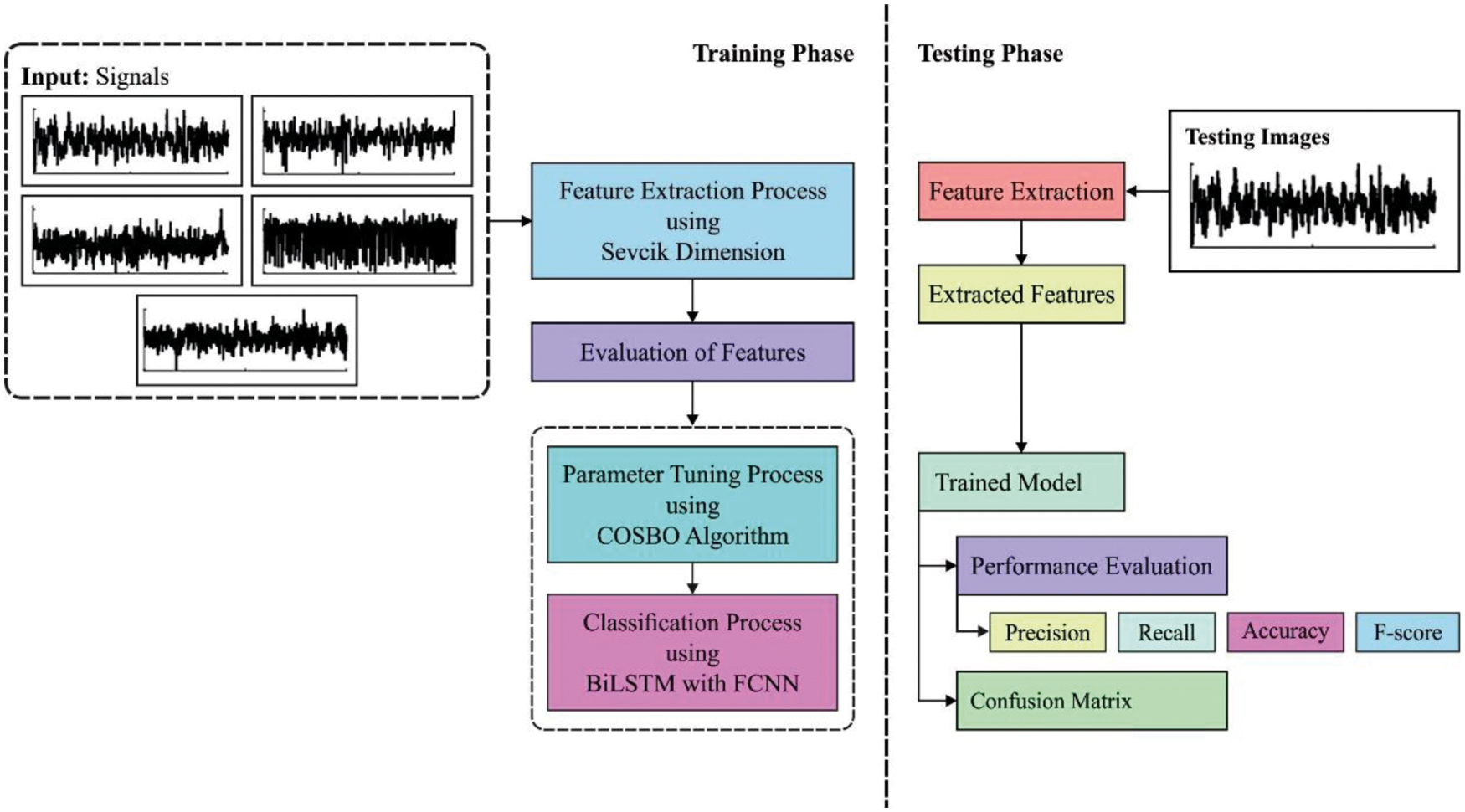
Figure 1: Overall process of COSBO-BiLSTM model

3.1 Feature Extraction Using SFD Technique

In this phase, the fractal feature from the transmission signal is extracted by the SFD method. The self-similar dimension is complex to employ objects which are not severely self-similar, and the box dimension can be used to overcome this challenge. In the metric space (X,d),A has belonged to M non-empty emergency cluster of X. For a box utilizing side length of ε, the minimum value N(A,ε) of box required to cover A can be expressed as follows:

N(A,ε)={M:A⊂∑i=1M⁡N(xi,ε)}(1)

where x1,x2,…xM signify dissimilar points of X. Whereas ε approaching 0, the box dimension can be shown in Eq. (2)

Db=limε→0⁡InN(A,ε)In(1/ε)(2)

As above-mentioned, assume the signal consists of a series of points (xi,yi), the length of signals is N. Initially, standardize the signal [20]:

xi∗=xi−xxmax−x,yi∗=yi−ymax−y(3)

xmin,ymin characterizes the minimum values between xj,yj.xmax,ymax denotes the maximum values between xj,yj. Then, the Sevcik fractal dimension D is evaluated by:

D=1+ln(L)+ln(2)ln[2×(N−1)](4)

where L denotes the length of waveform, as:

L=∑i=0N−2⁡(yi+1∗−yi∗)2+(xi+1∗−xi∗)2(5)

3.2 Modulation Signal Classification Using BiLSTM-FCN Technique

At this stage, the features are fed into the BiLSTM-FCM model to categorize the modulation signals. Hochreiter and Schmidhuber have been established the long short term memory (LSTM) primarily for overcoming the vanishing gradient issue. The LSTM has been different from recurrent neural network (RNN) which is similar kind of input and output. But, in difference to RNN, LSTM is an input, forget, and output gate. Hence, it has controls that kept and forgotten. The LSTM holds data in the past, but RNN could not. Put properly, computation in the LSTM technique takes in keeping with the succeeding computation that is applied at all the time steps. These computations give the complete technique to a new LSTM with forget gate:

g(z)=tanh⁡(Wgxx(z)+Wghh(z−1)+bg)(6)

i(z)=σ(Wixx(z)+Wihh(z−1)+bi)(7)

f(z)=σ(Wfxx(z)+Wfhh(z−1)+bf)(8)

o(z)=σ(Woxx(z)+Wohh(z−1)+bo)(9)

s(z)=g(z)⊙i(i)+s(z−1)⊙f(z)(10)

h(z)=tanh(s(z))⊙o(z)(11)

where x(z) refers the input layer at present time step z, h(z) signifies the value of hidden layer of LSTM, but h(z−1) indicates the outcome values with all memory cells from the hidden layer at earlier times. The σ stands for the sigmoid function, ⊙ and tanh demonstrates the element-wise multiplication and hyperbolic tangent function correspondingly. The Bi-LSTM procedures order data from all forward as well as backward directions with 2 distinct hidden layers for capturing previous and future data correspondingly; afterward, the 2 hidden states have been concatenated for producing last output.

CNN is the image processing technique, which have the capability for yielding hierarchies of features. The fully convolutional networks (FCNs) have been generally implemented from the temporal domain and ended up that helps to control the temporal dimensional in lacking some immense data pre-processed and feature engineering. During the presented techniques, it can be utilized FCN as feature extractor from the primary branch of both techniques [21]. For univariate time series classification (TSC), FCN has been explained as:

z=w⊛x+b(12)

a=BN(z)(13)

y=ReLU(a)(14)

where w, x, and b indicates the tensor, input vector, and bias vector at output vector z correspondingly, and ⊛ refers the convolutional operator. The FCN framework has 3 convolution 1D kernels (8, 5, and 3). All the blocks are succeeded by batch normalization (BN) and rectified linear unit (ReLU) activation layers. Next to the convolution blocks, the features are fed into the global average pooling layers, and the last layer will be the softmax layer.

It can be augmented BiLSTM and fuzzy c-means (FCM) for proposing end-to-end hybrid techniques as BiLSTM regards combination of forward as well as backward dependencies from the time series data. But the FCN is the capability for taking hierarchies of features, the consumption of attention process permits the network for focusing on the ardently salient part of time series data. The presented technique framework has 2 branches, FCN, and BiLSTM. An initial branch has been the convolution part of technique utilized as feature extractors; this block is 3 convolution 1D kernels with sizes (kernel sizes of 8, 5, and 3) without striding. All the layers and then BN for improving the speed, efficiency, and consistency of networks and ReLU activation layer for fixing the vanishing gradient problem from the DNN, and generate the last network by stacking 3 convolutional blocks with filter sizes 128, 256, and 128 from all the blocks. Afterward the convolutional blocks, the features have been feed as to global average pooling layer. The second branch contains BiLSTM block. The BiLSTM trained 2 LSTMs in any one place that is access long-range context from combined of forward as well as backward ways from the time series data. The BiLSTM block receives a changed time series then dimensional shuffle layer also transfers the temporal dimensional of time series, then dropout, for avoiding over-fit, and at last, the outcome of 2 branches are concatenated and feed into SoftMax classifiers.

3.3 Hyperparameter Tuning Using COSBO Algorithm

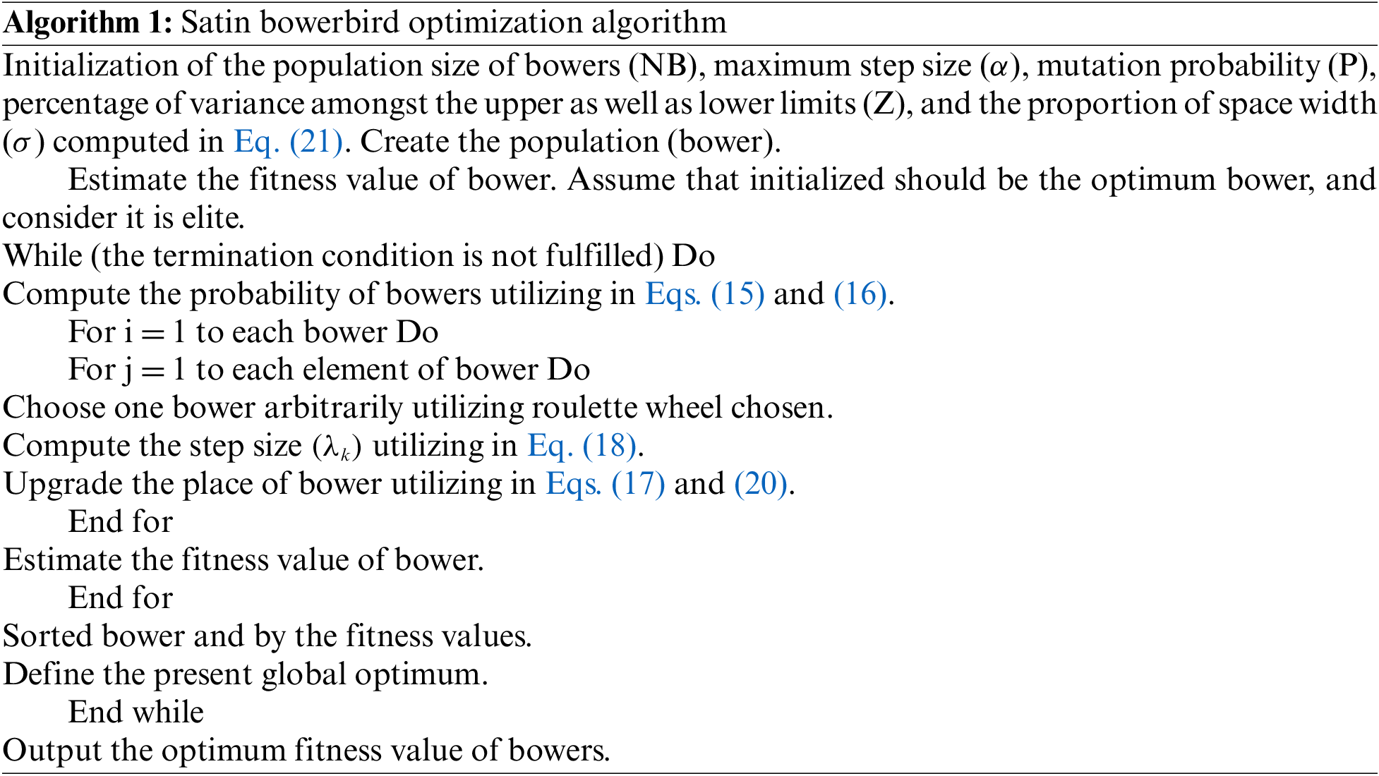
For optimally adjusting the hyperparameters of the BiLSTM-FCN model, the COSBO algorithm is applied. The SBO technique has been population-based approach that evaluates the global optimal to provide optimize issues [22]. It can be population dependent upon a stochastic optimize technique and is extremely robust, straightforward, and effectual. In 2 important models that represent the SBO technique:

1.    How to compute the probabilities of all the population members.

2.    How to define a novel modifies from someplace.

3.    How to progress mutation.

The succeeding sub-sections more determine these techniques. The generation of arbitrary bowers procedure begins with generating a population of arbitrary uniform distributions, with the regard as combined of the lower as well as upper limit parameters. Followed by, all the positions are determined as dimension vectors of parameters that can be optimized. The probabilities of such determine the attractiveness of bower. The female satin bower bird chooses the bower (nest) dependent upon their probabilities and is capable of calculating the probabilities of all the population members in Eqs. (15) and (16) under.

Probi=fiti∑n=1NB⁡fitn(15)

fiti={11+f(xi),f(xi)≥01+|f(xi)|,f(xi)<0(16)

where NB refers the population size of bower, fiti signifies the fitness value of ith solution, and f(xi) represents the fitness value of ith bower. Fig. 2 depicts the process flow of SBO technique.

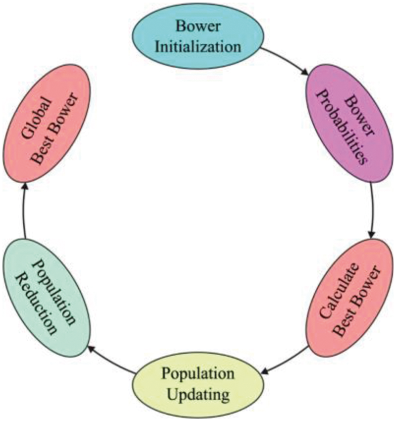
Figure 2: Process of SBO technique

The SBO technique utilizes the model of elitism that defines the place of the optimum bowers, so permitting the optimum solutions that are maintained at all the stages of optimized model. The SBO technique replicates the process of birds constructing nests with its natural instinct. During the mating season, the male satin bower bird utilizes his natural instinct for creating and decorating his bower, in an effort for attracting female birds. It can be inferred that male bowers depend on their experience for influencing their creative decision from generating their bowers; so, further experience bird is generating further attractive bower (enhancing their fitness) than minimum experienced birds [23]. During this case, an optimum-built bower (optimal place) has been projected as elite iterations. As the elite place is the maximum fitness, it can be capable of influencing another place. The variations of all novel bowers demonstrating a novel place defined as the place of an optimum fit bower (place) have been computed based on Eq. (17).

xiknew=xikold+λk((xjk+xelite,k2)−xikold)(17)

where xi refers the ith solution vectors (bowers), xj defines as the destination solution amongst every solution from the present iterations, j signifies the computed as the roulette wheel process, and xik indicates the kth member of dimensional. xelite denotes the elite place (an optimum fitness value from the present iteration). In Eq. (4), λk demonstrates the attraction power of goal bowers demonstrated at intervals of λk∈(0,1), where α implies the maximal step size (constant); and pj stands for the probabilities attained in Eq. (15) utilizing the aim bower at intervals of pj∈(0,1).

λk=α1+pj(18)

During the mutation process that takes place at the end of all iterations of SBO, arbitrary modifies have been implemented to xik with particular probabilities. The normal distribution (N) in the mutation function has been utilized with an average of xikold, and the variance of σ2, as realized in Eqs. (19)–(21)

xiknew∼N(xikold,σ2)(19)

N(xikold,σ2)=xikold+(σ∗N(0,1))(20)

σ=Z∗(varmax−varmin)(21)

where σ implies the proportion of space width and varmin and varmax signifies the lower as well as upper bounds allocated to the variables. The value of Z parameter is the percent of variance amongst lower as well as upper limits that have variables. In the final stage of all iterations, the recently generated populations and the primary populations have been estimated, and every population has been joined and sorted by its fitness value. A novel population is then made based on the earlier well-defined number, but others are rejected. The fundamental steps of SBO are drawn in Algorithm 1.

But, the SBO approach provides likely outcome for the optimization problem, its lower convergence speed in many challenges makes a weaker solution or even an inappropriate solution. In this work, 2 methods are used to decrease these problems as possible. The initial term is to utilize a Quasi-oppositional learning method. In order to understand the concept of this model, first the authors determine the fundamental oppositional learning method. The oppositional learning technique is utilized to modify the premature convergence problems by comparing all individuals of the population with its opposite values and for selecting the better one as an appropriate candidate [24]. This method is implemented by considering a candidate x as a real number in the search space with d-dimensional in the interval [α,β]. In this scenario, the opposite method for an individual x is attained by:

x~ι=αi+βi−xi(22)

i=1,2,…,D(23)

Based on the description of the opposite method, the quasi-opposite number can be attained by:

x^i=rand(αi+βi2,x~ι)(24)

The above mentioned approach is utilized for the population generation. Next, it is applied to the chaotic method. According to the chaos concept, the real nature of system is nonlinear and complicated, as well as some mechanism seems random, however, the authors have an equated pseudo random nature. This method is used for accelerating the quasi-opposite through pseudo-random values rather than random values in all the iterations. The current research employs the logistic map as a chaotic method for modifying the quasi-opposite method. The logistic map can be expressed by:

δo,nq+1=4δo,nq(1−δo,nq)(25)

whereas o defines the value of the system generator, n represent the population count, q indicates the iteration count, δn signifies the chaotic method in iteration n i.e., in the range of zero and one. As abovementioned, the novel population in the upcoming iteration would be generated as follows:

x^nq+1=δo,nq×x^nq(26)

4  Result and Discussion

The performance validation of the COSBO-BiLSTM technique takes place under various aspects. Fig. 3 shows the SFD features of different communication signals. The figure has shown that the fractal features are investigated under varying SNR levels. It is noticed that the fractal features get reduced with an increase in SNR levels. The confusion matrix generated by the BiLSTM-FCN model under run-1 is portrayed in Fig. 4. The figure reported that the BiLSTM-FCN model has identified 191 instances into 2ASK, 188 instances into 4ASK 200 instances into 2FSK, 193 instances into 4FSK, 186 instances into 8FSK, 200 instances into BPSK, 198 instances into 16QAM, and 189 instances into 32QAM.

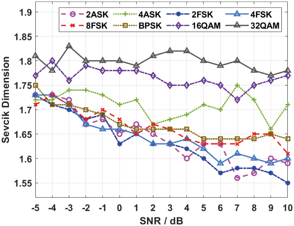
Figure 3: Fractal features of various communication signals

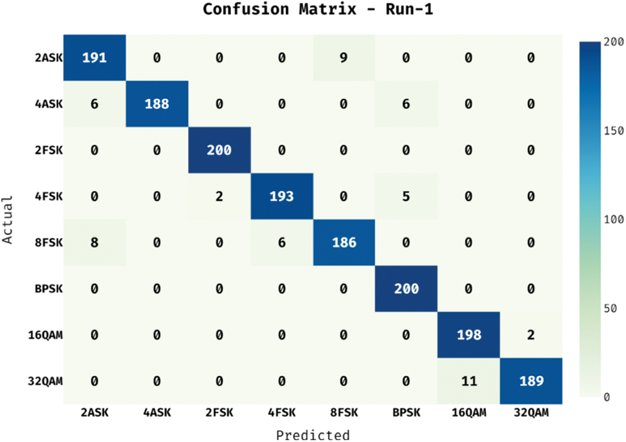
Figure 4: Confusion matrix of BiLSTM-FCN model under test run-1

The confusion matrix generated by the BiLSTM-FCN approach under run-2 is showed in Fig. 5. The figure reported that the BiLSTM-FCN approach has identified 190 instances into 2ASK, 190 instances into 4ASKm, 200 instances into 2FSK, 193 instances into 4FSK, 184 instances into 8FSK, 200 instances into BPSK, 197 instances into 16QAM, and 188 instances into 32QAM. Tab. 1 portrays the overall modulation signal classification performance of the BiLSTM-FCN model under two test runs. The experimental values stated that the BiLSTM-FCN model has appropriately classified the modulation signals effectively under two test runs. For instance, with run-1, the BiLSTM-FCN model has proficiently classified the modulation signals with the average PREN, RECL, ACCY, and FSCORE of 0.9663, 0.9656, 0.9914, and 0.9656. Moreover, under run-2, the BiLSTM-FCN model has proficiently classified the modulation signals with the average PREN, RECL, ACCY, and FSCORE of 0.9643, 0.9637, 0.9909, and 0.9637.

Figure 5: Confusion matrix of BiLSTM-FCN model under test run-2

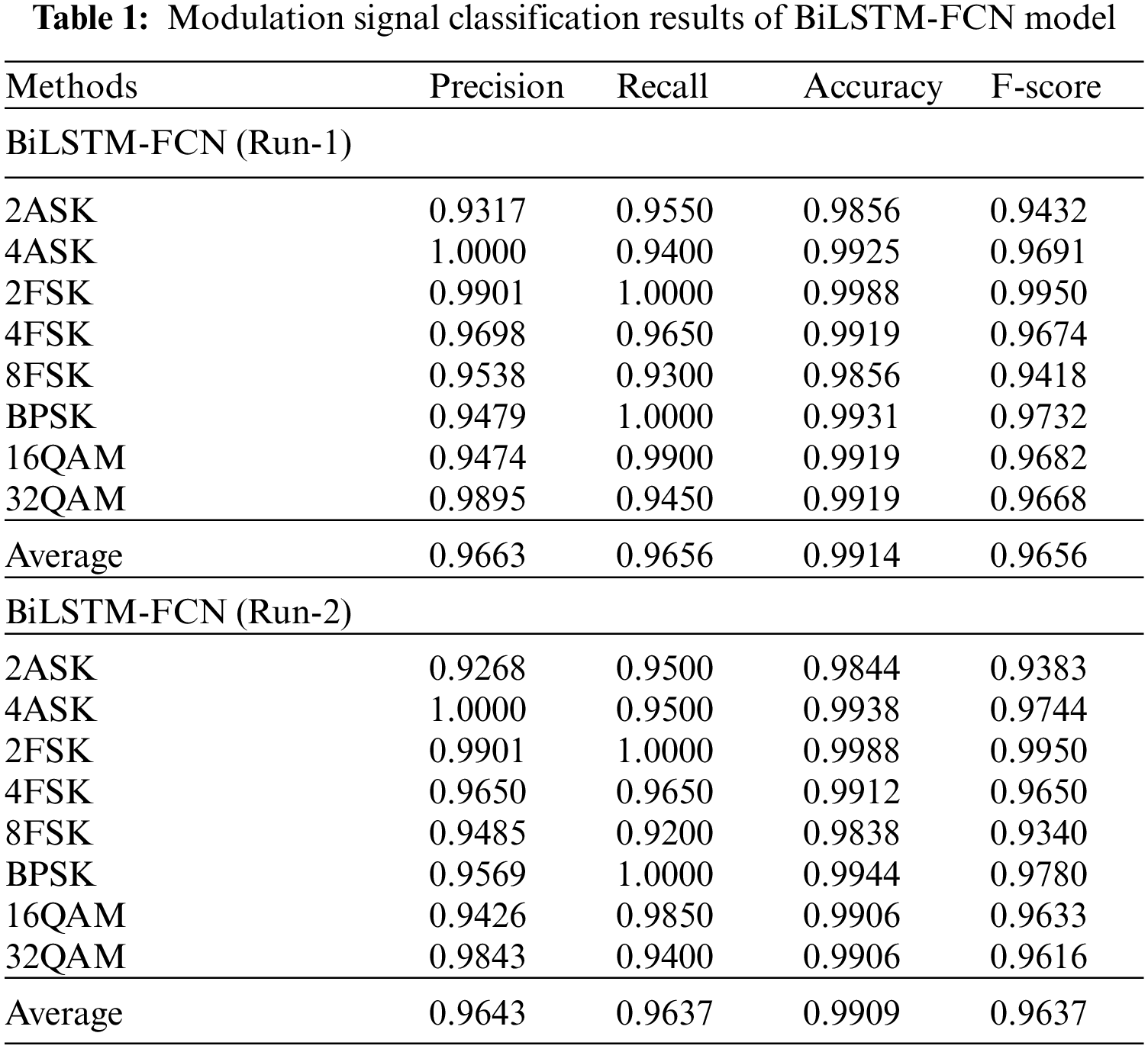
The confusion matrix generated by the COSBO-BiLSTM technique under run-1 is shown in Fig. 6. The figure reported that the COSBO-BiLSTM method has identified 197 instances into 2ASK, 197 instances into 4ASKm, 200 instances into 2FSK, 200 instances into 4FSK, 195 instances into 8FSK, 200 instances into BPSK, 200 instances into 16QAM, and 196 instances into 32QAM as shown in Fig. 7.

Figure 6: Confusion matrix of COSBO-BiLSTM model under test run-1

Figure 7: Confusion matrix of COSBO-BiLSTM model under test run-2

Tab. 2 shows the overall modulation signal classification accuracy of the COSBO-BiLSTM methodology under two test runs. The experimental values stated that the COSBO-BiLSTM system has appropriately classified the modulation signals efficiently under two test runs. For instance, with run-1, the COSBO-BiLSTM approach has proficiently classified the modulation signals with the average PREN, RECL, ACCY, and FSCORE of 0.9907, 0.9906, 0.9977, and 0.9906. Furthermore, under run-2, the COSBO-BiLSTM model has proficiently classified the modulation signals with the average PREN, RECL, ACCY, and FSCORE of 0.9925, 0.9925, 0.9981, and 0.9925.

The overall classification results analysis of the BiLSTM-FCN model under two execution runs is shown in Fig. 8. The figure reported that the BiLSTM-FCN model has classified the modulation signals under run-1 into average PREN, RECL, ACCY, and FSCORE of 0.9663, 0.9656, 0.9914, and 0.9656. At the same time, under run-2, the BiLSTM-FCN model has proficiently identified the modulation signals with the average PREN, RECL, ACCY, and FSCORE of 0.9643, 0.9637, 0.9909, and 0.9637.

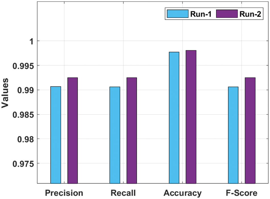
Figure 8: Overall analysis of BiLSTM-FCN model with distinct measures

The overall classification outcomes analysis of the COSBO-BiLSTM method in 2 execution runs is shown in Fig. 9. The figure reported that the COSBO-BiLSTM approach has classified the modulation signals under run-1 into average PREN, RECL, ACCY, and FSCORE of 0.9907, 0.9906, 0.9977, and 0.9906. Simultaneously, under run-2, the COSBO-BiLSTM technique has proficiently identified the modulation signals with the average PREN, RECL, ACCY, and FSCORE of 0.9925, 0.9925, 0.9981, and 0.9925.

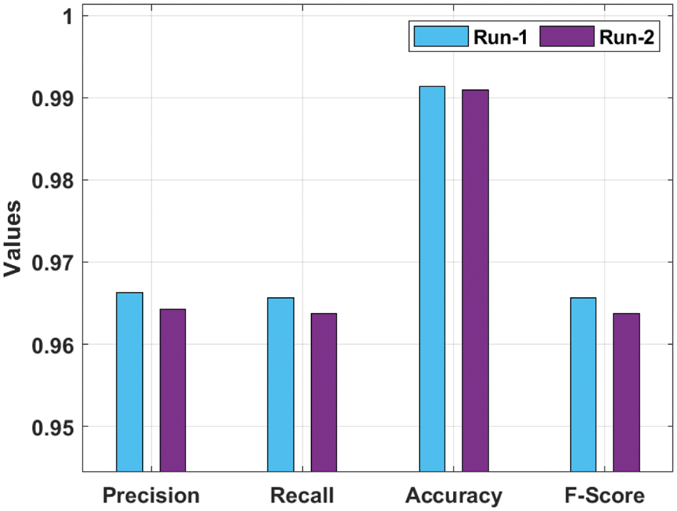
Figure 9: Overall analysis of COSBO-BiLSTM model with distinct measures

Finally, a recognition rate (RR) analysis of the COSBO-BiLSTM with existing techniques takes place in Fig. 10 under distinct SNR levels. The results demonstrated that the COSBO-BiLSTM technique has resulted in an increased RR under every SNR level. For instance, with SNR of −5 dB, the COSBO-BiLSTM technique has offered a higher RR of 0.53 whereas the GRA, k-nearest neighbor (KNN), BP, random forest (RF), and BiLSTM-FCN techniques have obtained a reduced RR of 0.45, 0.45, 0.41, 0.47, and 0.51 respectively. Similarly, with SNR of −1 dB, the COSBO-BiLSTM method has given a higher RR of 0.64 whereas the GRA, KNN, BP, RF, and BiLSTM-FCN systems have gained a reduced RR of 0.55, 0.52, 0.58, 0.58, and 0.62 correspondingly. In addition, with SNR of 2 dB, the COSBO-BiLSTM model has given a higher RR of 0.79 whereas the GRA, KNN, BP, RF, and BiLSTM-FCN methods have attained a reduced RR of 0.63, 0.61, 0.73, 0.72, and 0.79 correspondingly. Besides, with SNR of 6 dB, the COSBO-BiLSTM approach has given a higher RR of 0.97 whereas the GRA, KNN, BP, RF, and BiLSTM-FCN methods have gained a reduced RR of 0.72, 0.77, 0.85, 0.87, and 0.95 correspondingly.

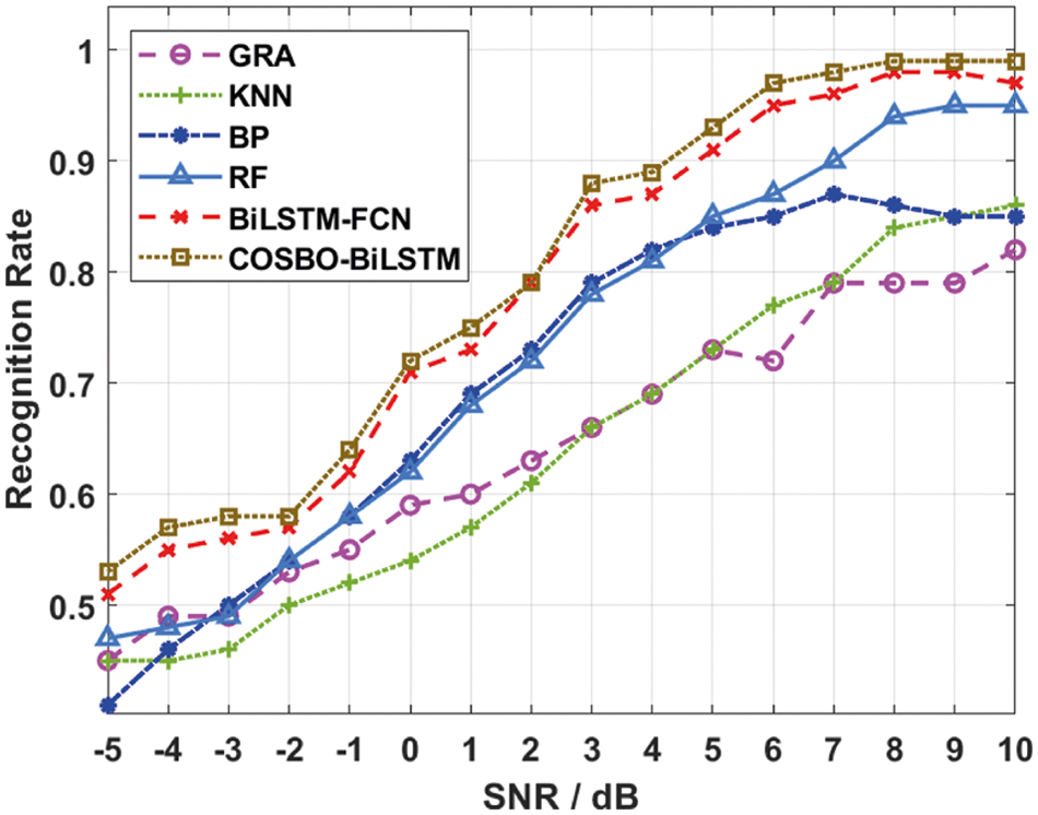
Figure 10: RR analysis of COSBO-BiLSTM model with existing techniques

5  Conclusion

In this study, a new COSBO-BiLSTM technique is derived to classify the different kinds of digitally modulated signals in communication systems. The proposed COSBO-BiLSTM technique comprises three stages of operations as SFD based feature extraction, BiLSTM-FCN based modulation signal classification, and COSBO based hyperparameter optimization. The utilization of COSBO algorithm helps to considerately improve the overall classification efficiency of the BiLSTM-FCN technique. For examining the better outcomes of the COSBO-BiLSTM technique, a detailed experimental analysis takes place and the results are inspected under several aspects. The experimental results highlighted that the COSBO-BiLSTM technique has accomplished improved performance over the existing techniques. In future, advanced feature extraction techniques can be employed to improve the modulation signal classification performance.

Acknowledgement: The authors would like to acknowledge the support of Prince Sultan University for paying the Article Processing Charges (APC) of this publication.

Funding Statement: The authors extend their appreciation to the Deanship of Scientific Research at King Khalid University for funding this work under Grant Number (RGP 1/279/42). https://www.kku.edu.sa.

Conflicts of Interest: The authors declare that they have no conflicts of interest to report regarding the present study.

References

 1.  H. Li and M. Li, “Analysis of the pattern recognition algorithm of broadband satellite modulation signal under deformable convolutional neural networks,” PLoS ONE, vol. 15, no. 7, pp. e0234068, 2020. [Google Scholar]

 2.  I. F. Akyildiz, J. M. Jornet and S. Nie, “A new CubeSat design with reconfigurable multi-band radios for dynamic spectrum satellite communication networks,” Ad Hoc Networks, vol. 86, pp. 166–178, 2019. [Google Scholar]

 3.  L. X. Yu, L. Min, W. J. Yuan, O. Jian and H. Q. Quan, “Average symbol error rate for integrated satellite-terrestrial cooperative transmission with interference,” Acta Physica Sinica, vol. 68, no. 12, pp. 128401, 2019. [Google Scholar]

 4.  C. T. Shi, “Signal pattern recognition based on fractal features and machine learning,” Applied Sciences, vol. 8, no. 8, pp. 1327, 2018. [Google Scholar]

 5.  K. Liu, X. Zhang and Y. Chen, “Extraction of coal and gangue geometric features with multifractal detrending fluctuation analysis,” Applied Sciences, vol. 8, no. 3, pp. 463, 2018. [Google Scholar]

 6.  L. Mingzhu, Z. Yue, S. Lin and D. Jingwei, “Research on recognition algorithm of digital modulation by higher order cumulants,” in 2014 Fourth Int. Conf. on Instrumentation and Measurement, Computer, Communication and Control, Harbin, China, pp. 686–690, 2014. [Google Scholar]

 7.  J. Zhang, X. Wang and X. Yang, “A method of constellation blind detection for spectrum efficiency enhancement,” in 2016 18th Int. Conf. on Advanced Communication Technology (ICACT), Pyeongchang Kwangwoon Do, South Korea, pp. 148–152, 2016. [Google Scholar]

 8.  M. D. Z. Hossain, F. Sohel, M. F. Shiratuddin and H. Laga, “A comprehensive survey of deep learning for image captioning,” ACM Computing Surveys, vol. 51, no. 6, pp. 1–36, 2019. [Google Scholar]

 9.  T. Tuncer, S. Dogan and A. Subasi, “Surface EMG signal classification using ternary pattern and discrete wavelet transform based feature extraction for hand movement recognition,” Biomedical Signal Processing and Control, vol. 58, pp. 101872, 2020. [Google Scholar]

10. Y. Xu, D. Li, Z. Wang, Q. Guo and W. Xiang, “A deep learning method based on convolutional neural network for automatic modulation classification of wireless signals,” Wireless Networks, vol. 25, no. 7, pp. 3735–3746, 2019. [Google Scholar]

11. X. Zha, H. Peng, X. Qin, G. Li and S. Yang, “A deep learning framework for signal detection and modulation classification,” Sensors, vol. 19, no. 18, pp. 4042, 2019. [Google Scholar]

12. F. Wang, S. Huang, H. Wang and C. Yang, “Automatic modulation classification exploiting hybrid machine learning network,” Mathematical Problems in Engineering, vol. 2018, pp. 1–14, 2018. [Google Scholar]

13. S. Peng, H. Jiang, H. Wang, H. Alwageed, Y. Zhou et al., “Modulation classification based on signal constellation diagrams and deep learning,” IEEE Transactions on Neural Networks and Learning Systems, vol. 30, no. 3, pp. 718–727, 2019. [Google Scholar]

14. Y. Wang, H. Zhang, Z. Sang, L. Xu, C. Cao et al., “Modulation classification of underwater communication with deep learning network,” Computational Intelligence and Neuroscience, vol. 2019, pp. 1–12, 2019. [Google Scholar]

15. A. Ali, F. Yangyu and S. Liu, “Automatic modulation classification of digital modulation signals with stacked autoencoders,” Digital Signal Processing, vol. 71, pp. 108–116, 2017. [Google Scholar]

16. A. Güner, Ö. F. Alçin and A. Şengür, “Automatic digital modulation classification using extreme learning machine with local binary pattern histogram features,” Measurement, vol. 145, pp. 214–225, 2019. [Google Scholar]

17. P. Wu, B. Sun, S. Su, J. Wei, J. Zhao et al., “Automatic modulation classification based on deep learning for software-defined radio,” Mathematical Problems in Engineering, vol. 2020, pp. 1–13, 2020. [Google Scholar]

18. S. Zhou, Z. Yin, Z. Wu, Y. Chen, N. Zhao et al., “A robust modulation classification method using convolutional neural networks,” EURASIP Journal on Advances in Signal Processing, vol. 2019, no. 1, pp. 21, 2019. [Google Scholar]

19. Y. Lin, Y. Tu, Z. Dou and Z. Wu, “The application of deep learning in communication signal modulation recognition,” in 2017 IEEE/CIC Int. Conf. on Communications in China (ICCC), Qingdao, pp. 1–5, 2017. [Google Scholar]

20. Y. S. Liang, “Fractal dimension of riemann-liouville fractional integral of 1-dimensional continuous functions,” Fractional Calculus and Applied Analysis, vol. 21, no. 6, pp. 1651–1658, 2018. [Google Scholar]

21. M. Khan, H. Wang, A. Riaz, A. Elfatyany and S. Karim, “Bidirectional LSTM-RNN-based hybrid deep learning frameworks for univariate time series classification,” The Journal of Supercomputing, vol. 77, no. 7, pp. 7021–7045, 2021. [Google Scholar]

22. S. H. S. Moosavi and V. K. Bardsiri, “Satin bowerbird optimizer: A new optimization algorithm to optimize ANFIS for software development effort estimation,” Engineering Applications of Artificial Intelligence, vol. 60, pp. 1–15, 2017. [Google Scholar]

23. T. Wangkhamhan, “Adaptive chaotic satin bowerbird optimisation algorithm for numerical function optimisation,” Journal of Experimental & Theoretical Artificial Intelligence, vol. 33, no. 5, pp. 719–746, 2021. [Google Scholar]

24. Q. Wu and M. Shafiee, “Modeling and optimization of SOFC based on metaheuristics,” International Journal of Electrochemical Science, vol. 15, pp. 11008–11023, 2020. [Google Scholar]

This work is licensed under a Creative Commons Attribution 4.0 International License, which permits unrestricted use, distribution, and reproduction in any medium, provided the original work is properly cited.