DOI:10.32604/cmc.2022.024563
| Computers, Materials & Continua DOI:10.32604/cmc.2022.024563 | |
| Article |
Solving Cauchy Issues of Highly Nonlinear Elliptic Equations Using a Meshless Method
Department of Mechanical Engineering, National United University, Miaoli, 360302, Taiwan
*Corresponding Author: Chih-Wen Chang. Email: cwchang@nuu.edu.tw
Received: 22 October 2021; Accepted: 15 December 2021
Abstract: In this paper, we address 3D inverse Cauchy issues of highly nonlinear elliptic equations in large cuboids by utilizing the new 3D homogenization functions of different orders to adapt all the specified boundary data. We also add the average classification as an approximate solution to the nonlinear operator part, without requiring to cope with nonlinear equations to resolve the weighting coefficients because these constructions are owned many conditions about the true solution. The unknown boundary conditions and the result can be retrieved straightway by coping with a small-scale linear system when the outcome is described by a new 3D homogenization function, which is right to find the numerical solutions with the errors smaller than the level of noise being put on the over-specified Neumann conditions on the bottom of the cuboid. Besides, note that the new homogenization functions method (HFM) does not require dealing with the regularization and highly nonlinear equations. The robustness and accuracy of the HFM are verified by comparing the recovered results of several numerical experiments to the exact solutions in the entire region, even though a very large level of noise 50% is imposed on the over specified Neumann conditions. The numerical errors of our scheme are in the order of O(10−1)–O(10−4).
Keywords: Inverse cauchy problems; homogenization functions method (HFM); 3D highly nonlinear elliptic equations; 3D homogenization functions
In several past decades, lots of researchers utilized mesh methods and meshless approaches to tackle inverse Cauchy issues of linear elliptic equations; however, a few researchers can cope with inverse Cauchy issues of nonlinear elliptic equations. As we all known, inverse Cauchy issues of nonlinear elliptic equations play very pivotal roles in several engineering and scientific domains. These equations occur in the vibration of a structure, the acoustic cavity issue, the radiation wave, the scattering of a wave, heat conduction in fins, semiconductor structures, electrostatic analysis, neutron diffusion problems, advection–diffusion problems, steady-state groundwater flow and so forth.
For inverse Cauchy issues of linear elliptic equations, Marin et al. [1] proposed the numerical implementation of the conjugate gradient method (CGM) was accomplished by employing the boundary element method (BEM), which needs the discretisation of the boundary merely. They also claimed that Cauchy issues for two-dimensional (2D) Helmholtz-type equation were inverse boundary value issues and therefore the BEM was a very suitable approach for solving such improperly posed issues. However, the numerical results with noisy data are not good. Later, Marin et al. [2] addressed an iterative method on the basis of the Landweber algorithm in combination with the BEM for dealing with the Cauchy issue for 2D Helmholtz-type equations; nevertheless, the drawbacks of the Landweber scheme consisted of the relatively large numbers of iterations required to resolve the issue in comparison with the other regularization approaches. After that, the method of fundamental solutions (MFS) was utilized to solve the Cauchy issue associated with 2D Helmholtz-type equations [3]. Their numerical results showed that the present approach was convergent with respect to increasing the number of source points. Wei et al. [4] combined the MFS with three regularization techniques to resolve Cauchy issues of elliptic differential operators. Note that the use of more Cauchy conditions greatly improved the accuracy of the approximate solution; however, their strategy was complex. Qin et al. [5] tackled the highly ill-posed Cauchy issue for the modified Helmholtz equation was firstly transformed into a moment problem by using the Green's formula. From the numerical verifications, note that their proposed method was stable and efficient. Then, Qin et al. [6] utilized the quasi-reversibility and the truncation methods to solve a Cauchy issue for the modified Helmholtz equation in a rectangular domain and obtained stable convergence estimates. However, they did not compare with other available techniques, such as the regularized BEM, MFS, CGM. After that, Fan et al. [7] adopted the generalized finite difference method (GFDM) for solving inverse Cauchy issues. In Cauchy issues, part of the boundary data was missing and the numerical simulation may become very unstable. Besides, different levels of noise were added into the boundary conditions to demonstrate the stability of the GFDM; nevertheless, they used small noises to test those examples. Of late, Liu [8] has addressed a homogenized function skill by including the initial condition/boundary conditions/supplementary condition to simplify the governing equations for the recovery of a space-time–dependent heat source. Then, he employed the Pascal polynomials or the eigenfunctions to expanded the trial solutions. Besides, he also mentioned that the eigenfunction method was slightly better than the polynomial method. Later, Liu [9] proposed a multiple/scale/direction Trefftz expansion method (MSDTM) to solve the 3D Helmholtz equation in an arbitrary domain with an irregular boundary, and the solutions obtained were quite accurate. Later, Liu [10] also utilized a homogenized function technique to solve the initial condition/boundary conditions and supplementary data for the recovery of time/space-dependent heat sources. Although the supplementary data were contaminated by a large noise 20%, their methods are quite simple, stable and accurate. Liu et al. [11] the original multi-quadric radial basis function (MQ-RBF) was modified by introducing the multiple-scale method in the expansion of trial solution, of which the multiple-scale is determined a priori by the collocation points and source points, such that the column norms of the coefficient matrix are equal. Note that the accuracy in the solution of the inverse Cauchy issue in a doubly-connected domain was not as good as that for the simply-connected inverse Cauchy issues. Wang et al. [12] applied a regularized indirect BEM formulation for the solution of 3D inverse heat conduction issues. They claimed that the present method is computationally efficient, robust, accurate, stable with the decreasing noisy level in the input data. Liu et al. [13] developed a quite simple MSDTM to solve the inverse Cauchy issues of 3D modified Helmholtz equation in an arbitrary bounded area, which offered quite accurate solution. Although for the highly ill-posed inverse Cauchy issues in the 3D irregular area, the MSDTM performed well to retrieve the unknown boundary conditions despite a high level of noise. Liu et al. [14] resolved an inverse geometry problem (IGP) of the Poisson equation in an arbitrary doubly-connected plane area to retrieve an unknown inner boundary. However, the proposed homogenization/boundary function algorithm was limited to tackle the IGP with analytic boundary value functions, which were given explicitly. Later, Liu et al. [15] solved the highly ill-posed inverse Cauchy problems of the steady-state diffusion-convection-reaction equation by using the energy RBF. They also mentioned the weighting factors played the regularization role as the right pre-conditioner to diminish the ill-posed behavior of the inverse Cauchy issue against large noises being imposed on the data.
For inverse Cauchy issues of nonlinear elliptic equations, Essaouini et al. [16] utilized a numerical iterative boundary element approach to solve a class of nonlinear elliptic inverse issue. The scheme was implemented with various relaxation parameters. After that, Liu et al. [17] employed a variable transformation and the mixed group-preserving scheme (MGPS) to retrieve the missing information on the top side very well for a nonlinear inverse Cauchy issue. Later, Yeih et al. [18] proposed the double iteration process to cope with the Cauchy inverse issue of a nonlinear heat conduction equation. Numerical results show that this scheme is efficient and can acquire accurate enough results for a nonlinear ill-posed inverse issue. Liu [19] solved the nonlinear inverse Cauchy issue defined in an arbitrary doubly connected domain with a simple direct integration algorithm without requiring of any iteration. Apart from that, Zhang et al. [20] used a filtering function method to solve a Cauchy problem for semi-linear elliptic equation. Finally, they computed the regularization solution by constructing an iterative algorithm and obtained some stable and feasible results; however, this approach was complicated. Then, Tran et al. [21] addressed a regularization scheme to a quasi-linear elliptic Cauchy issue. They stressed that the regularized problem is well-posed, and its solution converged to the exact solution strongly in L2 where some a priori assumptions were pondered. Nevertheless, they did not show how to choose the optimal regularization parameter. After that, Liu et al. [22] tackled the nonlinear inverse Cauchy issue of the nonlinear elliptic type equation in an arbitrary doubly-connected plane area to retrieve the unknown inner boundary data. Liu et al. [23] tackled the Cauchy issues of the 3D nonlinear elliptic equations in cuboids by employing the superposition of homogenization functions method (SHFM). Upon comparing with the MGPS, they revealed that the SHFM can tackle the Cauchy issue in a large size of the cuboid, and furthermore, the SHFM was more accurate than the MGPS. Later, Liu et al. [24] addressed a simple and effective numerical skill, which aims to accurately and quickly deal with the thin plate bending issues. On the basis of the given boundary data, they established the thin plate homogenization function and derived a family of two-parameter homogenization functions. Liu et al. [25] solved the 3D inverse Cauchy problems of the elliptic type linear PDEs in the closed walled shells to retrieve the unknown inner boundary conditions. Several examples of the Laplace equation, the Helmholtz equation, the modified Helmholtz equation, the Poisson equation, a strong convection diffusion equation and a varying coefficient elliptic equation, confirmed the efficiency and accuracy of the presented numerical scheme. Liu et al. [26] coped with two Stefan problems. The first problem retrieved an unknown moving boundary by specifying the Cauchy boundary conditions on a fixed left-end. The second problem revealed a time-dependent heat flux on the left-end, such that a desired moving boundary can be achieved. Numerical instances, including non-smooth ones, confirm that the new approaches were simple and robust against large noise. Lin et al. [27] resolved the parameters identification issue in a nonlinear heat equation with homogenization functions as the bases. The proposed methods did not require iteration and solving nonlinear equations because the unknown heat conductivities were recovered from the solutions of linear systems. About the recent developments in the field of numerical simulation and stability as well as its applications, Mahdy and his coworkers have used many new methods to deal with those problems, such as the time-fractional Fokker–Planck equation [28], the isoperimetric variational problems [29], the nonlinear biochemical reaction model and nonlinear Emden-Fowler system [30], the fractional-order biological systems [31], the dynamical behaviors of nonlinear Coronavirus (COVID-19) model [32], a nonlinear fractional tumor-immune model [33], the fractional order Klein-Gordon equation [34], the Rubella ailment disease model [35], and the fractional nonlinear rubella ailment disease model [36]. After that, Iqbal and his coworkers have utilized three approaches to tackle three issues, such as the second order coupled nonlinear Schrödinger equations [37], nonlinear waves propagation and stability analysis for planar waves [38], and time fractional Black–Scholes model [39].
The current study owns a novelty by establishing a new 3D homogenization functions to demolish the boundary conditions on a partial portion of the cuboid, which is not published in the literature. In addition, the new homogenization functions scheme does not require to tackle the highly nonlinear equations and regularization. This article is organized as follows. Section 2 illustrates a formation skill from the low-dimensional homogenization function to the high-dimensional homogenization function. Then, in Section 3 we display the shape functions into the 3D homogenization function so that we can produce a family of 3D homogenization functions as the foundations of the solution of the 3D highly nonlinear Cauchy issue. Four numerical experiments of the Cauchy issues of the 3D highly nonlinear elliptic equations are shown in Section 4. At last, some conclusions are drawn in Section 5.
2 A New Homogenization Function
One kind Cauchy issue of the non-homogeneous and nonlinear elliptic equation is addressed in a 3D cuboid
where F is a first-order nonlinear operator, and H is another first-order nonlinear operator.
Nevertheless, the Neumann data
To establish the 3D homogenization function, we employ a sequential formation skill by beginning from the 1D boundary value problem (BVP):
where F is a second-order nonlinear differential operator.
Let
where
Indicate
The BVP with homogeneous boundary data are shown as follows:
Then, we ponder the 2D BVP:
Letting
which supersedes the constants
Denote
and in accordance with the following compatibility conditions:
we can certify
Hence, we can generate the 2D homogenization function for the 2D BVP:
Because of
with the aid of the variable conversion from
As well, we can establish the 3D homogenization function by beginning from the 2D homogenization function. We present a new scheme of the 3D highly nonlinear Cauchy issues by utilizing the superposition of the 3D homogenization functions.
Note that the given functions
The first four boundary data are functions of
which gratifies the first four boundary data in Eq. (2):
in which the compatible conditions
We employ the normalized coordinates to obtain a generalization of Eq. (21):
and the pth order shape functions:
in which the minimal prerequisites of
we use the simplest ones:
Hence, the k th order partial homogenization function can be shown as follows:
Utilizing the characters in Eq. (25), we can verify that the above
We can produce the p th order 3D homogenization function to fit the last two Cauchy data
and we can justify
The first four properties can be verified employing other consistent data in Eq. (20) and the following consistent data when the last two properties forthright track from Eq. (28):
Hence, assuming that
we can acquire the simplest solution of the 3D highly nonlinear Cauchy issue in the cuboid, of which
Eq. (32) is accustomed to promise that
We can inquire Eq. (31) to gratify the governing Eq. (1) and assume at the q interior points of
where in the nonlinear portion, we can use the average
as its argument. c is the highest order of the homogenization functions and
Advantages of this proposed algorithm are no iteration, against large noise, for large domain and no need of regularization to deal with the 3D highly nonlinear Cauchy issue. In addition, the computational complications of the current approach are about
4 Numerical Experiments of Highly Nonlinear Cauchy Problems
Since the Neumann data
where r denotes the intensity of noise and
In addition, the often utilized absolute error and relative error, we ponder a root-mean-square-error defined by
to estimate the accuracy of numerically retrieved boundary datum
Let (xi, yj), i = 1,…,N1, j = 1,…,N2 be the points on the plane z = f, where we compare the exact solution
The numerically computed order of convergence (COC) is approximated by
All the computational schemes were implemented to the Fortran code on the Microsoft Developer Studio platform in OS Windows 10 (64 bit) with i3-4160 3.60 GHz CPU and 16 GB memory.
We ponder a highly nonlinear one with
where the exact solution is
and thus,
We utilize
We draw the maximum errors of the numerical results of
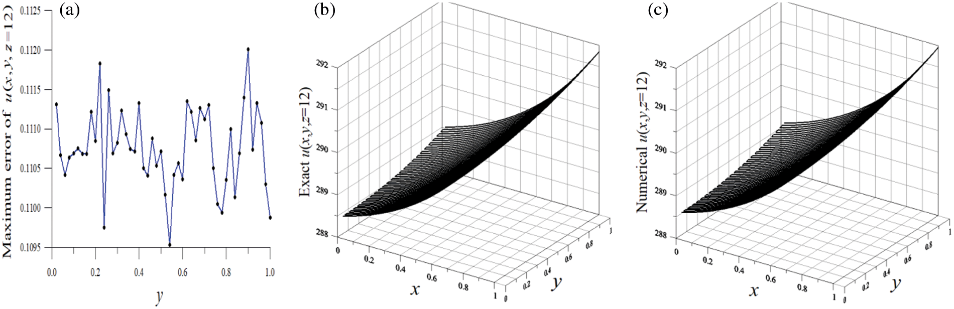
Figure 1: For example 1 of the 3D Cauchy issue of highly nonlinear equation, (a) displaying maximum errors with large noise effect, (b) exact solution and (c) numerical solution with large noise effect
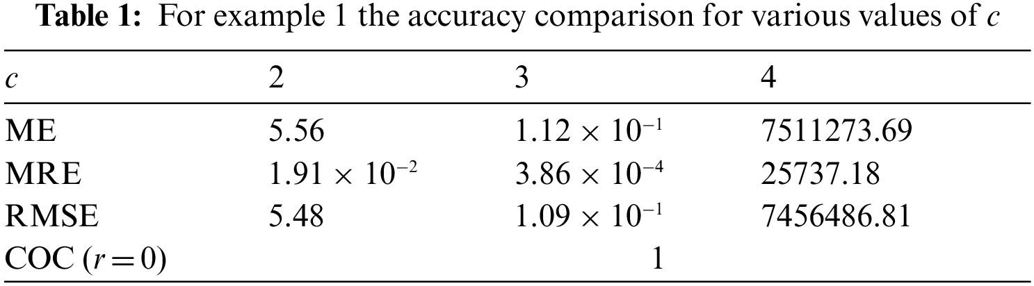
In Tab. 1, When we use
We deliberate another highly nonlinear one with
where the exact solution is assumed to be
and hence,
We sketch the maximum errors of the numerical results of
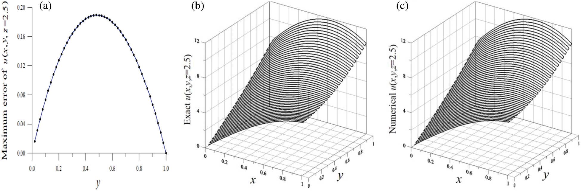
Figure 2: For example 2 of the 3D Cauchy issue of highly nonlinear equation, (a) displaying maximum errors with large noise effect, (b) exact solution and (c) numerical solution with large noise effect
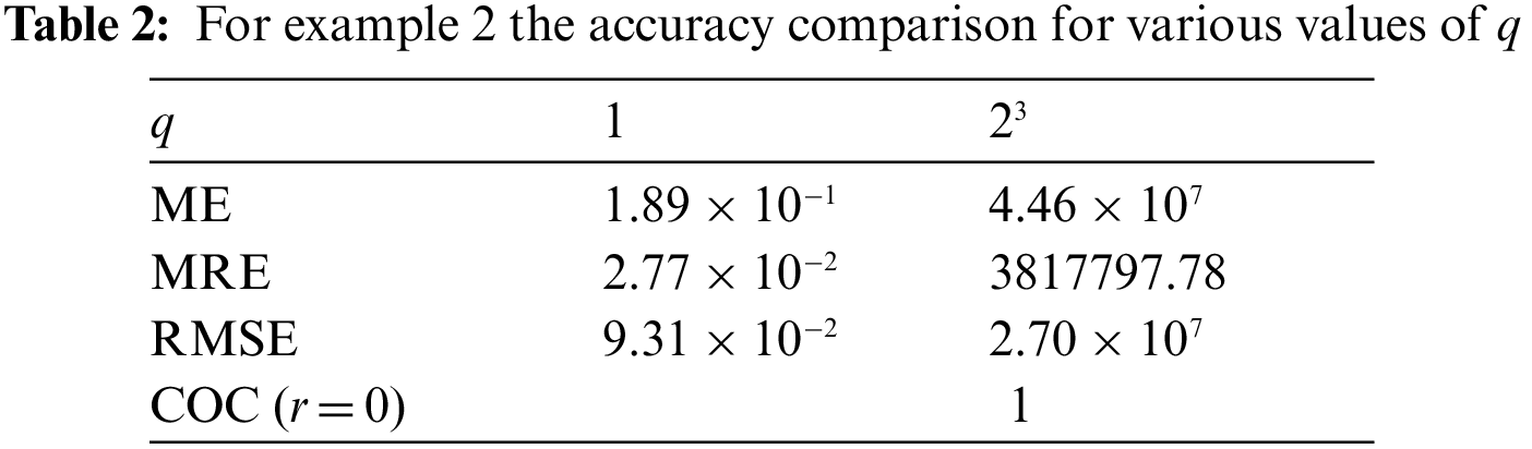
In Tab. 2, the ME, the MRE and the RMSE are listed for various values of q, when we take
We consider a highly nonlinear one with
where the exact solution is
and therefore,
Under the following parameters
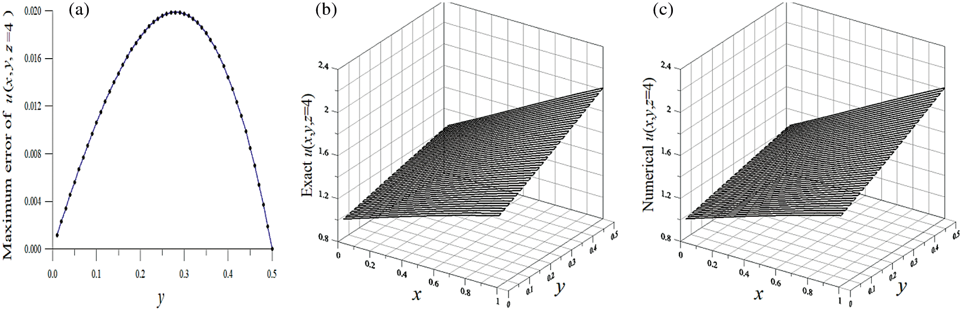
Figure 3: For example 3 of the 3D Cauchy issue of highly nonlinear equation, (a) displaying maximum errors with large noise effect, (b) exact solution and (c) numerical solution with large noise effect
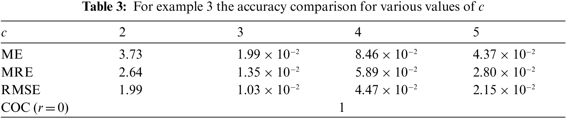
In Tab. 3, the ME, the MRE and the RMSE are listed for various values of c, when we take
Finally, we contemplate another highly nonlinear one with
where the exact solution is
and
Under the following parameters
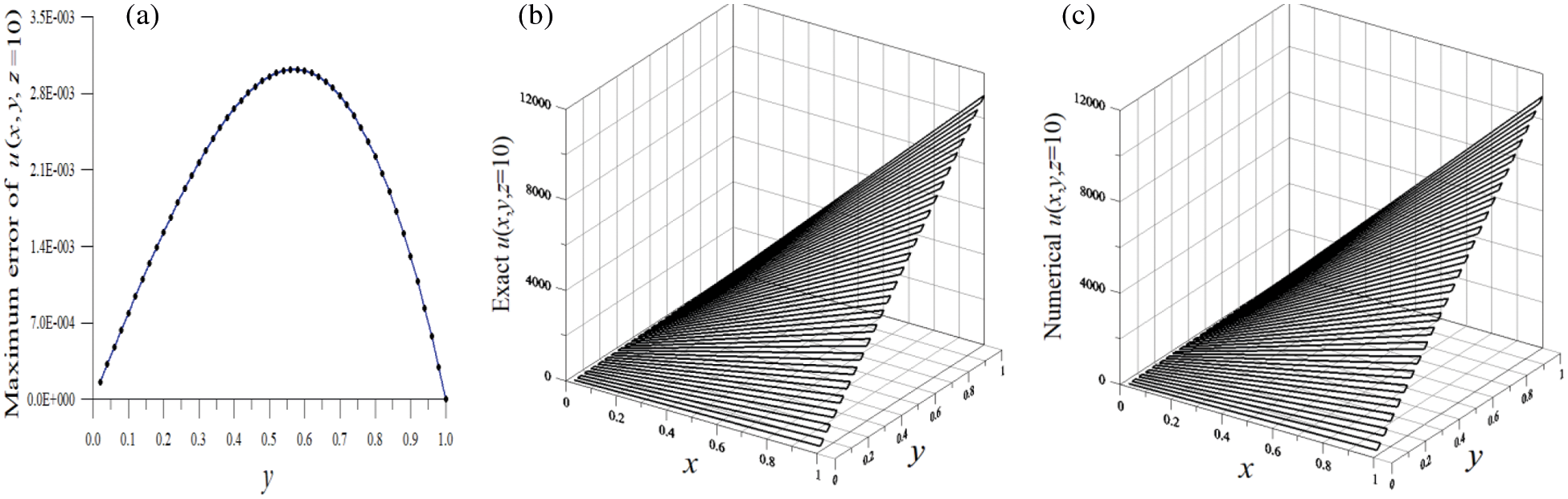
Figure 4: For example 4 of the 3D Cauchy issue of highly nonlinear equation, (a) displaying maximum errors with large noise effect, (b) exact solution and (c) numerical solution with large noise effect
We have addressed a new meshless approach to tackle the Cauchy issues of the 3D nonlinear elliptic equations in cuboids in this article. In the presently proposed homogenization functions method, we could construct the different-order 3D homogenization functions to fit all the specified boundary data, including the Neumann one in the whole area. We put in the average assortment as an approximate solution to the nonlinear operator section, without requiring to deal with nonlinear equations to decide the weighting coefficients since these establishments are owned many data about the true solution. The current scheme merely solving a small scale linear system is the simplest method to tackle the 3D highly nonlinear Cauchy issues, which is correct to reveal the numerical solutions with the errors smaller than the level of noise being placed on the over-specified Neumann data on the bottom of the cuboid. On the basis of those numerical experiments, we demonstrate that the proposed algorithm is applicable to the Cauchy issues of the 3D highly nonlinear elliptic equations in cuboids and very good computational efficient, and even for adding the large random noise up to 50%. The numerical errors of our method are in the order of O(10−1)–O(10−4). Furthermore, to the author's best knowledge, there has no report in the literature that the numerical methods for above-mentioned four issues can offer more accurate results than the present one. The present scheme can be extended to cope with the 3D fourth-order highly nonlinear steady state PDEs as shown in Fig. 5 and will be worked out in the future.

Figure 5: Frame work of 3D fourth-order highly nonlinear steady state PDEs by using the new HFM
Funding Statement: This work was financially supported by the National United University [Grant Numbers T110M20600].
Conflicts of Interest: The author declares that he has no conflicts of interest to report regarding the present study.
1. L. Marin and D. Lesnic, “The method of fundamental solutions for the Cauchy problem associated with two-dimensional Helmholtz-type equations,” Computers & Structures, vol. 83, no. 4–5, pp. 267–278, 2005. [Google Scholar]
2. L. Marin, L. Elliott, P. J. Heggs, D. B. Ingham, D. Lesnic et al., “Conjugate gradient-boundary element solution to the Cauchy problem for Helmholtz-type equations,” Computational Mechanics, vol. 31, no. 3–4, pp. 367–377, 2003. [Google Scholar]
3. L. Marin, L. Elliott, P. J. Heggs, D. B. Ingham, D. Lesnic et al., “BEM solution for the Cauchy problem associated with Helmholtz-type equations by the Landweber method,” Engineering Analysis with Boundary Elements, vol. 28, no. 9, pp. 1025–1034, 2004. [Google Scholar]
4. T. Wei, Y. C. Hon and L. Ling, “Method of fundamental solutions with regularization techniques for Cauchy problems of elliptic operators,” Engineering Analysis with Boundary Elements, vol. 31, no. 4, pp. 373–385, 2007. [Google Scholar]
5. H. H. Qin and D. W. Wen, “Tikhonov type regularization method for the Cauchy problem of the modified Helmholtz equation,” Applied Mathematics and Computation, vol. 203, no. 2, pp. 617–628, 2008. [Google Scholar]
6. H. H. Qin and T. Wei, “Quasi-reversibility and truncation methods to solve a Cauchy problem for the modified Helmholtz equation,” Mathematics and Computers in Simulation, vol. 80, no. 2, pp. 352–366, 2009. [Google Scholar]
7. C. M. Fan, P. W. Li and W. Yeih, “Generalized finite difference method for solving two-dimensional inverse Cauchy problems,” Inverse Problems in Science and Engineering, vol. 23, no. 5, pp. 737–759, 2015. [Google Scholar]
8. C. S. Liu, “To recover heat source g(x) + h(t) by using the homogenized function and solving rectangular differencing equations,” Numerical Heat Transfer, Part B Fundamentals, vol. 69, no. 4, pp. 351–363, 2016. [Google Scholar]
9. C. S. Liu, “A simple trefftz method for solving the Cauchy problems of three-dimensional Helmholtz equation,” Engineering Analysis with Boundary Elements, vol. 63, pp. 105–113, 2016. [Google Scholar]
10. C. S. Liu, “Homogenized functions to recover H(t)/H(x) by solving a small scale linear system of differencing equations,” International Journal of Heat and Mass Transfer, vol. 101, pp. 1103–1110, 2016. [Google Scholar]
11. C. S. Liu, W. Chen and Z. Fu, “A Multiple-scale MQ-RBF for solving the inverse Cauchy problems in arbitrary plane domain,” Engineering Analysis with Boundary Elements, vol. 68, pp. 11–16, 2016. [Google Scholar]
12. F. Wang, W. Chen, W. Qu and Y. Gu, “A BEM formulation in conjunction with parametric equation approach for three-dimensional Cauchy problems of steady heat conduction,” Engineering Analysis with Boundary Elements, vol. 63, pp. 1–14, 2016. [Google Scholar]
13. C. S. Liu, W. Qu, W. Chen and J. Lin, “A novel trefftz method of the inverse Cauchy problem for 3D modified Helmholtz equation,” Inverse Problems in Science and Engineering, vol. 25, no. 9, pp. 1278–1298, 2017. [Google Scholar]
14. C. S. Liu and D. Liu, “A homogenization boundary function method for determining inaccessible boundary of a rigid inclusion for the Poisson equation,” Engineering Analysis with Boundary Elements, vol. 86, pp. 56–63, 2018. [Google Scholar]
15. C. S. Liu and C. W. Chang, “An energy regularization of the MQ-RBF method for solving the Cauchy problems of diffusion-convection-reaction equations,” Communications in Nonlinear Science and Numerical Simulation, vol. 67, pp. 375–390, 2019. [Google Scholar]
16. M. Essaouini, A. Nachaoui and S. E. Hajji, “Numerical method for solving a class of nonlinear elliptic inverse problems,” Journal of Computational and Applied Mathematics, vol. 162, no. 1, pp. 165–181, 2004. [Google Scholar]
17. C. S. Liu and C. L. Kuo, “A Spring-damping regularization and a novel Lie-group integration method for nonlinear inverse Cauchy problems,” Computer Modeling in Engineering & Sciences, vol. 77, no. 1, pp. 57–80, 2011. [Google Scholar]
18. W. Yeih, I. Y. Chan, C. M. Fan, J. J. Chang and C. S. Liu. “Solving the Cauchy problem of the nonlinear steady-state heat equation using double iteration process,” Computer Modeling in Engineering & Sciences, vol. 99, no. 2, pp. 169–194, 2014. [Google Scholar]
19. C. S. Liu, “A Non-typical Lie-group integrator to solve nonlinear inverse Cauchy problem in an arbitrary doubly-connected domain,” Applied Mathematical Modelling, vol. 39, no. 13, pp. 3862–3875, 2015. [Google Scholar]
20. H. Zhang and X. Zhang, “Filtering function method for the Cauchy problem of a semi-linear elliptic equation,” Journal of Applied Mathematics and Physics, vol. 3, no. 12, pp. 1599–1609, 2015. [Google Scholar]
21. Q. V. Tran, M. Kirane, H. T. Nguyen and V. T. Nguyen, “Analysis and numerical simulation of the three-dimensional Cauchy problem for quasi-linear elliptic equations,” Journal of Mathematical Analysis and Applications, vol. 446, no. 1, pp. 470–492, 2017. [Google Scholar]
22. C. S. Liu and F. Wang, “A meshless method for solving the nonlinear inverse Cauchy problem of elliptic type equation in a doubly-connected domain,” Computers & Mathematics with Applications, vol. 76, no. 8, pp. 1837–1852, 2018. [Google Scholar]
23. C. S. Liu and C. W. Chang, “Solving the 3D Cauchy problems of nonlinear elliptic equations by the superposition of a family of 3D homogenization functions,” Engineering Analysis with Boundary Elements, vol. 105, pp. 122–128, 2019. [Google Scholar]
24. C. S. Liu, Q. Lin and J. Lin, “Simulating thin plate bending problems by a family of two-parameter homogenization functions,” Applied Mathematical Modelling, vol. 79, pp. 284–299, 2020. [Google Scholar]
25. C. S. Liu, Y. Zhang and F. Wang, “A homogenization function technique to solve the 3D inverse Cauchy problem of elliptic type equations in a closed walled shell,” Inverse Problems in Science and Engineering, vol. 29, no. 7, pp. 944–966, 2021. [Google Scholar]
26. C. S. Liu and J. R. Chang, “A homogenization method to solve inverse Cauchy–Stefan problems for recovering non-smooth moving boundary, heat flux and initial value,” Inverse Problems in Science and Engineering, vol. 29, no. 13, pp. 2772–2803, 2021. [Google Scholar]
27. J. Lin and C. S. Liu, “Recovering temperature-dependent heat conductivity in 2D and 3D domains with homogenization functions as the bases,” Engineering with Computers, 2021, DOI: https://doi.org/10.1007/s00366-021-01384-w. [Google Scholar]
28. A. M. S. Mahdy, “Numerical solutions for solving model time-fractional Fokker–Planck equation,” Numerical Methods for Partial Differential Equations, vol. 37, no. 2, pp. 1120–1135, 2021. [Google Scholar]
29. A. M. S. Mahdy and E. S. M. Youssef, “Numerical solution technique for solving isoperimetric variational problems,” International Journal of Modern Physics C, vol. 32, no. 1, pp. 2150002 (14 pages2021. [Google Scholar]
30. Y. A. Amer, A. M. S. Mahdy, T. T. Shwayaa and E. S. M. Youssef, “Laplace transform method for solving nonlinear biochemical reaction model and nonlinear Emden-Fowler system,” Journal of Engineering and Applied Sciences, vol. 13, no. 17, pp. 7388–7394, 2018. [Google Scholar]
31. Y. A. Amer, A. M. S. Mahdy and H. A. R. Namoos, “Reduced differential transform method for solving fractional-order biological systems,” Journal of Engineering and Applied Sciences, vol. 13, no. 20, pp. 8489–8493, 2018. [Google Scholar]
32. K. A. Gepreel, M. S. Mohamed, H. Alotaibi and A. M. S. Mahdy, “Dynamical behaviors of nonlinear coronavirus (COVID-19) model with numerical studies,” CMC: Computers Materials & Continua, vol. 67, no. 1, pp. 675–686, 2021. [Google Scholar]
33. A. M. S. Mahdy, M. Higazy and M. S. Mohamed, “Optimal and memristor-based control of a nonlinear fractional tumor-immune model,” CMC: Computers, Materials & Continua, vol. 67, no. 3, pp. 3463–3486, 2021. [Google Scholar]
34. M. M. Khader, N. H. Swetlam and A. M. S. Mahdy, “The chebyshev collection method for solving fractional order Klein-Gordon equation,” WSEAS Transactions on Mathematics, vol. 13, pp. 31–38, 2014. [Google Scholar]
35. A. M. S. Mahdy, K. A. Gepreel, K. Lotfy and A. A. El-Bary, “A numerical method for solving the rubella ailment disease model,” International Journal of Modern Physics C, vol. 32, no. 7, pp. 1–15, 2021. [Google Scholar]
36. A. M. S. Mahdy, M. S. Mohamed, K. Lotfy, M. Alhazmi, A. A. El-Bary et al., “Numerical solution and dynamical behaviors for solving fractional nonlinear rubella ailment disease model,” Results in Physics, vol. 24, pp. 1–10, 2021. [Google Scholar]
37. A. Iqbal, N. N. Abd Hamid, A. I. Md. Ismail and M. Abbas, “Galerkin approximation with quintic B-spline as basis and weight functions for solving second order coupled nonlinear Schrödinger equations,” Mathematics and Computers in Simulation, vol. 187, pp. 1–16, 2021. [Google Scholar]
38. A. Iqbal, M. J. Siddiqui, I. Muhi, M. Abbas and T. Akram, “Nonlinear waves propagation and stability analysis for planar waves at far field using quintic B-spline collocation method,” Alexandria Engineering Journal, vol. 59, no. 4 pp. 2695–2703, 2020. [Google Scholar]
39. T. Akram, M. Abbas, K. M. Abualnaja, A. Iqbal and A. Majeed, “An efficient numerical technique based on the extended cubic B-spline functions for solving time fractional Black–Scholes model,” Engineering with Computers, 2021, DOI: https://doi.org/10.1007/s00366-021-01436-1. [Google Scholar]
 | This work is licensed under a Creative Commons Attribution 4.0 International License, which permits unrestricted use, distribution, and reproduction in any medium, provided the original work is properly cited. |