Computers, Materials & Continua DOI:10.32604/cmc.2022.024604
Article

Bio-Inspired Computational Methods for the Polio Virus Epidemic Model

Fatimah Abdulrahman Alrawajeh1, F. M. Allehiany2, Ali Raza3,*, Shaimaa A. M. Abdelmohsen4, Tahir Nawaz Cheema5, Muhammad Rafiq6 and Muhammad Mohsin7

1Department of Mathematics, Faculty of Science College, Imam Abdulrahman Bin Faisal University (IAU), Dammam, 31441, Saudi Arabia
2Department of Mathematical Sciences, College of Applied Sciences, Umm Al-Qura University, P.O. Box 715, Makkah, 21955, Saudi Arabia
3Department of Mathematics, Govt. Maulana Zafar Ali Khan Graduate College Wazirabad, 52000, Punjab Higher Education Department (PHED) Lahore, 54000, Pakistan
4Department of Physics, College of Science, Princess Nourah bint Abdulrahman University, Riyadh 11671, Saudi Arabia
5Department of Mathematics, University of Gujrat, Gujrat, 50700, Pakistan
6Department of Mathematics, Faculty of Sciences, University of Central Punjab, Lahore, 54600, Pakistan
7Department of Mathematics, Technische Universitat Chemnitz, 6209111, Germany
*Corresponding Author: Ali Raza. Email: alimustasamcheema@gmail.com
Received: 24 October 2021; Accepted: 24 January 2022

Abstract: In 2021, most of the developing countries are fighting polio, and parents are concerned with the disabling of their children. Poliovirus transmits from person to person, which can infect the spinal cord, and paralyzes the parts of the body within a matter of hours. According to the World Health Organization (WHO), 18 million currently healthy people could have been paralyzed by the virus during 1988–2020. Almost all countries but Pakistan, Afghanistan, and a few more have been declared polio-free. The mathematical modeling of poliovirus is studied in the population by categorizing it as susceptible individuals (S), exposed individuals (E), infected individuals (I), and recovered individuals (R). In this study, we study the fundamental properties such as positivity and boundedness of the model. We also rigorously study the model’s stability and equilibria with or without poliovirus. For numerical study, we design the Euler, Runge–Kutta, and nonstandard finite difference method. However, the standard techniques are time-dependent and fail to present the results for an extended period. The nonstandard finite difference method works well to study disease dynamics for a long time without any constraints. Finally, the results of different methods are compared to prove their effectiveness.

Keywords: Poliovirus; modeling; stability results; computational methods

1  Introduction

Poliomyelitis, often termed polio, is a highly infectious viral disease and is also highly contagious. It is caused by poliovirus, a member of the genus Enterovirus of the family Picornaviridae. These viruses are small and have single-stranded ribonucleic acid (RNA) as their genetic material. They are classified into three kinds: serotypes 1, 2, and 3. Type 1 is the most frequent and the most lethal of viruses. Type 2 has not been found anywhere in the world since 1991. Polio is an exclusively human disease that is transmitted from person to person. Vaccination for polio is widely available now, and it is easy to culture when compared to other viruses. Various kinds of excruciating paralysis manifest differently, ranging from one of the most frequent to its most serious conditions. Historians have set down evidence of poliomyelitis in ancient times. The clinical features range from mild cases of respiratory illness, gastroenteritis, and malaise to severe forms of paralysis. This disease has been associated with debilitating abnormalities that have affected countless lives across the globe. Great scientists’ persistence and dedication help describe the viral structure in the 1900s. The World Health Organization (WHO) declared the Region of the Americas polio-free in 1994. Western Pacific was certified polio-free in 2000, followed by Europe in June 2002. In 2013, only Nigeria, Pakistan, and Afghanistan remained polio-endemic. Even after the worldwide elimination of polio, an outbreak is still very much possible. With the help of the WHO, all the governments worldwide are working to eradicate poliomyelitis. A highly infectious viral infection may cause paralysis, respiratory issues, or even death. Most polio infections are asymptomatic. On March 27, 2014, the WHO declared South-East Asia polio-free, ensuring that wild poliovirus spread stopped in 11 countries from Indonesia to India. This means that 80 % of the world's population lives in polio-free zones. More than 18 million formerly crippled individuals can now walk. Poor implementation strategies result in the spread of the virus. Wild poliovirus is the major reason for the endemic spread in Afghanistan and Pakistan. The inability to eradicate polio in these two countries may result in up to 200,000 additional cases each year in the next decade. That is why it is hard to say polio is gone for good. The polio eradication methods work only when they are implemented properly, which was proved by India's polio-free January 2011. In March 2014, the WHO declared India, the most difficult location in South-East Asia, polio-free. Polio is more likely among pregnant women, and it affects non-vaccinated youngsters severely. It is transmitted from one person to another orally. There is no cure for polio, but it can be prevented through vaccination. As 90 % of infected people have no symptoms, they go undiagnosed and become virus carriers. Since 1988, polio cases have decreased by 95 % globally. But two endemic nations, Pakistan and Afghanistan, are fighting to join the global immunization effort. In Pakistan, the COVID-19 curve shows a 2% positive rate for much of July–October, however, diseases like polio get more attention. On November 16, 2020, Pakistan had 81 polio cases, compared to 147 in 2019. Eliminating polio from Afghanistan, Pakistan, and Nigeria remains a major problem. The Pakistan national polio program organizes household-level vaccination programs. Poliomyelitis is a severe infectious illness. A gut virus attacks the brain and spinal cord nerve cells. A high-temperature headache characterizes fibromyalgia so that it may paralyze limbs or respiratory muscles. However, respiratory paralysis is uncommon. Polio can spread via food or water. It may also spread while altering an infected child's nappies. The virus enters through the nose or mouth, multiplies in the throat and intestinal tract, and then is absorbed and spread through the blood and lymph system. Anti-polio antibodies prevent the spread of the virus and provide lifetime protection. In 2009, only 48% and 57%, respectively, of children under five in Bangkalan and Bondowoso had antibodies against all three polioviruses. According to the Center for Disease Control (CDC), both districts had less than 80% vaccination coverage for regular immunization and more than 90 % for National Immunization Week. Thus, the number of nations with endemic diseases has declined from 125 in 2000 to three in 2012. World Polio Day is observed on October 24 every year. The WHO recognized the Americas, Europe, South Asia, and the Western Pacific as polio-free. Afghanistan, Pakistan, and Nigeria are the only countries where polio is still prevalent. Afghanistan and Pakistan are the only two nations where polio is an endemic problem. According to 2016 data, the virus is still circulating mostly in Afghanistan and Pakistan, sporadically transmitted to neighboring countries. In 2021, Ahmad et al. [1] worked on challenges and efforts related to polio during COVID-19 in Pakistan. Ataullahjan et al. [2] expressed a systematic review of polio eradication policies in Pakistan. Haqqi et al. [3] explored the impact of COVID-19 on the global polio eradication initiative in Pakistan. Nwogu et al. [4] overviewed the outbreak of polio in Kenya from 2013 to 2015. Bandyopadhyaya et al. [5] found the end game of polio eradication in final frontiers. Konopka-Anstadt et al. [6] evaluated a new oral vaccine for the eradication end game using codon deoptimization. Benissan et al. [7] introduced the poliovirus vaccine and the trivalent oral polio vaccine/bivalent oral polio vaccine in the African region. Lopalco [8] reviewed vaccine poliovirus circulation and its implications. Kabir et al. [9] generalized infection transmission of poliovirus epidemiology and possible risk factors in Pakistan. Akil et al. [10] interpreted the outbreaks and reemergence of poliovirus in war and affected areas. Patel et al. [11] presented the global introduction of inactivated polio vaccine. Nakamura et al. [12] explored the introduction period for inactivated polio vaccine environmental surveillance in sewage water. Bandyopadhyay et al. [13] explained polio’s present, past, and future regarding vaccination. Martinez-Bakker et al. [14] analyzed the historical facts and current challenges of poliomyelitis eradication. Singh et al. [15] reviewed polio literature and gave suitable measures to overcome it. Agarwal et al. [16] showed the modeling spread of polio with the role of vaccination. Jesus [17] described the modern history from epidemics to the eradication of poliomyelitis. The deterministic models are investigated using delay techniques as discussed in [18,19]. Hussain et al. [20] investigated the dynamics of pine wilt disease using the concept of sensitivity analysis. Raza et al. [21] studied the structure-preserving analysis of the epidemic model with necessary properties. More techniques related to epidemic models are given in [22,23]. The well-known results with different techniques are studied in [24–32]. The rest of the manuscript is organized as follows. Section 2 describes the modeling of polio. Section 3 discusses the numerical methods. Section 4 discusses the outcomes and future issues.

2  Modelling of Polio

For any time t, S: represents the class that is influenced by infection, E: represents the class that is disclosed by disease, I: represent an infective class, V: represents immunization class, A: represents the constant immigration rate of the human population, β: is the per unit time probability of infection transmission by infective population, Rβ: (0 < r ≤ 1): is the per unit time probability of infection transmission by exposed population, r: is the reduction in the exposed class due to transmission of infection, v: represents the proportion of recruits in the susceptible class moving to the vaccinated class, v1: is the number of exposed populations that are vaccinated, b: number of exposed people move to the infection class, µ: natural death of human population and α: disease death rate of the human population. Thus, a continuous model for people regarding polio is described in Fig. 1.

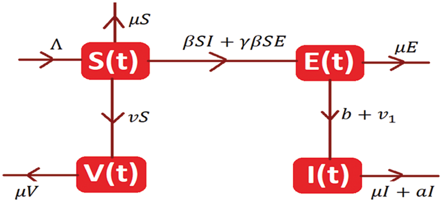
Figure 1: Spread map of polio

The system of differential equations is as follows:

S′(t)=A−βSI−rβSE−(µ+v)S,(1)

E′(t)=βSI+rβSE−(b+µ+v1)E,(2)

I′(t)=(b+v1)E−(µ+α)I,(3)

V′(t)=vS−µV.(4)

With initial condition S (0) ≥ 0; E (0) ≥ 0; I (0) ≥0; V (0) ≥ 0.

2.1 Model Properties

Theorem 1: Solutions (1–4) with initial conditions are positive for all t≥0.

Proof: By letting the Eq. (1),

S′=A−βSI−rβSE−(µ+v)S,S′≥−[βI+rβE+(µ+v)]S.

S(t)≥e∫−[βI+rβE+(µ+v)]dt≥0(5)

From Eq. (2),

E(t)≥e∫−E[rβS+(b+µ+v1)]≥0(6)

From Eq. (3)

I(t)≥e−(µ+α)t≥0(7)

From Eq. (4)

V(t)≥e−µt≥0(8)

Hence, the positivity of the desired system is proved.

Theorem 2: The solutions (S,E,I,V)ϵR+4 of the system (1–4) are bounded at any time t ≥ 0 and limit→∞SupN(t)≤Aμ.

Proof: let us consider the function as follows:

N(t)=S(t)+E(t)+I(t)+V(t).

dNdt+μN≤A.

The auxiliary equation is

limt→∞SupN(t)≤Aμ, as required.

2.2 Model Equilibria

The system admits two types of equilibria is as follows:

The disease-free equilibrium of the model is K 0=(Aμ+v,0,0,vμS).

The endemic equilibrium of the model is denoted by K1= (S*, E*, I*, V*).

S∗=(b+μ+v1)(μ+α)β(b+v1)+rβ(μ+α), E∗=A−(μ+v)S∗rβS∗+βS∗(b+v1μ+α), I∗=b+v1μ+αE∗, and V∗=vμS∗.

2.3 Reproduction Number

This section finds the reproduction number R0 by using the following generation matrix method. We introduce two types of matrices: the transition matrix and the second is transmission matrix.

[E′I′V′]=[rSββS0000000][EIV]−[b+μ+v100−b−v1μ+α000μ][EIV].

Here,

FG−1=[rβA(μ+v)(b+μ+v1)+βA(b+v1)(μ+v)(μ+α)(b+μ+v1)βA(μ+v)(μ+α)0000000].

The spectral radius of the FG−1 is called the reproduction number is as follows:

R0=βA(b+v1)(μ+v)(μ+α)(b+μ+v1)+rβA(μ+v)(b+μ+v1),

Where R1=βA(b+v1)(μ+v)(μ+α)(b+μ+v1) ,R2=rβA(μ+v)(b+μ+v1).

2.4 Local Stability

Theorem 3: The disease-free equilibrium K 0=(Aμ+v,0,0,vμS) is locally asymptotically stable if R0<1 otherwise unstable if R0>1.

Proof: Considering the function from the system (1–4) as follows:

The elements of the given Jacobean matrix at KO is as follows:

J(KO)=[−(μ+v)−rβAμ+V−βAμ+V00rβAμ+V−(b+μ+v1)βAμ+V00b+v1−(μ+α)0V00−μ].

J(KO−λI)=|−(μ+v)−λ−rβAμ+V−βAμ+V00rβAμ+V−(b+μ+v1)−λβAμ+V00b+v1−(μ+α)−λ0V00−μ−λ|=0.

We obtain the following results by applying Routh Hurwitz criteria for 2nd order.

A1>0,A2>0, if R0,R2<1, where A1=[(μ+α)+(b+μ+v1)(1−R2)], A2=(μ+α)(b+μ+v1)(1−R0).

Theorem 4: The endemic equilibrium K1= (S*, E*, I*, V*) is locally asymptotically stable if Ro>1.

Proof: The Jacobean matrix at K1=(S∗,E∗,I∗,V∗) is as follows:

J(K1)=[−βI∗−rβE∗−(μ+v)−rβS∗−βS∗0βI∗+rβE∗rβS∗−(b+μ+v1)βS∗00b+v1−(μ+α)0V00−μ].

|J(K1−λI)|=|−βI∗−rβE∗−(μ+v)−λ−rβS∗−βS∗0βI∗+rβE∗rβS∗−(b+μ+v1)−λβS∗00b+v1−(μ+α)−λ0V00−μ−λ|=0.

λ1=−μ<0,

−βI∗−rβE∗−(μ+v)−λ|rβS∗−(b+μ+v1)−λβS∗b+v1−(μ+α)−λ|−(βI∗+rβE∗)|−rβS∗−βS∗b+v1−(μ+α)−λ|=0.

Where A=βI∗+rβE∗+(μ+v)−rβS∗+(b+μ+v1)+(μ+α), B=−rβ2S∗I∗+βI∗(b+μ+v1)+βI∗(μ+α)+rβE∗(b+μ+v1)+rβE∗(μ+α)−rβS∗(μ+v)+(μ+v)(b+μ+v1)+(μ+α)(μ+v)−rβS∗(μ+α)+(b+μ+v1)(μ+α)−(βS∗)(b+v1)+rβ2S∗I∗, C=−rβ2S∗I∗(μ+α)+βI∗(b+μ+v1)(μ+α)−r2β2E∗S∗(μ+α)+rβE∗(b+μ+v1)(μ+α)−rβE∗S∗(b+v1)−rβS∗(μ+α)(μ+v)+(b+μ+v1)(μ+α)(μ+v)−(μ+v)βS∗(b+v1)+rβ2S∗I∗(μ+α)+r2β2E∗S∗(μ+α)+rβ2S∗E∗(b+v1).

Applying Routh-Hurwitz Criterion for 3rd order, A>0,D>0, and AC>D, if R0>1.

Hence the given system is locally asymptotically stable.

3  Numerical Methods

3.1 Euler Method

The Euler method for the Eqs. (1–4) is as follows:

Sn+1=Sn+h[A−βSnIn−rβSnEn−(μ+v1)Sn](9)

En+1=En+h[βSnIn+rβSnEn−(b+μ+v1)En](10)

In+1=In+h[(b+v1)En−(μ+α)In](11)

Vn+1=Vn+h[v1Sn−μVn](12)

Where “h” is represented by time step size.

3.2 Runge Kutta Method

The Runge Kutta method for the Eqs. (1–4) is as follows:

Stage 1

N1= h[v1Sn−μVn]

Stage 2

Stage 3

Stage 4

Final stage

Sn+1=Sn+16[K1+2K2+2K3+K4]En+1=En+16[L1+2L2+2L3+L4]In+1=In+16[M1+2M2+2M3+M4]Vn+1=Vn+16[N1+2N2+2N3+N4]}(13)

where “h” is represented by the time step size.

3.3 Nonstandard Finite Difference Method

The nonstandard finite difference (NSFD) could be developed for the system (1–4), the Eq. (1) of the polio epidemic model may be calculated as:

dSdt=A−βSI−rβSE−(μ+v1)S.

The decomposition of proposed method is as follows:

Sn+1=Sn+h[A−βSn+1In−rβSn+1En−(μ+v1)Sn+1].

Sn+1=Sn+hA1+hβIn+hrβEn+h(μ+v1)(14)

In the same way, we decompose the remaining system into proposed nonstandard finite difference (NSFD) method, like Eq. (14), as follows:

En+1=En+hβSnIn+hrβSnEn1+h(b+μ+v1)(15)

In+1=In+h((b+v1)En1+h(μ+α)(16)

Vn+1=Vn+hv1sn1+hμ(17)

where “h” is represented by time step size.

3.4 Linearization Process of Nonstandard Finite Difference (NSFD) Method

In this section, we shall present the theorem at the equilibria of the model for the process of linearization of the nonstandard finite difference (NSFD) method is as follows:

Theorem 5: The nonstandard finite difference (NSFD) method is stable if the eigenvalues of Eqs. (14–17) lie in the same unit circle, for any n≥0.

Proof: Consider the right-hand sides of the equation in (14–17) as functions L1, L2, L3, L4, as follows:

The elements of the Jacobian matrix are given as

J(S,E,I,V)=[∂L1∂S∂L1∂E∂L1∂I∂L1∂V∂L2∂S∂L2∂E∂L2∂I∂L2∂V∂L3∂S∂L3∂E∂L3∂I∂L3∂V∂L4∂S∂L4∂E∂L4∂I∂L4∂V].

The given Jacobian matrix at K 0=(Aμ+v,0,0,vμS) is as follows:

J(k0)=|11+h(μ+v1)−λ−(Aμ+v+hA)rhβ[1+h(μ+v1)]2−hβ(Aμ+v+hβ)[1+h(μ+v1)]20011−rhβ(Aμ+v)+h(b+μ+v1)−λhβ(Aμ+v)(1+rhβ(Aμ+v)+h(b+μ+v1))[1−rhβ(Aμ+v)+h(b+μ+v1)]200h(b+v1)1+h(μ+α)−λ0hv11+hμ0011+hμ−λ|=0.

λ1=11+hμ<1,

(μ+v(μ+v)−rhβA+(μ+v)h(b+μ+v1)−λ)(−λ)−(hβA((μ+v)+rhβA+(μ+v)h(b+μ+v1))[ (μ+v)−rhβA+(μ+v)h(b+μ+v1) ]2)(h(b+v1)1+h(μ+α)) = 0

λ2−μ+v(μ+v)−rhβA+(μ+v)h(b+μ+v1)(λ)−(hβA((μ+v)+rhβA+(μ+v)h(b+μ+v1))[ (μ+v)−rhβA+(μ+v)h(b+μ+v1) ]2)(h(b+v1)1+h(μ+α))=0.

Hence, by using the Mathematica software all the eigen values of the above Jacobian matrix lie in the unit circle if R0<1.Thus, the system (14–17) is stable.

Now, for endemic equilibrium (EE) K1= (S*, E*, I*, V*). The given Jacobian matrix is

λ1=11+hμ<1,

By using Mathematica software, the largest eigen value of the Jacobian is less than one, ultimately remaining will also lie in the unit circle when R0>1. Thus, endemic equilibrium is stable.

3.5 Numerical Results

For the analysis of the Eqs. (1) to (4), we use the values of the parameters which is presented in Tab. 1 is as follows:

3.6 Comparison Section

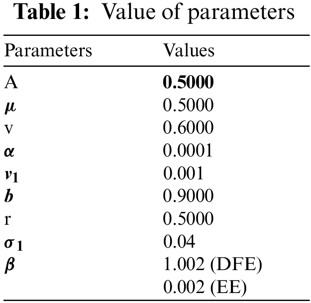
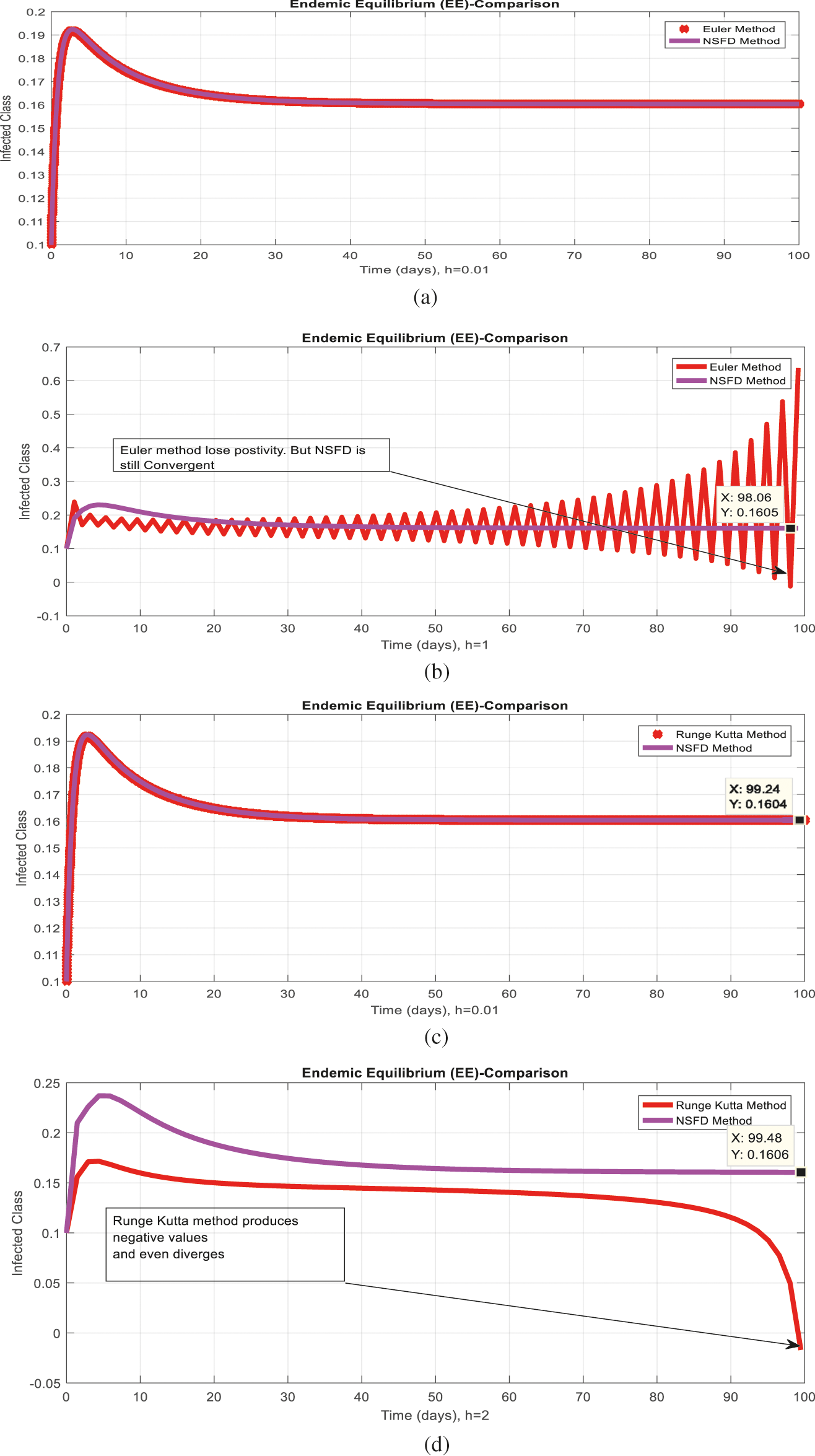
Figure 6: Comparison behavior (a) Infected class for endemic equilibrium (EE) with Euler and nonstandard finite difference (NSFD) methods at h=0.01 (b) Infected class for endemic equilibrium (EE) with Euler and nonstandard finite difference (NSFD) methods at h=1 (c) Infected class for endemic equilibrium (EE) with Runge Kutta and nonstandard finite difference (NSFD) methods at h=0.01 (d) Infected class for endemic equilibrium (EE) Runge Kutta and nonstandard finite difference (NSFD) methods at h=2

4  Results and Concluding Remarks

Figs. 2a and 2b show the simulation of the continuous model for both equilibria at any time t, using the ODE (45). Figs. 3a and 3b analyze the dynamics using the Euler method, which is consistent with the model's continuous behavior for the small-time step size. Unfortunately, the increasing time step size indicates the negativity and unboundedness of the results. However, this kind of analysis has no real relevance. In Figs. 4a and 4b, the Runge–Kutta method produces the same scenario as Euler, but comparatively much better. Figs. 5a and 5b show the actual behavior of the disease and is also valid for the long-term analysis. Figs. 6a and 6d show the effectiveness of the proposed method, such as nonstandard finite-difference. It also proves the positivity, boundedness, and dynamical consistency of the results. The study analyzes poliovirus modeling using analytical approaches and numerical techniques. The nonstandard finite difference (NSFD) scheme is a comfortable tool to analyze dynamical properties such as stability, positivity, and boundedness and shows the exact behavior of the continuous model. We shall extend this kind of analysis for all kinds of complex and nonlinear problems in the future.

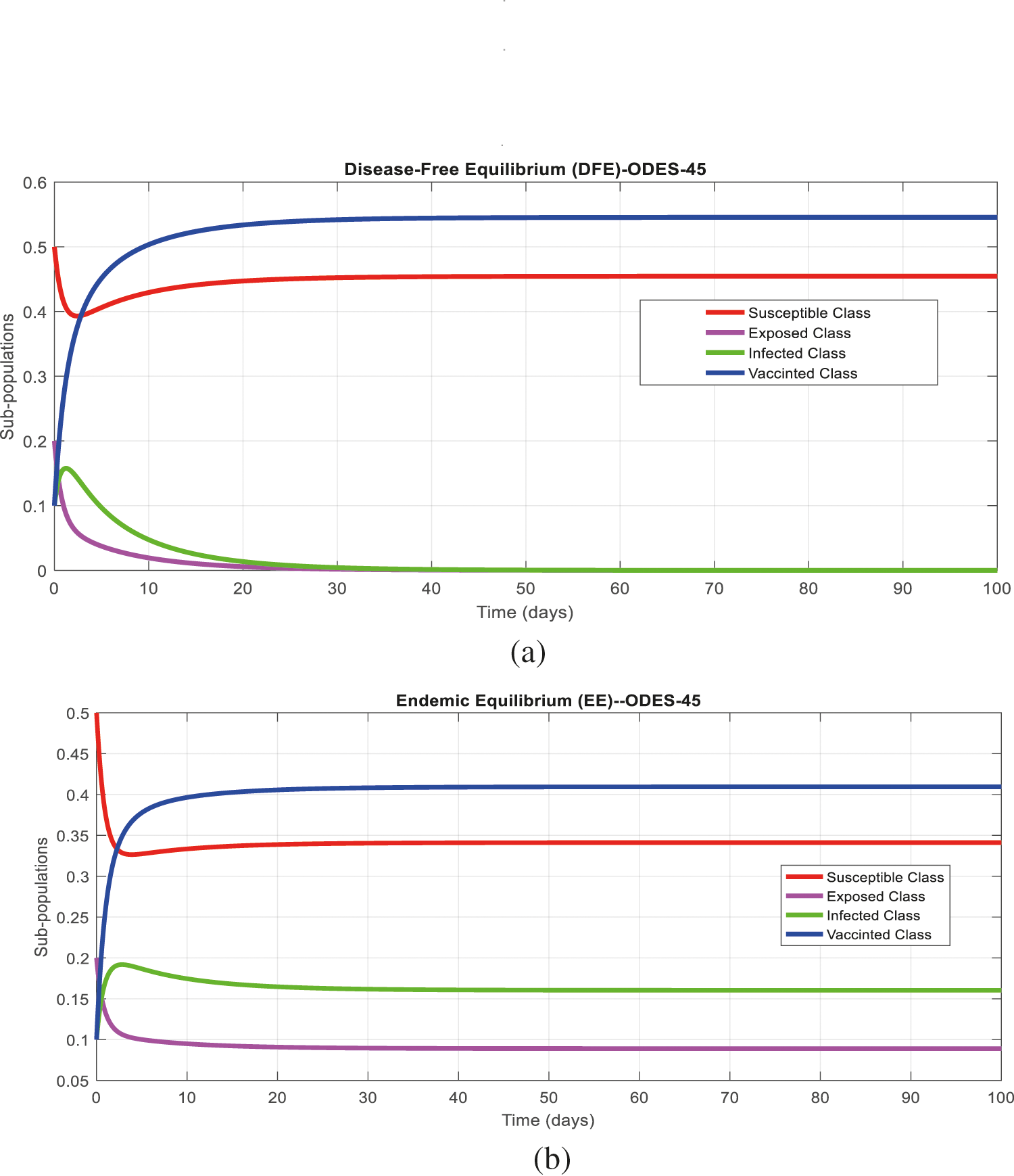
Figure 2: (a) Time plot for disease-free equilibrium (DFE) at any time t (b) Time plot for endemic equilibrium (EE) at any time t

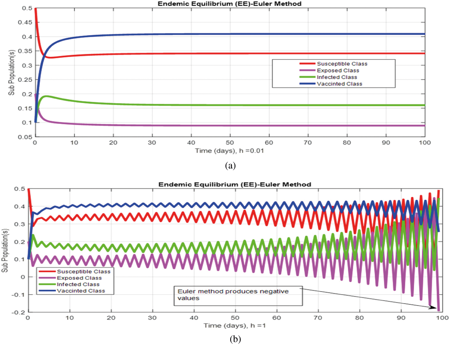
Figure 3: (a) (Convergent behavior) Sub-populations for endemic equilibrium (EE) at h=0.01. (b) (Divergent behavior) Sub-populations for endemic equilibrium (EE) at h=1

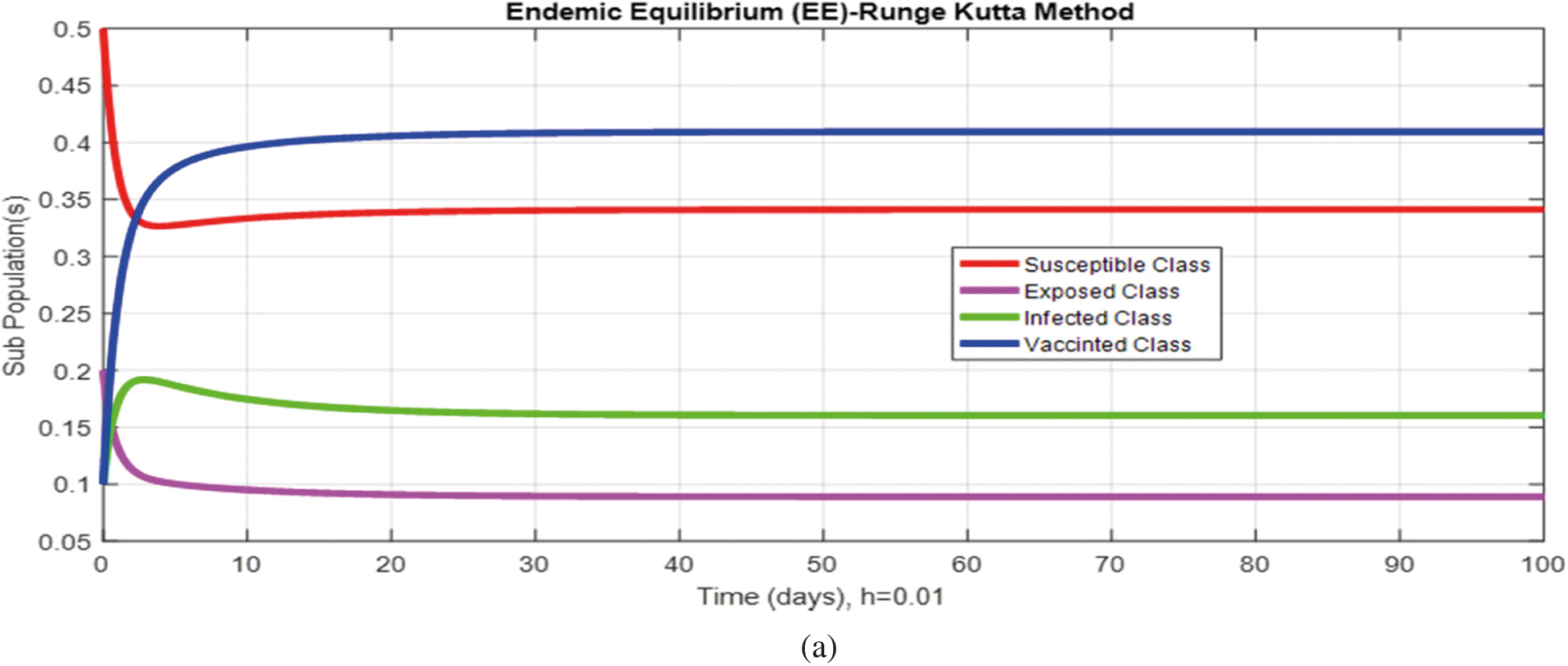
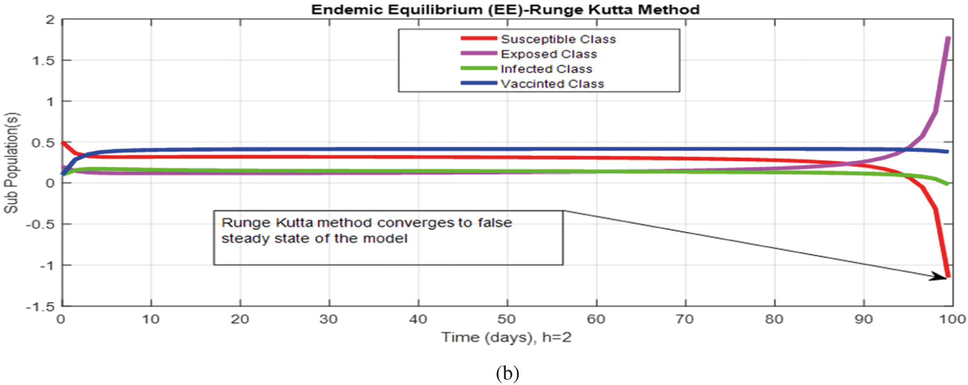
Figure 4: (a) (Convergent behavior) Sub-populations for endemic equilibrium (EE) at h=0.01 (b) (Divergent behavior) Sub-populations for endemic equilibrium (EE) at h=2

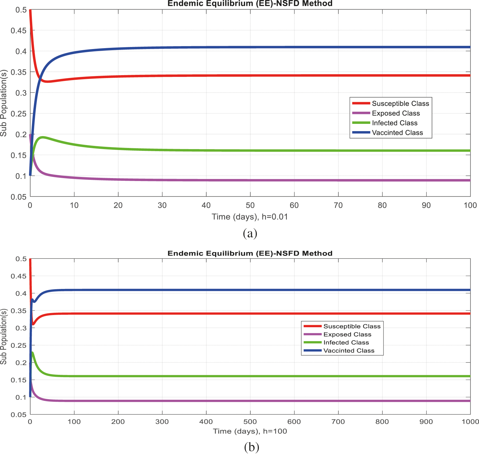
Figure 5: (a) (Convergent behavior) Sub-populations for endemic equilibrium (EE) at h=0.01 (b) Sub-populations for endemic equilibrium (EE) at h=100

Acknowledgement: The authors express their gratitude to Princess Nourah bint Abdulrahman University Researchers Supporting Project (Grant No. PNURSP2022R61), Princess Nourah bint Abdulrahman University, Riyadh, Saudi Arabia.

Funding Statement: The authors express their gratitude to Princess Nourah bint Abdulrahman University Researchers Supporting Project (Grant No. PNURSP2022R61), Princess Nourah bint Abdulrahman University, Riyadh, Saudi Arabia.

Conflicts of Interest: The authors declare that they have no conflicts of interest to report regarding the present study.

References

 1.  S. Ahmad, M. S. Babar, A. Ahmadi, M. Y. Essar, U. A. Khawaja et al., “Polio amidst COVID-19 in Pakistan: What are the efforts being made and challenges at hand?,” American Journal Tropical Medicine and Hygiene, vol. 104, no. 2, pp. 446–448, 2021. [Google Scholar]

 2.  A. Ataullahjan, H. Ahsan, S. Soofi, M. A. Habib and Z. A. Bhutta, “Eradicating polio in Pakistan: A systematic review of programs and policies,” Expert Review of Vaccines, vol. 20, no. 6, pp. 01–18, 2021. [Google Scholar]

 3.  A. Haqqi, S. Zahoor, M. N. Aftab, I. Tipu, Y. Rehman et al., “COVID-19 in Pakistan: Impact on global polio eradication initiative,” Journal of Medical Virology, vol. 93, no. 1, pp. 141–143, 2021. [Google Scholar]

 4.  C. Nwogu, J. Musyoka, C. Gathenji, R. Nzunza, I. Onuekwusi et al., “Overview of polio outbreak response in Kenya, 2013 to 2015,” Journal of Immunological Sciences, vol. 2, no. 1, pp. 01–11, 2021. [Google Scholar]

 5.  S. Bandyopadhyay and G. R. Macklin, “Final frontiers of the polio eradication endgame,” Current Opinion Infectious Diseases, vol. 33, no. 5, pp. 404–410, 2020. [Google Scholar]

 6.  J. L. Konopka-Anstadt, R. Campagnoli, A. Vincent, J. Shaw, L. Wei et al., “Development of a new oral poliovirus vaccine for the eradication end game using codon deoptimization,” NPJ Vaccines, vol. 5, no. 1, pp. 01–09, 2020. [Google Scholar]

 7.  C. Tevi-Benissan, J. Okeibunor, G. M. Chatellier, A. Assefa, J. N. M. Biey et al., “Introduction of inactivated poliovirus vaccine and trivalent oral polio vaccine/bivalent oral polio vaccine switch in the African region,” The Journal of Infectious Diseases, vol. 216, no. 1, pp. 566–575, 2017. [Google Scholar]

 8.  P. L. Lopalco, “Wild and vaccine-derived poliovirus circulation, and implications for polio eradication,” Epidemiological Infection, vol. 145, no. 3, pp. 413–419, 2016. [Google Scholar]

 9.  M. Kabir and M. S. Afzal, “Epidemiology of poliovirus infection in Pakistan and possible risk factors for its transmission,” Journal of Tropical Medicine, vol. 9, no. 11, pp. 1044–1047, 2016. [Google Scholar]

10. L. Akil and H. A. Ahmad, “The recent outbreaks and reemergence of poliovirus in war and conflict-affected areas,” International Journal of Infectious Diseases, vol. 49, no. 1, pp. 40–46, 2016. [Google Scholar]

11. M. Patel, S. Zipursky, W. Orenstein, J. Garon and M. Zaffran, “Polio endgame: The global introduction of inactivated polio vaccine,” Expert Review of Vaccines, vol. 14, no. 5, pp. 749–762, 2015. [Google Scholar]

12. T. Nakamura, M. Hamasaki, H. Yoshitomi, T. Ishibashi, C. Yoshiyama et al., “Environmental surveillance of poliovirus in sewage water around the introduction period for inactivated polio vaccine in,” Japan Applied and Environmental Biology, vol. 81, no. 5, pp. 1859–1864, 2015. [Google Scholar]

13. S. Bandyopadhyay, J. Garon, K. Seib and W. A. Orenstein, “Polio vaccination: Past, present, and future,” Future Microbiology, vol. 10, no. 5, pp. 791–808, 2015. [Google Scholar]

14. M. Martinez-Bakker, A. A. King and P. Rohani, “Unraveling the transmission ecology of polio,” PLOS Biology, vol. 13, no. 6, pp. 01–21, 2015. [Google Scholar]

15. R. Singh, A. K. Monga and S. Bais, “Polio: A review,” International Journal of Pharmaceutical Sciences and Research, vol. 4, no. 5, pp. 1714–1724, 2013. [Google Scholar]

16. M. Agarwal and A. S. Bhadauria, “Modeling spread of polio with the role of vaccination,” Application and Applied Mathematics, vol. 6, no. 1, pp. 552–571, 2011. [Google Scholar]

17. N. H. D. Jesus, “Epidemics to eradication: The modern history of poliomyelitis,” Virology Journal, vol. 4, no. 70, pp. 01–18, 2007. [Google Scholar]

18. M. Naveed, D. Baleanu, A. Raza, M. Rafiq and A. H. Soori, “Treatment of Polio delayed epidemic model via computer simulations,” Computers, Materials and Continua, vol. 70, no. 2, pp. 3415–3431, 2022. [Google Scholar]

19. M. Naveed, D. Baleanu, M. Rafiq, A. Raza, A. H. Soori et al., “Dynamical behavior and sensitivity analysis of a delayed coronavirus epidemic model,” Computers, Materials and Continua, vol. 65, no. 1, pp. 225–241, 2020. [Google Scholar]

20. T. Hussain, M. Ozair, M. Faizan, S. Jameel and K. S. Nisar, “Optimal control approach based on sensitivity analysis to retrench the pine wilt disease,” The European Journal and Physical Plus, vol. 136, no. 1, pp. 741–760, 2021. [Google Scholar]

21. A. Raza, M. Rafiq, N. Ahmed, I. Khan, K. S. Nisar et al., “A structure-preserving numerical method for solution of stochastic epidemic model of smoking dynamics,” Computers, Materials & Continua, vol. 65, no. 1, pp. 263–278, 2020. [Google Scholar]

22. P. Kumar, V. S. Erturk, H. Abboubakar and K. S. Nisar, “Prediction studies of the epidemic peak of coronavirus disease in Brazil via new generalised Caputo type fractional derivatives,” Alexandria Engineering Journal, vol. 60, no. 3, pp. 3189–3204, 2021. [Google Scholar]

23. Z. U. A. Zafar, H. Rezazadeh, M. Inc, K. S. Nisar, T. A. Sulaiman et al., “Fractional-order heroin epidemic dynamics,” Alexandria Engineering Journal, vol. 60, no. 6, pp. 5157–5165, 2021. [Google Scholar]

24. Y. A. Amer, A. M. S. Mahdy, T. T. Shwayaa and E. S. M. Youssef, “Laplace transform method for solving nonlinear biochemical reaction model and nonlinear Emden-Fowler system,” Journal of Engineering and Applied Sciences, vol. 13, no. 17, pp. 7388–7394, 2018. [Google Scholar]

25. Y. A. Amer, A. M. S. Mahdy and H. A. R. Names, “Reduced differential transform method for solving fractional-order biological systems,” Journal of Engineering and Applied Sciences, vol. 13, no. 20, pp. 8489–8493, 2018. [Google Scholar]

26. A. M. S. Mahdy, K. Lotfy, W. Hassan and A. A. El-Bary, “Analytical solution of magneto-photothermal theory during variable thermal conductivity of a semiconductor material due to pulse heat flux and volumetric heat source,” Waves in Random and Complex Media, vol. 1, no. 2, pp. 01–18, 2020. [Google Scholar]

27. A. M. S. Mahdy, N. H. Sweilam and M. Higazy, “Approximate solutions for solving nonlinear fractional-order smoking model,” Alexandria Engineering Journal, vol. 59, no. 2, pp. 739–752, 2020. [Google Scholar]

28. K. M. Furati, I. O. Sarumi and A. Q. M. Khaliq, “Fractional model for the spread of COVID-19 subject to government intervention and public perception,” Applied Mathematical Modelling, vol. 95, no. 1, pp. 89–105, 2021. [Google Scholar]

29. T. A. Biala and A. Q. M. Khaliq, “A fractional-order compartmental model for the spread of the COVID-19 pandemic,” Communications in Nonlinear Science and Numerical Simulation, vol. 98, no. 1, pp. 01–19, 2021. [Google Scholar]

30. W. Shatanawi, A. Raza, M. S. Arif, M. Rafiq, M. Bibi et al., “Essential features preserving dynamics of stochastic dengue model,” Computer Modeling in Engineering and Sciences, vol. 126, no. 1, pp. 201–215, 2021. [Google Scholar]

31. A. Raza, M. S. Arif, M. Rafiq, M. Bibi, M. Naveed et al., “Numerical treatment for stochastic computer virus model,” Computer Modeling in Engineering and Sciences, vol. 120, no. 2, pp. 445–465, 2019. [Google Scholar]

32. M. S. Arif, A. Raza, K. Abodayeh, M. Rafiq and A. Nazeer, “A numerical efficient technique for the solution of susceptible infected recovered epidemic model,” Computer Modeling in Engineering and Sciences, vol. 124, no. 2, pp. 477–491, 2020. [Google Scholar]

This work is licensed under a Creative Commons Attribution 4.0 International License, which permits unrestricted use, distribution, and reproduction in any medium, provided the original work is properly cited.