Computers, Materials & Continua DOI:10.32604/cmc.2022.024613
Article

Optimized Generative Adversarial Networks for Adversarial Sample Generation

Daniyal M. Alghazzawi1, Syed Hamid Hasan1,* and Surbhi Bhatia2

1Faculty of Computing and Information Technology, King Abdulaziz University, Jeddah, 21589, Saudi Arabia
2Department of Information Systems, College of Computer Sciences and Information Technology, King Faisal University, Saudi Arabia
*Corresponding Author: Syed Hamid Hasan. Email: shhasan@kau.edu.sa
Received: 24 October 2021; Accepted: 15 February 2022

Abstract: Detecting the anomalous entity in real-time network traffic is a popular area of research in recent times. Very few researches have focused on creating malware that fools the intrusion detection system and this paper focuses on this topic. We are using Deep Convolutional Generative Adversarial Networks (DCGAN) to trick the malware classifier to believe it is a normal entity. In this work, a new dataset is created to fool the Artificial Intelligence (AI) based malware detectors, and it consists of different types of attacks such as Denial of Service (DoS), scan 11, scan 44, botnet, spam, User Datagram Portal (UDP) scan, and ssh scan. The discriminator used in the DCGAN discriminates two different attack classes (anomaly and synthetic) and one normal class. The model collapse, instability, and vanishing gradient issues associated with the DCGAN are overcome using the proposed hybrid Aquila optimizer-based Mine blast harmony search algorithm (AO-MBHS). This algorithm helps the generator to create realistic malware samples to be undetected by the discriminator. The performance of the proposed methodology is evaluated using different performance metrics such as training time, detection rate, F-Score, loss function, Accuracy, False alarm rate, etc. The superiority of the hybrid AO-MBHS based DCGAN model is noticed when the detection rate is changed to 0 after the retraining method to make the defensive technique hard to be noticed by the malware detection system. The support vector machines (SVM) is used as the malicious traffic detection application and its True positive rate (TPR) goes from 80% to 0% after retraining the proposed model which shows the efficiency of the proposed model in hiding the samples.

Keywords: Aquila optimizer; convolutional generative adversarial networks; mine blast harmony search algorithm; network traffic dataset; adversarial artificial intelligence techniques

1  Introduction

The increase in the size and complexity of network host improves the chances of vulnerability attacks [1]. To estimate the vulnerability of the host's networks it is necessary to generate local vulnerabilities to analyze the global vulnerabilities. In the data mining [2] field the attack detection within network-based traffic has become a passionate field for the last few decades. There are several open data sets are available for network-based intrusion detection. However, those data become outdated sometimes and include several demerits. The network traffic [3] can be analyzed by using packet-based [4] or flow-based format [5]. Our work concentrates on flow-based and for analyzing uses labeled datasets [6]. Since the real flow-based traffic includes some issues like missing ground truth and consists of many flow structures. The labeling of the real network is arduous even for the experts and also includes time complexity. The sharing of the aforementioned traffic details is not possible due to the privacy settings. In contradiction to this, the labeled datasets only need a machine learning approach and can be easy to estimate the supervised and unsupervised anomaly intrusion detection.

The effectiveness of anomaly-based intrusion detection [7,8] can be enhanced with the inclusion of large datasets that has a maximum variance. Hence it is ineluctable to construct a generative method that can create realistic traffic flow-based network traffic. Those datasets can be utilized to enrich the training of anomaly-based intrusion detection. The features of the collected network traffic have to be analyzed and to create the new flow-based network traffic on the basis of the collected one we have to approach a new method. To accomplish this we proposed a novel Deep convolutional-based Generative Adversarial Networks (DCGAN) to produce the synthetic data by performing learning from the given set of input data. These two neural networks in the proposed Generative Adversarial Networks (GAN) are the generator network G and the D the discriminator network. G will create the synthetic data and D can distinguish the synthetic as well as real-time network traffic. The complete flow of the network-based traffic can be generated by the proposed DCGAN approach. However, this exhibits several issues that include continuous and categorical features. To overcome those issues we have adopted an Aquila optimization-based Mind blast Harmony search (AO-MBHS) algorithm. The major contributions of the proposed work are listed below:

A new network traffic dataset is generated using a real-time attack scenario and the data is labeled as normal, synthetic, and anomaly.

The adversarial samples are generated via the hybrid AO-MBHS algorithm which makes the samples hard to be detected by other AI-based malware detection models.

The AO and MBHS algorithm is used to optimize the hyperparameters of the DCGAN model to overcome the issues such as instability, vanishing gradients, and model collapse. The single type of output or a small set of outputs are produced via generator thereby occurring model collapse. A system itself is said to be unstable if at least one of its state variables is unstable. The multiple the gradients of later layers obtains a gradient of early layers in which the reason for vanishing gradient is that during backpropagation.

In this way, a tradeoff between the exploration and exploitation phase is achieved which helps to generate malicious instances very similar to the real instances.

The rest of the work is organized as follows, in Section 2 the relevant works of the proposed work are reviewed. In Section 3 the proposed methodology along with the adopted algorithms are explained in a wider context. The experimental analyses are illustrated in Section 4. Finally, the work is summarized in Section 5.

2  Related Work

The realistic flow-based network traffic was generated using a novel methodology, which was proposed by Ring et al. [9]. For image generation, excellent results are obtained using GANs). The categorical attributes including port numbers or IP addresses present in the flow-based data inevitably. According to the CIDDS-001 dataset, the flow-based network traffic was generated. The high-quality data is generated based on the experimental investigations. The synthetic data realistic was inadequate.

The learning cleanware features avoid malware detectors, which was introduced by Kawai et al. [10]. According to the Generative Adversarial Network (GAN), malware avoidance detection is mainly focused. The learning methods were affected in which the previous learning models utilize multiple malware. Only one malware and various feature quantities with the differential learning algorithms were applied. The MalGAN learning is disturbed by considering the machine learning model.

The adversarial malware was generated using a generative adversarial network (GAN) algorithm, which was proposed by Hu et al. [11]. The black-box malware detection system was fitted using a substitute detector of MalGAN. The generated adversarial examples are minimized by training a generative network. The substitute detector predicts the GAN malicious probabilities, which were minimized by training the generative network. The zero detection rates were minimized via MalGAN. The generator weights control the probability distribution. Based on the retraining MalGAN, the probability distribution is continuously changed. This model is not suitable for machine learning-oriented malware detection models due to computational complexities.

In liver lesion classification, the GAN-based synthetic medical image augmentation was suggested by Adar et al. [12]. The deep learning GANs present the generating synthetic medical images. The synthetic data augmentation utilizes generated medical images in which the Convolutional Neural Network (CNN) performance is improved. The GAN architectures were exploited to synthesize the liver lesion ROIs of high quality. While compared to the existing performance, the synthetic data augmentation, and classic data augmentation via CNN training.

Deep learning-based DGA was proposed by Hyrum et al. [13]. The generator learns to create a domain in the sequence of adversarial rounds. In order to harden other machine learning representations, the augment training sets domains generate a hypothesis of whether adversarially. The convergence is improved via training strategies by novel neural architectures. The reassembled competitively are encoder and decoder.

Based on the literature analysis, we have identified few of research gaps such as the synthetic data realistic was inadequate, the MalGAN learning is disturbed by considering the machine learning model, the GAN is not suitable for machine learning-oriented malware detection models due to computational complexities. The synthetic data augmentation and classic data augmentation via CNN training while compared to the existing performance, the reassembled competitively are encoder and decoder and etc.

3  Proposed Methodology

Let us take a classifier C trained on a dataset D D⊆Rd, where d is the input dimensionality. Let us assume that (aj,bj) is the jth instance in the training instance and aj∈D is created using an unknown distribution (U). The ground truth label is represented as bj∈B. The classifier C which is trained on the intrusion detection dataset provides higher accuracy and the main aim of this work is to generate an adversarial instance aadv that can track the classifier C to predict it as a normal entity that looks similar to instance a. There are two types of attack and one is a targeted one whereas another is an untargeted attack [14,15]. The classifier C used in the proposed methodology is DCGAN. For a sample (a, b), the adversary generates a targeted attack which equals f(aadv)≠b and this implies an untargeted attack. In the target-based attack, a target α is specified and this attack is executed by the adversary using the function f(aadv)≠α.

3.1 Formulation of the Hybrid AO-MBHS Algorithm

3.1.1 Aquila Optimization Algorithm (AO)

Aquila is the Latin word that is used to represent dark-colored eagles and they are mainly known for their predatory behavior. The Aquila optimizer [16] mainly comprises of four steps namely vertical stoop, short glide attack, slow descent attack, and walk and grab prey. Using these four steps, the AO algorithm moves to the near-optimal or best solutions obtained.

Solution Initialization: The AO algorithm is started with a set of candidate solutions (C) that is arbitrarily generated in the population and is present between the upper (α) and lower bounds (β). The solutions are initialized as per Eq. (1).

C=[c1,1⋯c1,bc1,∂−1c1,∂c2,1⋯c2,b⋯c2,∂⋯⋯ci,b⋯⋯⋮⋮⋮⋮⋮cT−1,1⋯cT−1,b⋯cT−1,∂cT,1⋯cT,bcT,d−1cT,∂](1)

The candidate solutions generated at the current iteration are represented as C and they are randomly generated using Eq. (2). The position of the ath solution is represented as Ca, the dimensionality of the problem is represented as ∂, and the total number of candidate solutions is represented as T.

Cab=rand×(αb−βb)+βb,a=1,2,…,T;b=1,2,…,∂(2)

In Eq. (2), rand represents the random number, αb is the bth upper boundary of the given problem, and βb is the bth lower boundary of the given problem.

Statistical AO model: Using the i≤(23)∗I condition, the AO algorithm switches from the exploration phase to the exploitation phase. The statistical model of the AO algorithm is created using the following steps:

Expanded Exploration (C1): In this step, the prey area (search space) is selected by the Aquila using a high soar position with the vertical stoop. The behavior is mathematically modeled as follows:

C1(i+1)=Cbest(i)×(1−iI)+(Cμ(i)−Cbest(i)∗rand)(3)

The solution present in the next iteration (i + 1) is represented as C1(i+1) and is created using the initial search method (C1). The best solution (Cbest) obtained till the xth iterations represent the accurate location of the prey, i is the current iteration, I is the maximum number of iterations, and rand is a random number in the interval 0 to 1. The exploration phase is managed by the equation (1−iI) through different iterations. The current solutions mean value is represented as Cμ(i) and it is computed using the equation shown below:

Cμ(i)=1T∑a=1TCa(i),∀b=1,2,….,∂(4)

Narrowed Exploration (C2): Here the Aquila eagle finds the location of the prey from high soar and circles around it by preparing the attack and then conducting the attack. This way of attack is called a short glide with contour flight. This behavior is statistically modeled as shown below:

C2(i+1)=Cbest(i)×Levy(∂)+Crand(i)+(b−a)∗rand(5)

The solution obtained in the next iteration by the narrow exploration is taken as C2(i+1) and the levy flight distribution is represented as and its value is obtained using the below equation. Crand(i) is the random solution taken in the xth iteration in the interval [1, T].

Levy(d)=l×m×s|ω|1ρ(6)

where l is a test value that equals 0.01 and m, p is a random number that falls in the interval [0, 1]. The s value is computed as shown in the equation below:

α=(Γ(1+ρ)×sin⁡(Πρ2)Γ(1+ρ2)×ρ×2(ρ−12))(7)

The value of ρ is constant and it is fixed as 1.5. The spiral shape of the attack is formed in the search space utilizing the values of a and b shown in Eq. (5) and it is computed as shown below:

b=k×cos⁡(θ)(8)

a=k×sin⁡(θ)(9)

At this juncture,

k=k1+Z×J1(10)

θ=−σ×J1+θ1(11)

θ1=3×Π2(12)

k1 takes a value among 1 and 20 for a fixed number of iterations, Z is a small value whose value is 0.00565, J1 is the integer number from 1 to ∂, and σ is a small value fixed as 0.005.

Narrowed Exploration (C3): To identify the prey reaction, here the Aquila slide down vertically with a preliminary attack. This type of attack is known as a low-flight and slow descent attack. The C3 behavior is mathematically modeled as follows:

C3(i+1)=(Cbest(i)−Cμ(i))×ψ−rand+((α−β)×rand+β)×ϕ(13)

Here, the solution obtained at the next iteration is represented as C3(i+1), ψ, ϕ is the adjustment parameters used to control the exploitation phase and they are fixed as 0.1.

Narrowed Exploitation (C4): In this stage, the Aquila optimizer lands near the prey using stochastic movements. Here the Aquila walks and grabs the prey at its final location. This behavior is statistically modeled as follows:

C4(i+1)=V×Cbest(i)−(H1×A(i)×rand)−H2×Levy(∂)+rand×H1(14)

In Eq. (14), the solution obtained at the next iteration is represented as C4(i+1) generated using narrow exploitation, and V is the quality function used to achieve the trade-off between the two phases (exploration and exploitation). The value of V is computed using the below equation:

V(i)=i2×rand−1(1−I)2(15)

Eq. (16) describes the different motions (H1) of the AO algorithm in which it captures the prey when it tries to escape.

H1=2×rand−1(16)

The flight slope of the AO algorithm is modeled using Eq. (17) in which the prey capturing phase of the Aquila eagle is captured from the first location (1) to the last (i). H2 value decreases from 2 to 0.

H2=2×(1−iI)(17)

3.1.2 MBHS Algorithm

The MBHS algorithm [17,18] is an integration of the Harmony Search (HS) and Mine blast (MB) algorithm to form a 2-dimensional optimization problem. The HS algorithm offers satisfactory performance in the local search but its performance deteriorates in the local search. To overcome these drawbacks, both the concepts of MB and HS algorithms are used to enhance the exploration and exploitation strategies. In the MBA algorithm, the exploitation phase often offers poor performance when compared to its exploration phase.

The HS algorithm is memory-based whereas the MBA algorithm is memoryless. The information extracted by the HS algorithm is stored by it whereas the MBA algorithm does not offer dynamic information extraction. The search history stored in the memory can be used to help in the generation and selection of new candidate solutions. In this way, the memory of the previous optimal solutions helps to improve the efficiency of the algorithm. The hybrid MBHS algorithm consists of two phases and in the first phase, the exploration is conducted using the MBA algorithm, and the exploitation phase is conducted using the memory consideration and pitch adjustment operators along with the MBA operators. In the optimization process, the solutions are generated by the MBA algorithm and the recombination is done by taking the adjacent structures of the pitch adjustment and memory into consideration. Thus the MBHS algorithm integrates the benefits of both the local search and population-based search methodologies to enhance the population diversity of the HS algorithm and also prevents the MBA algorithm from being trapped in the local minima. The complexity of the problem increases when finding a solution for more than three variables. The exploitation equation in the MBHS algorithm is altered to deal with the dimensionality of the search space. To achieve this objective, the direction is altered to move near the best solution in the search space. The new position update is shown in the below equation:

Ci=Ci+exp⁡(−1Ed)×{rand}⊗{Cbest−Cbest−1},i>e,(18)

where the Euclidean distance is represented as Ed, Ci is the explosion that took place in the location i, Cbest is the current best solution in the population, Cbest−1 is the previous best solution in the population, e is the exploration factor, and i is the iteration number index. The second term in Eq. (18) helps to enhance the explosion point by taking the information obtained from both Cbest and Cbest−1. In the HS algorithm, we are also using the features obtained from both the Improved Harmony Search Algorithm (IHSA) [19] and Parameter Search for Harmony search algorithm (PSHA) [20] for improving the user parameters of HS instead of using the conventional HS algorithm. The user parameters of the HS algorithm are Harmony Memory Consideration Rate (HMCR), Pitch Adjustment Rate (PAR), and bandwidth. The Dynamic Harmony Memory (DHM) is a new parameter introduced in the HS algorithm to induce variables of different sizes. The Harmony Memory Size (HMS) value in the MBHS algorithm is not fixed and it varies. The fixed parameter used in the HS algorithm affected its performance drastically hence it is altered in this algorithm. A high HMS value results in exploration and also causes divergence. Here the MHS value is only modified in the initial and final iterations whereas for other iterations it is constant.

The HMS value is taken as the population size (Psize) to minimize the utilization of the number of user parameters. A minimized HMS value in the last iteration results in the current best solution for the exploitation phase. The α parameter is the only user parameter taken from the MBA algorithm. The distance of shrapnel pieces (Sd) is equivalent to the bandwidth parameter used by the HS algorithm. Both parameters indicate the standard deviation to be computed. Hence the bandwidth parameter is integrated with the Sd parameter and is reduced with different iterations as shown below:

Bi=Bi−1e(i/iαα),i=1,2,…,imax(19)

The HMCR and PAR parameter values are altered before the exploration phase as follows:

HMCRi={HMCRmin+HMCRmax−HMCRminimax−e×ii=1,2,…,imax−e,i>e0i≤e,(20)

PAR(i)={PARmin+PARmin−PARmaximax−e×ii=1,2,…,imax−e,i>e0i≤e,(21)

The PAR value minimizes from 1 to 0 when the HMCR probability value rises from 0 to 0.99. A maximum value of 0.99 is allocated to the HMCR algorithm at the last iteration to create the random solutions. The HMCR and PAR value are altered only when there is no improvement in the objective function or t > e. The exploration phase is done by the MBHS algorithm when the value of (i ≤ e). If there is a reduction in the value B(distance between the shrapnel pieces), then the exploitation phase is conducted only on the smart part of the global search space. The exploration phase of the algorithm loses relevance as the algorithm evolves, and the exploitation phase takes over (i > e). The local search is conducted at the end of the MBHS algorithm near the best current solution obtained.

3.2 Proposed AO-MBHS Algorithm

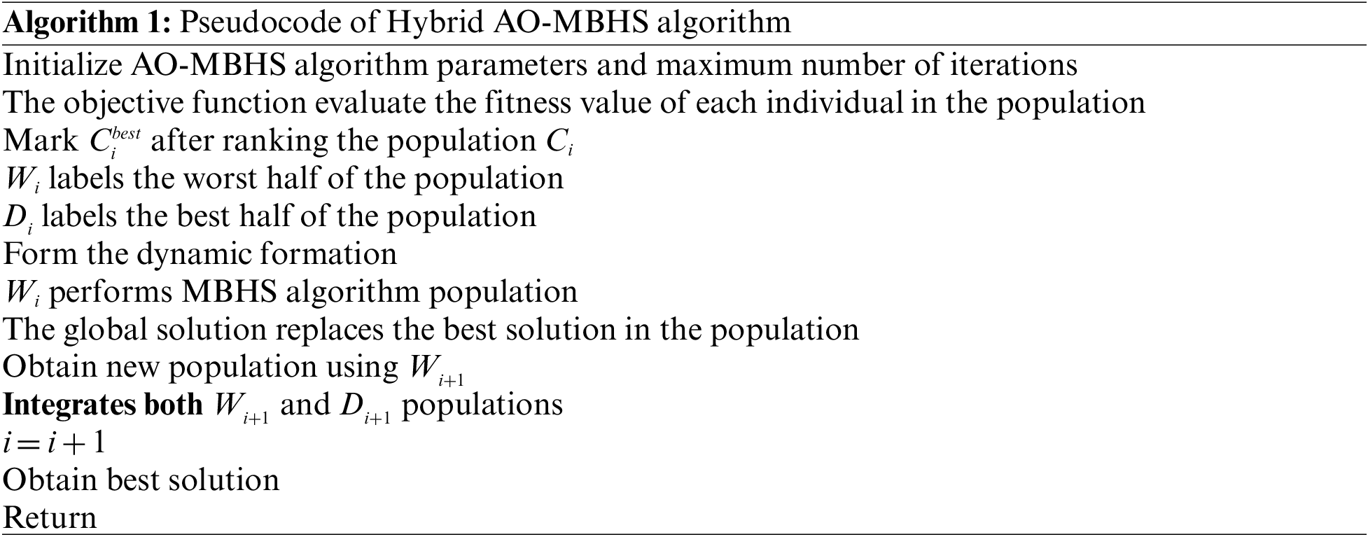
The proposed AO-MBHS algorithm integrates both the benefits (global searchability, fast convergence, etc.) of the AO and MBHS algorithm. To achieve this objective the AO and MBHS population is divided into two halves depending upon the fitness value of the individual. In the dynamic set formation, the population is divided into two halves based on the fitness value of each iteration. The AO algorithm is used to optimize the best half of the population and the MBHS algorithm is used to optimize the other half. The search operators with the same behavior may lead to the loss of diversity and this problem is overcome using the MBHS algorithm. Since the AO and MBHS algorithms parameters are different from each other, the AO-MBHS algorithm can enhance the capability of these algorithms by preventing them from being trapped in the local optima. In the search phase, the AO algorithm focuses on the local stage and the MBHS algorithm focuses on the global search. In this way, an efficient balance between the exploration and exploitation operators has been achieved. The MBHS algorithm uses the AO algorithm to optimize half of its population and to improve the convergence speed of the AO to lead to an easier convergence of the AO-MBHS algorithm. To the worst half of the population, the MBHS algorithm is applied to offer excellent exploration. This step prevents the worst half of the population from being trapped in locally optimal solutions and leads them to the global optimal solution. The AO-MBHS algorithm is formulated using the steps shown below:

Initialization Information: The parameters such as the maximum number of function evaluations, initial iteration i = 1, lower and upper boundaries of both algorithms, population size Psize, fitness function f(.), and problem dimensionality, etc. are taken as the initial parameters of the AO-MBHS algorithm. The current number of evaluations is set as 0 and the value of e is set as 1. Based on the initialized parameters, a random population is generated (Ci).

Population Evaluation: The fitness value of each individual in the population is computed depending upon the objective function which selects the optimal solution Cbest. The number of current function evaluations (FEcurrent) is computed using the below function

FEcurrent=FEcurrent+Psize(22)

End Condition: If the FEcurrent value is higher than the maximum number of function evaluations then the algorithm terminates or else it goes to the next step.

Dynamic Group Formation: The individuals in the population are mainly ranked based on their fitness values and after ranking the population Ci is marked as Cibest. The best half of the population is labeled as Di and the worst half of the population is labeled as Wi. These both populations can share their optimal solutions to enhance the convergence speed.

Optimizing the Population: The MBHS algorithm is performed for the population Wi. Initially, the best solution in the population is replaced with the global solution and the hyperparameters of the DCGAN architecture are ranked based on the fitness value. In the final step, the new population Wi+1 is obtained and the current number of function evaluations is updated using the equation shown below:

FEcurrent=FEcurrent+0.5∗Psize(23)

The AO algorithm is applied to the best half of the population Di. Every step in the AO algorithm is executed to get Di+1 population. In the optimization process of the AO algorithm, the fitness value of each individual is computed twice. Then the current number of function evaluations is obtained using the below equation:

FEcurrent=FEcurrent+Psize(24)

Population Integration: Both populations (Wi+1 and Di+1) are lastly integrated into Ci+1. The value of Bi is computed using Eq. (19) and the i value is updated using i = i + 1. Execute the end condition once. The flowchart of the hybrid AO-MBHS algorithm is presented in Fig. 1. Algorithm 1 explains the pseudocode of Hybrid AO-MBHS algorithm.

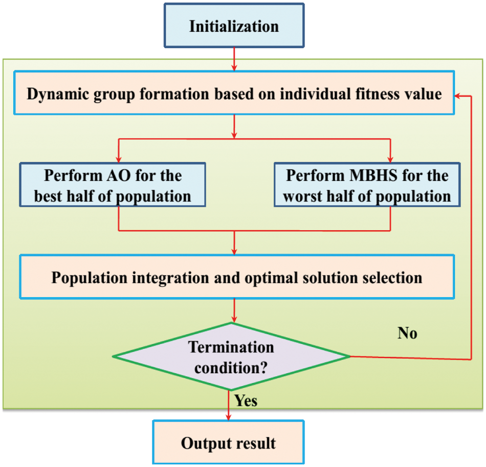
Figure 1: Flowchart of the hybrid AO-MBHS algorithm

3.3 Optimization of DCGAN Using Hybrid AO-MBHS Algorithm

The hyper parameters of DCGAN [9–12] are optimized in our work using the AO-MHBS algorithm which achieves a tradeoff between the exploration and exploitation stages. The GAN trains both the generator and discriminator in a simultaneous manner. The generator mainly takes an attack instance from the uniform distribution and generates the synthetic data very similar to that. The discriminator can correctly identify an actual attack and a synthetic attack and outputs the attack class accordingly. Using this strategy, the generator and discriminator play an adversarial role by modifying the DCGAN network weight and bias in each iteration. In this way, a synthetic attack is created which is similar to the actual attack. The AO-MBHS algorithm is mainly used to overcome different complexities associated with the DCGAN algorithm such as model collapse, instability, and vanishing gradients by tuning the DCGAN hyperparameters. The training algorithm used for the DCGAN is stochastic gradient descent with adam optimizer and the number of epochs used to train the adam optimizer is 2000. For a total of 70 epochs, the learning rate was taken as 0.002. The total number of search agents and iterations is set as 20. The batch size is 64 and the validation frequency is 1000. A sigmoid activation function is used as the discriminator. Using a zero centralized normal distribution with a B value of 0.02, the weight is initialized.

3.4 Novel Network Traffic Dataset Creation

The data is obtained from a real-time network which is utilized by different client organizations of varying sizes and mainly targeted towards different organizations. The network resembles a three-tier Internet Service Provider (ISP). This implies that the network receives the traffic generated by the client during network access and the reception of these requests by the conventional servers. Hence this network traffic generated helps to identify a wide range of user behavior. Many intrusion detection datasets focus on the traces collected from a certain university, coffee shops, malls, libraries, etc. The main features of the network are described as follows:

•   The internet access is provided via dual border routers namely R1 and R2. To analyze both the incoming and outgoing connections, a NetFlow probe is used.

•   Two different subnetworks are utilized by the ISP in which one is the main network and another one is an inner network of the organization. The firewall service is only provided to the systems present inside of the organization.

•   The attacker's network is present in the upper tier of the ISP where the five attacker machines are installed and they are numbered as X1–X5.

•   For dataset creation, we are deploying five victim systems in the core network which is connected with other clients in another network. This is known as the victim network (B1) and thesystems in this network are numbered from B11–B15.

•   In the internal infrastructure of the organization, an additional 15 victimized systems are placed and they are also interconnected with three different pre-existing networks. The pre-existing networks are equipped with five systems each. They are numbered as B2(B21–B25), B3(B31–B35), and B4(B41–B45).

3.4.1 Generation of Attack Traffic

When labeling real-time traffic we need to consider that the connections that are marked as attacks are really malicious or not. Hence we have integrated the real-time traffic that has attack traces with attacks that are generated for this experiment. To achieve this scenario, the victim systems are set with a similar ISP configuration used for the clients. The victim machines B1–B4 are set up to conduct attacks in the victim machines (Ba1–Ba5 and the value of a ranges from 1–4 at different time intervals). To prevent the attack obstruction by other neighboring ISPs and detection of the malicious behavior in the network both the victims and attackers are placed inside the network. The border router is selected as the place to deploy the attacker's network because it is where we can simulate the network traffic like it is generated from the internet.

3.4.2 Attack Deployment

In our work due to privacy reasons, we are not collecting the payload-related data and hence we do not include the attacks that are detectable by payload analysis. The two attack classes generated are synthetic and anomaly. The dos11, dos53s, dos53a, scan 11, scan 44, and botnet belong to the synthetic class, and the SPAM, UDP scan, and SSH scan belong to the anomaly class [21]. Fig. 2 presents the network topology of the attack generation scenario in detail. The network-related attacks taken in this work is described as follows:

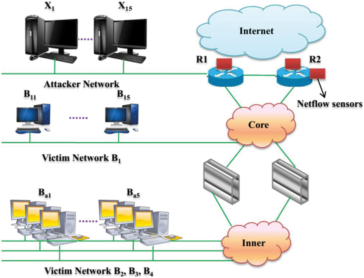
Figure 2: Attack creation scenario using the three-tier network topology

Low Rate Denial of Service Attacks

The Transmission Control Protocol (TCP) SYN packets are forwarded to the victims via the hping3 tool to combine the malicious traffic with the real world traffic the destination port is set as 80. Since this is a low-rate attack, the normal operations of the network are not affected. The different types of one to one DoS attack is delineated as follows:

One to one DoS attack: Here the attacker X1 attacks the victim B21 and the time duration of this attack is 3 min.

DoS53 synchronous: In this, the five attackers attack a total of three victims with a time period of 3 min. This attack has a specific structure such as (A1,A2)→B21, (A3,A4)→B31, and A5→B41. The DOS53 synchronous attacks imply that the attacks are conducted by the attackers at the same time.

DoS53-asynchronous: Here three attacks are conducted with a time period of 3 min sequentially and an inactivity period of 30 s is present in between three attacks. The total duration of this attack is 10 min.

Port Scanning

A SYN scan is run continuously for 3 min to scan the common ports of the victims for 3 min using the nmap tool. Scan 11 (one to one scan attack) and scan44 (four to four scan attacks) are the two types of port scanning attacks conducted. The scan11 attack is carried in sequence while the scan44 attack is conducted in parallel.

Botnet Traffic

The botnet attacks are quite popular these days and hence a botnet attack is included in our work. Since we are not capable of handling the issues caused by the botnet attack in an open network, we are mixing the botnet traces obtained in a controlled environment with our network traffic. The attack created in this way is not fully realistic but it somewhat replicates the effect of the botnet attack.

UDP Scan Attack

This attack takes place in a short time with an increase of Acknowledgement (ACK) packets with the UDP connection. Each victim in the network is scanned with a specific range of 60 ports based on the source port of the connection.

Secure Socket Shell (SSH) Scan Attack

It originates with an increase in the SSH traffic generated by a single machine hosted in the Internet Service Provided.

SPAM Attack

To retrieve sensitive information from the users, this attack is conducted by sending a huge amount of unsolicited messages via instant messaging applications. This type of attack traffic is found in both the normal and attack sets.

3.5 DCGAN Architecture for Adversarial Malware Generation

Since a large labeled training dataset is needed to train the DCGAN network [22], we generated new samples using a generative model. The synthetic traffic generated is tested via a black box detector equipped with AI-based algorithms. We can get the results for our synthetic dataset from the black box detector. The adversarial instances probability distribution is identified by the weights of the generator. To enhance the AI-based black box detector's efficiency, the samples in the test and training set follow the same probability distribution. The generator makes variations in the probability distribution of the malware instances present in both the testing and training dataset to confuse the black box detector. In this way, the generator confuses the AI-based BlackBox classifier's efficiency. The outline of the model is shown in Fig. 3.

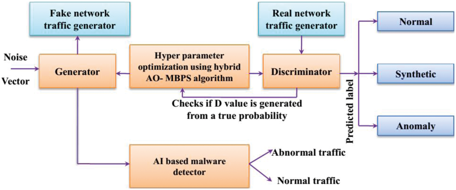
Figure 3: Outline of the proposed model

GAN is a generative model and it implicitly learns the data distribution (A) from a set of samples y(1),…,y(n) to create new samples from the learned distribution. In this paper, we have used a deep convolutional GAN architecture and both the generator and discriminator follow a DCNN architecture and it also acts as an AI-based malware detector. This model is formed by concatenating two neural networks trained concurrently. In this study, the novelty of the discriminator (D) network is to identify the difference between the real and synthesized network traffic. It is provided an input a and it outputs D(a) which is termed as the probability of the actual sample. G is the name of the Generator network, and it creates samples to deceive D into believing it is agenuine sample with a high probability value. The generator receives samples x(1),…,x(n) from a known sample distribution (px). The main aim of G is to retrieve the value of A. The following loss function needs to be optimized to create the adversarial network.

minG⁡maxD⁡Ey∼Alog⁡D(y)+Ey∼px[log⁡(1−D(G(x)))](25)

The discriminator's main aim is to increase the D(y) value of instances for y∼A and to decrease D(y) for y≠A. The generator generates malicious samples G(y) to fool the detector during the training process in which D(G(x))∼A. The generator is either trained to minimize D(G(x)) or maximize 1−D(G(x)). In the training process, the generator enhances its capability to generate more realistic samples and the discriminator enhances its capability to identify the difference between the actual and synthesized samples. The generator changes the malware feature vector into its adversarial version. It integrates both the noise vector (v) and malware features as input. Every element present in the vector v describes an absence or presence of the feature. The outline of the proposed methodology is presented in Fig. 3 and it is self-explanatory. Finally, the discriminator predicts normal, synthetic and anomalies.

4  Experimental Analysis and Results

The real intrusion network traffics similar to the synthetic intrusion network traffic of high quality. The detection rate is determined via model measurement as accuracy. The evaluation measures including accuracy (A), negative predictive value (NPV), positive predictive value (PPV), detection rate (DR), Recall, Precision, F-Score, and false alarm rate (FAR) are explained in this section. Accuracy is defined as the total number of correctly classified samples to the total number of samples tested. Recall can be defined as the total number of correctly classified positive data to the total number of positive data in the testing samples. Precision is the ratio of correctly classified positive data to the total number of positive data. F-score is defined as the weighted average of precision and recall.

The proposed method detects the attack instances ratio signified using detection rate (DR). The misclassified normal instances ratio is signified using a false alarm rate (FAR). The proposed method performance is superior in terms of decreasing FAR with increasing DR. Tab. 1 express the hyperparameter settings of proposed method.

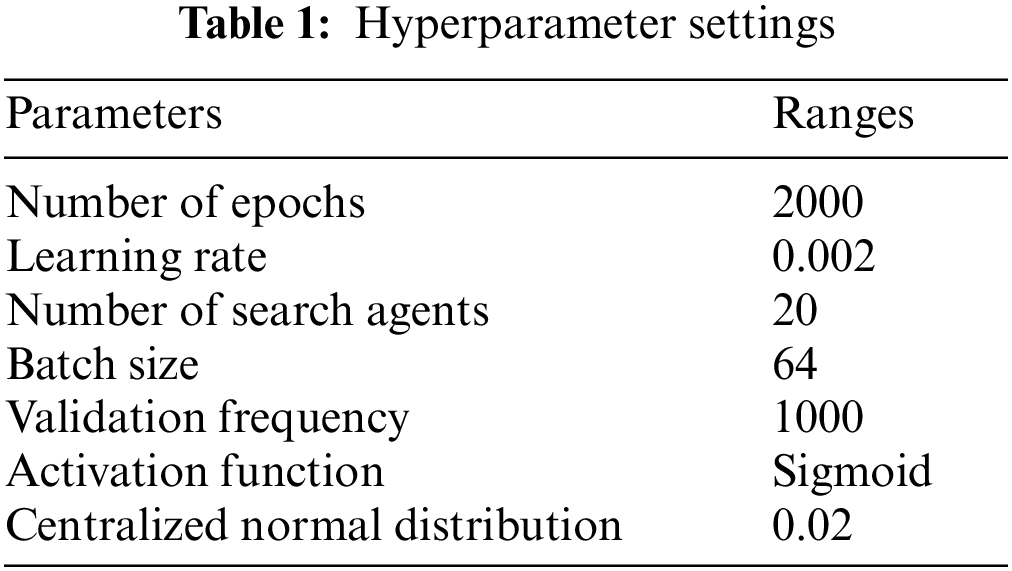
Fig. 4 describes the training progress of the DGCAN based AOA MBHA with respect to accuracy and loss function as described in Figs. 4a and 4b. The proposed model is trained by using seventy percentages of data and the remaining 30% is used for the testing process. Fig. 4a describes the training progress of DGCAN based AOA MBHA accuracy curve. The training progress of DGCAN based AOA MBHA loss function curve is plotted in Fig. 4a. In all epochs, we discovered minimum loss with superior accuracy by using the proposed method as shown in Fig. 4.

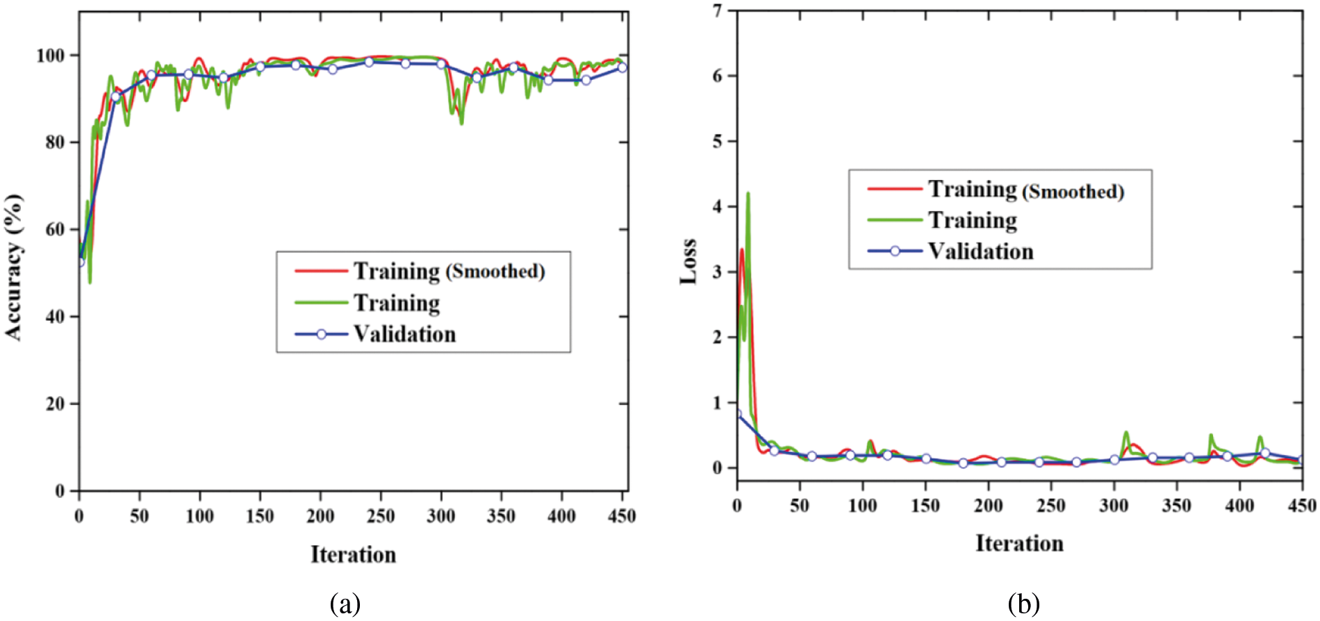
Figure 4: Training progress of the DGCAN based AOA MBHA, (a) Accuracy and (b) Loss

Fig. 5 describes the Receiver Operating Characteristic (ROC) curve results of the proposed method in attack generation. After each of four adversarial rounds, the ROC curve of the proposed model is plotted based on 10 folds cross-validation. After three rounds, the apparent asymptote with the number of adversarial rounds degrades the performance due to GAN generates confusion. The DGA detector performance is improved using the proposed method. After three rounds, the adversarial rounds are based on all the subsequent experiments.

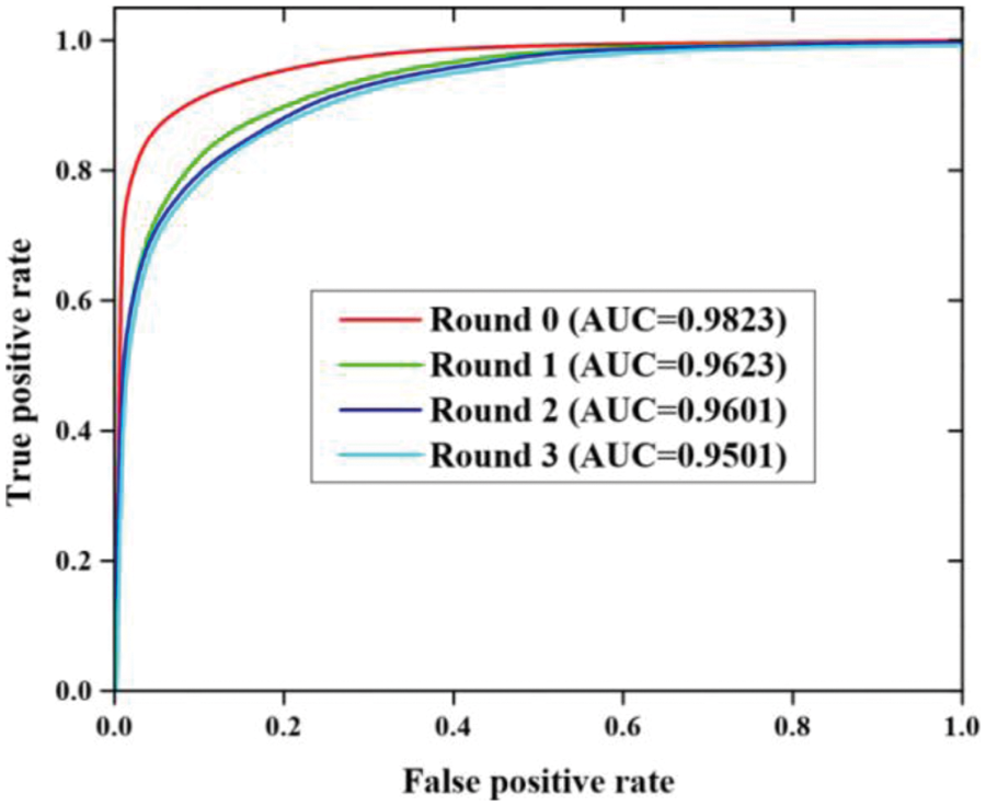
Figure 5: ROC curve results of proposed work

The experimental result of cross-validation is described in Fig. 6. The data is divided into k times for both training and testing in which an important instrument to predicting network performance is cross-validation. The proposed work performance is validated over ten iterations (k = 10) in the present work. The k and k- subsets1is are used for both training and testing procedures. Calculate the error rate.

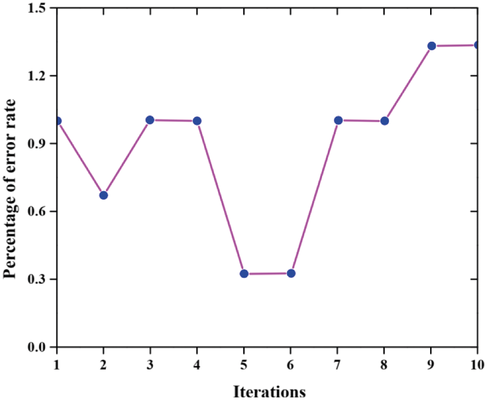
Figure 6: Experimental result of cross-validation

The different learning rate with loss function value is depicted in Fig. 7. When the learning rate is 0.01, 0.001, and 0.0001 values that compared the loss function in order to validate the effect of epoch number on the proposed technique. This graph is plotted between the number of iterations and the resultant dependency of loss functions. The number of iterations is represented in the X coordinate and the loss function value is represented using the Y coordinate. This investigation consists of 100 to 1000 iterations.

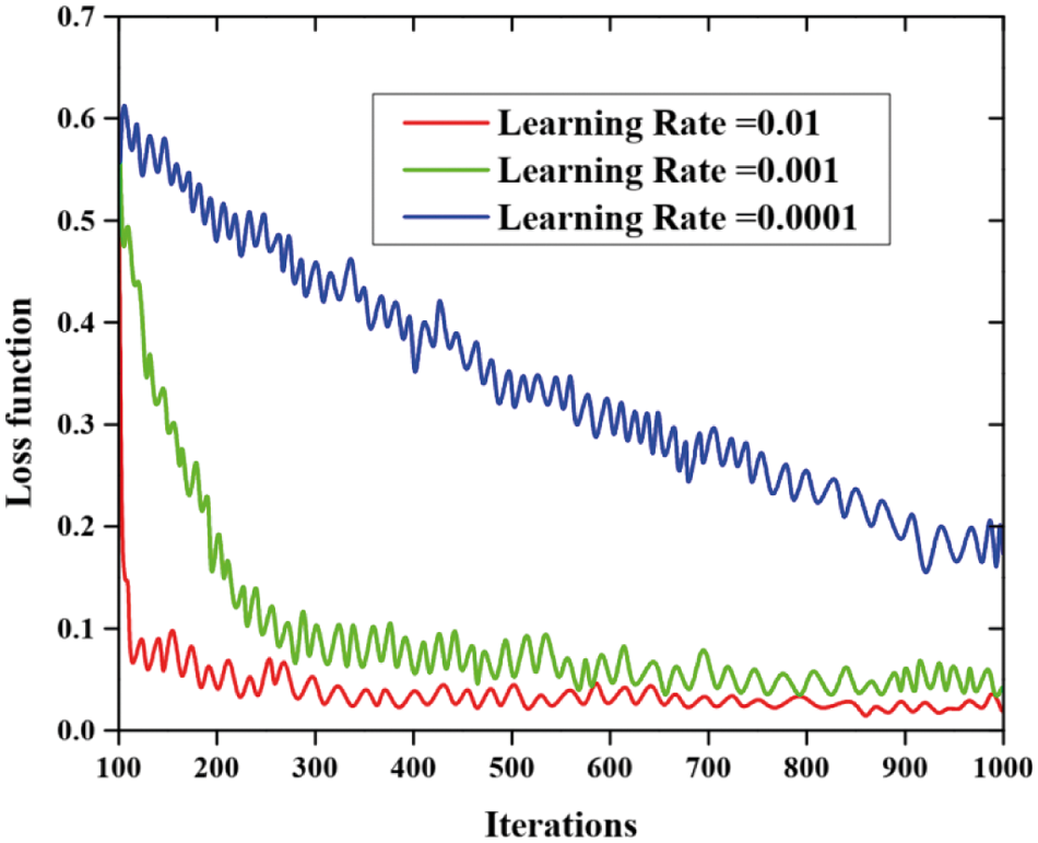
Figure 7: Different learning rate with the loss function value

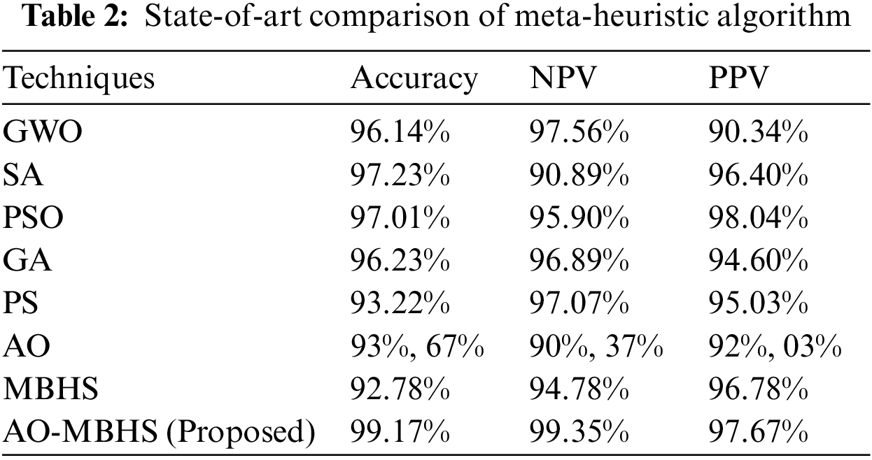
Tab. 2 describes the state-of-art comparison of the meta-heuristic algorithm. This investigation is carried out among the measures such as accuracy, NPV, and PPV with the pattern search (PS) [22], genetic algorithm (GA) [23], simulated annealing (SA) [24], particle swarm optimization (PSO) [25], Grey Wolf Optimization (GWO) [26] and proposed algorithm. The proposed algorithm provides superior results such as 99.17% accuracy, 99.35% NPV, and 97.67% PPV results.

4.1 Detection Analysis

To analyze the performance of the proposed DCGAN based AO-MBHS based approach we have deemed a maximum number of ground-truth information. To compare the performance we have taken the DCGAN approach. The comparative analysis is depicted in Fig. 8.

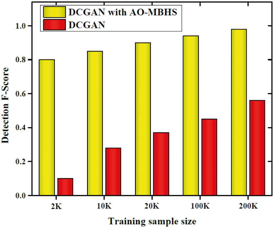
Figure 8: Detection analysis F-score

Fig. 9 shows the attack detection performance of proposed and DCGAN approaches for up to 200 K samples. The proposed method shows a better detection F-score than the DCGAN. For 200 k samples, the detection F-Score of the proposed method is almost equal to 0.9923 and the DCGAN shows a 0.5609 F-score. Thus our method performs well for maximum ground-truth information.

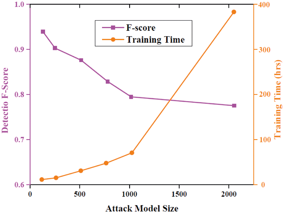
Figure 9: Performance analysis of detection of attacks created by various methods along with their training costs

4.2 Training Loss Analysis

The tradeoff that occurs between the F-score and increasing training time of the attacker are illustrated in Fig. 9. The F-score has been decreased with the training of larger methods. When the training size increases from 128 to 256 then the performance dropped greatly. Thus the increase in method size will increase the computational complexity.

The training loss of six models including 3 plain models and 3 residual models are analyzed and plotted in Fig. 10. The training loss of residual blocks is small since it will represent the network degradation issues. From the Fig. 10, it is evident that the training loss values decreased continuously with the training process increases. From the figure when the epoch reached 20 the training loss decreases sharply.

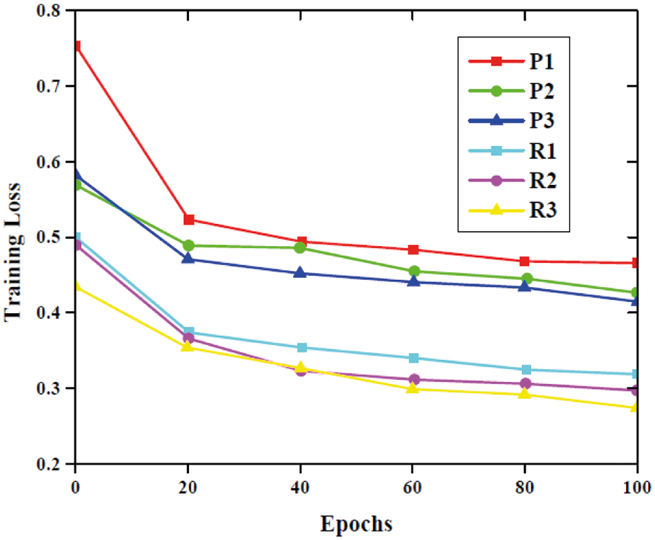
Figure 10: Performance analysis based on training loss

4.3 Classification of Attacks Analysis

The detection of proposed work can be evaluated by considering the attacks such as DoS11, DoS53s, DoS53a, Scan11, Scan44, Botnet, IP in Blacklist, UDP Scan, SSH Scan, SPAM with the existing works such as SVM [27], MLP [28], Faster RCNN [29], CNN [30], and DCGAN approaches [31]. Fig. 11 shows the recall values of all the classifiers that have been taken. Our proposed method shows better classification due to the higher recall values. The recall values depend on the type of attacks and for minor attackers the recall value is low for all types of classifiers and major attacks the recall value is high and our proposed method exhibits better classification outcomes.

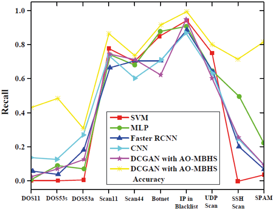
Figure 11: Classification of attacks based on the recall and accuracy

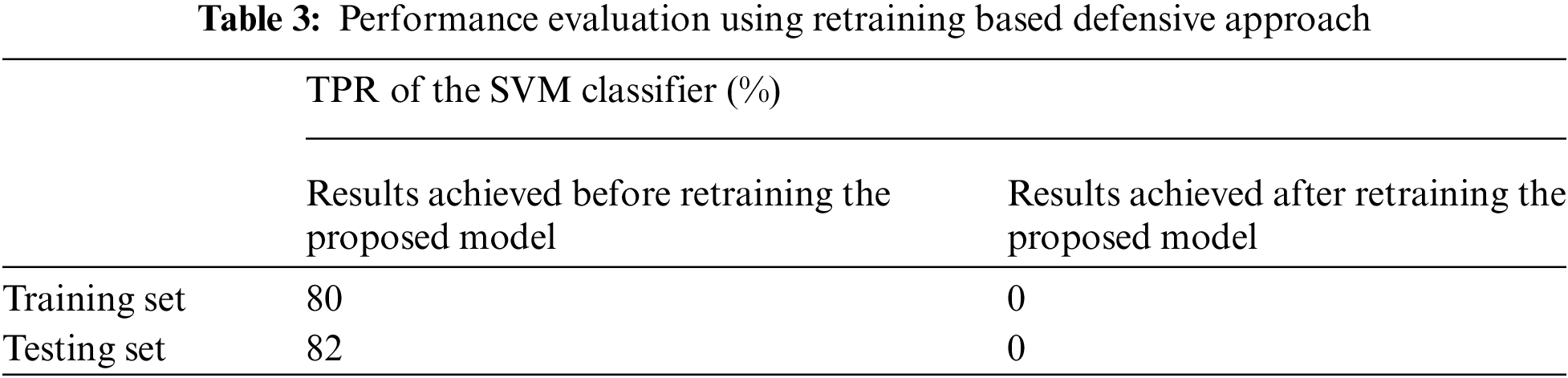
4.4 Performance Evaluation Using Retraining Based Defensive Approach

The performance of the proposed model is evaluated using the retraining-based defensive approach in this section. Using our new dataset created the SVM classifier [32] is trained using the adversarial samples to detect the presence of a malicious entity. Before retraining the proposed classifier, the SVM classifier [33] is able to classify 80% of samples but after retraining the proposed hybrid AO-MBHS optimized DCGAN classifier, the SVM classifier can barely recognize any adversarial instances. The results obtained are demonstrated using Tab. 3. The TPR of the SVM classifier is reduced from 80% to 0% in a single epoch of retraining the proposed model. The proposed model is run a total of ten times and the result is the same for all.

5  Conclusion

The paper presents a hybrid AO-MBHS based DGCA model to generate network traffic instances that are undetected by the AI-based malware detector algorithms. The AI-based malicious detectors act as malware detectors. The malware network traffic is generated via the generator equipped with a DCNN architecture which fools the detector in discriminating the samples. Real-time network traffic that has attack traces is used in the experiment using an ISP configuration by placing both the attackers and victims inside the network. To identify the malicious content generated by the dataset, the intrusion detection system developers need to construct a large dataset with enough adversarial traffic. But this process is time-consuming and labeling them is a manually intensive task. The SVM is used as the malicious traffic detection application and its TPR rate goes from 80% to 0% after retraining the proposed model which shows the efficiency of the proposed model in hiding the samples. When trained with different performance metrics, the proposed methodology provides efficient F-Score, low loss rate, higher accuracy, and higher NPV and PPV values. The percentage of error rate is low even during cross-validation and the proposed methodology also shows high ROC values in generating the attacks.

Funding Statement: This project was funded by the Deanship of Scientific Research (DSR) at King Abdulaziz University, Jeddah, under Grant No. RG-91-611-42. The authors, therefore, acknowledge with thanks to DSR technical and financial support.

Conflicts of Interest: The authors declare that they have no conflicts of interest to report regarding the present study.

References

 1.  Z. Lina, Y. Xiao and W. Chen, “Vulnerability to machine learning attacks of optical encryption based on diffractive imaging,” Optics and Lasers in Engineering, vol. 125, pp. 105858–105865, 2020. [Google Scholar]

 2.  M. Alloghani, A. J. Dhiya, A. Hussain, J. Mustafina, T. Baker et al., “Implementation of machine learning and data mining to improve cybersecurity and limit vulnerabilities to cyber-attacks,” in Nature-Inspired Computation in Data Mining and Machine Learning, Cham: Springer, pp. 47–76, 2020. [Google Scholar]

 3.  H. R. Hung, M. C. Peng, C. W. Huang, P. C. Lin, V. L. Nguyen et al., “An unsupervised deep learning model for early network traffic anomaly detection,” IEEE Access, vol. 8, pp. 30387–30399, 2020. [Google Scholar]

 4.  D. Spiekermann and J. Keller, “Unsupervised packet-based anomaly detection in virtual networks, ”Computer Networks, vol. 192, pp. 108017–108026, 2021. [Google Scholar]

 5.  C. Pontes, M. Souza, J. Gondim, M. Bishop, M. Marotta et al., “A new method for flow-based network intrusion detection using the inverse potts model,” IEEE Transactions on Network and Service Management, vol. 18, no. 2, pp. 1125–1136, 2021. [Google Scholar]

 6.  S. Sriram, R. Vinayakumar, M. Alazab and K. P. Soman, “Network flow based IoT botnet attack detection using deep learning,” in IEEE INFOCOM 2020-IEEE Conf. on Computer Communications Workshops, Toronto, Canada, IEEE, pp. 189–194, 2020. [Google Scholar]

 7.  S. Zavrak and M. Iskefiyeli, “Anomaly-based intrusion detection from network flow features using variational autoencoder,” IEEE Access, vol. 8, pp. 108346–108358, 2020. [Google Scholar]

 8.  M. R. Rejeesh, “Interest point based face recognition using adaptive neuro fuzzy inference system,” Multimedia Tools and Applications, vol. 78, pp. 22691–22710, 2019. [Google Scholar]

 9.  M. Ring, D. Schlör, D. Landes and A. Hotho, “Flow-based network traffic generation using generative adversarial networks,” Computers & Security, vol. 82, pp. 156–172, 2019. [Google Scholar]

10. M. Kawai, K. Ota and M. Dong, “Improved malgan: Avoiding malware detector by leaning cleanware features,” in 2019 Int. Conf. on Artificial Intelligence in Information and Communication (ICAIIC), Okinawa, Japan, IEEE, pp. 40–45, 2019. [Google Scholar]

11. W. Hu and Y. Tan, “Generating adversarial malware examples for black-box attacks based on GAN,” arXiv preprint arXiv:1702.05983, pp. 1–7, 2017. [Google Scholar]

12. M. F. Adar, I. Diamant, E. Klang, M. Amitai, J. Goldberger et al., “GAN-based synthetic medical image augmentation for increased CNN performance in liver lesion classification,” Neurocomputing, vol. 321, pp. 321–331, 2018. [Google Scholar]

13. A. S. Hyrum, J. Woodbridge and B. Filar, “DeepDGA: Adversarially-tuned domain generation and detection,” in Proc. of the 2016 ACM Workshop on Artificial Intelligence and Security, Vienna Austria, pp. 13–21, 2016. [Google Scholar]

14. M. Mahrishi, S. Morwal, A. W. Muzaffar, S. Bhatia, P. Dadheech et al., “Video index point detection and extraction framework using custom yolov4 darknet object detection model,” IEEE Access, vol. 9, pp. 143378–143391, 2021. [Google Scholar]

15. R. Singla, N. Kaur, D. Koundal, S. A. Lashari, S. Bhatia et al., “Optimized energy efficient secure routing protocol for wireless body area network,” IEEE Access, vol. 9, pp. 116745–116759, 2021. [Google Scholar]

16. L. Abualigah, D. Yousri, M. A. Elaziz, A. A. Ewees, M. A. A. Al-Qaness et al., “Aquila optimizer: A novel meta-heuristic optimization algorithm,” Computers & Industrial Engineering, vol. 157, pp. 107250–107264, 2021. [Google Scholar]

17. A. Sadollah, H. Sayyaadi, H. M. Lee and J. H. Kim, “Mine blast harmony search: A new hybrid optimization method for improving exploration and exploitation capabilities,” Applied Soft Computing, vol. 68, pp. 548–564, 2018. [Google Scholar]

18. A. Sadollah, H. M. Lee and J. H. Kim, “Mine blast harmony search and its applications,” in Harmony Search Algorithm, Berlin, Heidelberg: Springer, pp. 155–168, 2016. [Google Scholar]

19. D. Markovi and G. Petrovi, “Assessing the performance of improved harmony search algorithm (IHSA) for the optimization of unconstrained functions using taguchi experimental design,” Scientific Research and Essays, vol. 7, no. 12, pp. 1312–1318, 2012. [Google Scholar]

20. Z. W. Geem and K. B. Sim, “Parameter-setting-free harmony search algorithm,” Applied Mathematics and Computation, vol. 217, no. 8, pp. 3881–3889, 2010. [Google Scholar]

21. G. Maciá-Fernández, J. Camacho, R. Magán-Carrión, P. García-Teodoro, R. Therón et al., “UGR ‘16: A new dataset for the evaluation of cyclostationarity-based network IDSs,” Computers & Security, vol. 73, pp. 411–424, 2018. [Google Scholar]

22. R. Hooke and T. A. Jeeves, “Direct search solution of numerical and statistical problems,” Journal of ACM, vol. 8, no. 2, pp. 212–29, 1961. [Google Scholar]

23. J. H. Holland, “Genetic algorithms, “Scientific American, vol. 267, no. 1, pp. 66–72, 1992. [Google Scholar]

24. P. J. V. Laarhoven and E. H. Aarts, “Simulated annealing. In simulated annealing: Theory and applications,” in Mathematics and its Applications, Reidel, Dordrecht; Boston: D. Reidel; Norwell, MA, U.S.A.: Sold and distributed in the U.S.A. and Canada by Kluwer Academic Publishers, pp. 7–15, 1987. [Google Scholar]

25. M. R. Rejeesh and P. Thejaswini, “Multi-objective optimal trilateral filtering based partial moving frame algorithm for image denoising,” Multimedia Tools and Applications, vol. 79, pp. 28411–28430, 2020. [Google Scholar]

26. S. M. Mirjalili and A. Lewis, “Grey wolf optimizer,” Advances in Engineering Software, vol. 69, pp. 46–61, 2014. [Google Scholar]

27. O. Bamasaq, D. Alghazzawi, S. Bhatia, P. Dadheech, F. Arslan et al., “Distance matrix and markov chain based sensor localization in wsn,” Computers, Materials and Continua, vol. 71, no. 2, pp. 4051–4068, 2022. [Google Scholar]

28. R. Pahuja and A. Kumar, “Sound-spectrogram based automatic bird species recognition using MLP classifier,” Applied Acoustics, vol. 180, pp. 108077–109090, 2020. [Google Scholar]

29. X. Mai, H. Zhang, X. Jia and M. Q. H. Meng, “Faster R-CNN with classifier fusion for automatic detection of small fruits,” IEEE Transactions on Automation Science and Engineering, vol. 17, no. 3, pp. 1555–1569, 2020. [Google Scholar]

30. M. Piekarczyk, O. Bar, L. Bibrzycki, M. Niedźwiecki, K. Rzeck et al., “CNN-based classifier as an offline trigger for the credo experiment,” Sensors, vol. 21, no. 14, pp. 4804–4820, 2021. [Google Scholar]

31. D. Alghazzawi, O. Bamasaq, S. Bhatia, A. Kumar, P. Dadheech et al., “Congestion control in cognitive iot-based wsn network for smart agriculture,” IEEE Access, vol. 9, pp. 151401–151420, 2021. [Google Scholar]

32. S. S. Kshatri, D. Singh, B. Narain, S. Bhatia, M. T. Quasim et al., “An empirical analysis of machine learning algorithms for crime prediction using stacked generalization: An ensemble approach,” IEEE Access, vol. 9, pp. 67488–67500, 2021. [Google Scholar]

33. S. H. Kok, A. Abdullah, N. Z. Jhanjhi and M. Supramaniam, “A review of intrusion detection system using machine learning approach,” International Journal of Engineering Research and Technology, vol. 12, no. 1, pp. 8–15, 2019. [Google Scholar]

This work is licensed under a Creative Commons Attribution 4.0 International License, which permits unrestricted use, distribution, and reproduction in any medium, provided the original work is properly cited.