Computers, Materials & Continua DOI:10.32604/cmc.2022.025339
Article

Effective Classification of Synovial Sarcoma Cancer Using Structure Features and Support Vectors

P. Arunachalam1, N. Janakiraman1, Junaid Rashid2, Jungeun Kim2,*, Sovan Samanta3, Usman Naseem4, Arun Kumar Sivaraman5 and A. Balasundaram6

1Department of Electronics and Communication Engineering, K.L.N. College of Engineering, Pottapalayam, 630612, Tamil Nadu, India
2Department of Computer Science and Engineering, Kongju National University, Cheonan 31080, Korea
3Department of Mathematics, Tamralipta Mahavidyalaya, Tamluk, 721636, West Bengal
4School of Computer Science, University of Sydney, NSW 2006, Australia
5School of Computer Science and Engineering, Vellore Institute of Technology, Chennai, 600127, India
6School of Computer Science and Engineering, Centre for Cyber Physical Systems, Vellore Institute of Technology, Chennai, 600127, India
*Corresponding Author: Jungeun Kim. Email: jekim@kongju.ac.kr
Received: 20 November 2021; Accepted: 06 January 2022

Abstract: In this research work, we proposed a medical image analysis framework with two separate releases whether or not Synovial Sarcoma (SS) is the cell structure for cancer. Within this framework the histopathology images are decomposed into a third-level sub-band using a two-dimensional Discrete Wavelet Transform. Subsequently, the structure features (SFs) such as Principal Components Analysis (PCA), Independent Components Analysis (ICA) and Linear Discriminant Analysis (LDA) were extracted from this sub-band image representation with the distribution of wavelet coefficients. These SFs are used as inputs of the Support Vector Machine (SVM) classifier. Also, classification of PCA + SVM, ICA + SVM, and LDA + SVM with Radial Basis Function (RBF) kernel the efficiency of the process is differentiated and compared with the best classification results. Furthermore, data collected on the internet from various histopathological centres via the Internet of Things (IoT) are stored and shared on blockchain technology across a wide range of image distribution across secure data IoT devices. Due to this, the minimum and maximum values of the kernel parameter are adjusted and updated periodically for the purpose of industrial application in device calibration. Consequently, these resolutions are presented with an excellent example of a technique for training and testing the cancer cell structure prognosis methods in spindle shaped cell (SSC) histopathological imaging databases. The performance characteristics of cross-validation are evaluated with the help of the receiver operating characteristics (ROC) curve, and significant differences in classification performance between the techniques are analyzed. The combination of LDA + SVM technique has been proven to be essential for intelligent SS cancer detection in the future, and it offers excellent classification accuracy, sensitivity, specificity.

Keywords: Principal components analysis; independent components analysis; linear discriminant analysis; support vector machine; blockchain technology; IoT application; industry application

1  Introduction

The medical industrial applications are one of the fastest growing industries in the world for diagnosing diseases with the help of IoT applications through blockchain techniques to protect patients from harmful chronic diseases. Recently, digital clinical histopathology images have proposed numerous cancer cell classification techniques for brain, breast, cervical, liver, lung, prostate and colon cancers [1]. A synovial sarcoma (SS) is a mesenchymal tissue cell tumour that most frequently occur commonly in the limb of adolescents and young adults [2]. The SS peak incidence is observed in the most common in children and adolescents younger than 20 years of age, the annual occurrence rate is 0.5 to 0.7 per million [3]. SS has a variety of morphological patterns, but its chief forms are the monophasic and biphasic spindle cell patterns [4]. These two types of spindle cells appear looking like an ovoid shape are called as spindle shaped cell (SSC), as shown in Fig. 1 [5,6].

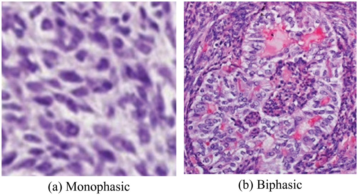
Figure 1: The SS cancer images and their SSC (oval-shape) structure of the components

The digital histopathological examination is a crucial technique for diagnosis, but it is still not established in cancer cell structures often non-specific, it overcomes through wavelet transform (WT) has too often been helpful. The WT has transformed into sub-band image and it consists of the resolution scale wavelet coefficients and set of detail sub-band orientation. Hence, the sub-band image such as discrete wavelet transform (DWT) analysis are necessary to address the different behaviour of cell structure in order to describe it as an image [7]. Moreover, the DWT is well suitable to calculate cell structure pixel intensity value of an image. WT is a very powerful mathematical tool similar to the signal processing technique compared to the Fourier Transform (FT) and is used in various medical imaging applications [8]. Wavelet, which is used at different scales to decompose a signal, provides better resolution characteristics for WT in the 1D and 2D versions of the time scale plane [9]. WT decomposes an image approximation, the detail coefficients of which operate first with 1D wavelets and finally with columns. The result is that the first level of 2D DWT is calculated as an image. The images here are decomposed by low and high pass filters to obtain approximate (LL or A1), horizontal (LH or H1), vertical (HL or V1) and diagonal (HH or D1) coefficients [10]. Further, the first level approximation (A1) coefficients sub-band image is decomposed into three level wavelet coefficients, from this the structural features of the wavelet coefficients (Haar wavelet) are extracted and used to differentiate the cell structure by support vectors (SVs) [11].

Most of the studies on cancer classification have been achieved through the use of supervised or unsupervised pixel-wise classification of small rectangular image regions in terms of color and texture [12]. Similarly, for data classification, decisions are made based on a set of features. Here, many structural or pattern authentication tasks are first used by the pathologist, and then the same features are used in the automated classification [13,14]. However, it can also be a difficult task. Fortunately, pathologist does not have to use the features used in machines. Assessing to pathologists, sometimes difficult features are easily extracted and used in automated systems.

Thiran et al. [15] proposed a mathematical morphological technique. This technique first removes the noise behind the image and analyzes its size, shape and texture. Subsequently, the image is classified as cancer or normal based on the extracted values. Smith et al. [16] have proposed similarity measurement method for the classification of architecturally differentiated image sections is described prostate cancer. In this application, the Fourier transform and eigenvalue based method is recommended for the Gleason grading of histology slide images of prostate cancer. Khouzani et al. [7] have presented that the classification of image grade is proposed by two perspectives. First, the entropy and energy features are derived from the multiwavelet coefficients of the image. Then, to categorize each image to the appropriate quality, the simulated annealing algorithm and the k-nearest neighbor (k-NN) classifier select the most discriminating features. Second, wavelet packets and co-occurrence matrixes features are extracted. Then, they are compared to the multiwavelet method. The testing shows superiority of multiwavelet transformations compared to other methods. For multivariable, critically sampled pre-processing improves back-to-front pre-processing and is less sensitive to the noise of second-level decomposition. Most researchers do not use it in extraction because it is more sensitive to first-level noise.

Huang et al. [17] have extracted intensity and co-occurrence (CO) features such as intensity, morphology, and texture features from the separated nuclei in the images. It has been effectively differentiated varying degrees of malignancy and benignity by applying local and global characteristics. The SVM based decision map classifier with feature subset selection is used for each endpoint of the classifier compared to the k-NN and SVM model. The accuracy rate of the classification is increased by 1.67% with the SVM based decision graph classification. Doyal et al. [18] have presented a boosted Bayesian multiresolution (BBMR) system to identify regions of prostate cancer (CaP) in digital biopsy slides. They extracted image features such as first-order statistical, second-order co-occurrence, and Gabor filter features using the AdaBoost ensemble method. The BBMR approach has been found to have higher values of accuracy and area under the receiver operating characteristics (AUROC) curve than the other classifiers using the random forest feature ensemble strategy. Al-Kadi [19] has represented a multiresolution analysis technique based on wavelet packets and fractal dimensions (FD) for brain tumor meningioma classification. WT has applied the morphological process to blue color channel images. The wavelet sub-bands with high FD signatures are selected and used for classification in SVM, naive Bayesian and the k-NN classifier. The SVM classifier achieves better performance characteristics of the energy-texture signatures selection approach compared to the co-occurrence matrix signatures.

Ding et al. [20] have introduced three types of features for SVM classification, namely monofractal, multifractal, and Gabor features, which can be used to efficiently separate microbial cells from histological images and analyze their morphology. Their experiments show that the proposed automated image analysis framework is accurate and scalable to large data sets. Spanhol et al. [21] were introduced to estimate six different texture descriptors in different classifiers, and reported that the accuracy ranges rates of 80% to 85%, depending on different image magnification factors. There is no denying that texture descriptors provide a good representation of classification training. However, some researchers advise that the main weakness of current machine learning methods is the ability to learn representatives. Features extraction methods play an important role in the malignancy classification of histopathology image. Histopathological images of different cancer types have dramatically different color, morphology, size, and texture distributions. It is difficult to identify the common structures of malignancy diagnosis that can be used for the classification of colon and brain cancer. Therefore, features extraction [22] is very important in the high-level histopathology image task of classification. Kong et al. [23] used a similar multiresolution framework for grading neuroblastoma in the pathological image. They demonstrated that the subsets of features obtained by sequential floating forward selection are subject to dimension reduction. The tissue regions are hierarchically classified by using k-NN, LDA + nearest mean (NM), LDA + k-NN, correlation LDA + NM, LDA + Bayesian and SVM with a linear kernel. Classification accuracy is achieved by the SVM classifier due to the selected optimal subset of features.

In this work, the application of blockchain technology based IoT devices to classify SS cancer through a combined study of SF and SVM methods leads to access to a wide range of secure histopathological imaging data for processing multiple histopathological imaging data within the cancer classification. Blockchain is an information base, or record that is shared across an organizational network. This record is encoded to such an extent that solitary approved parties can get to the information. Since the information is shared, the records can't be altered. Rather than transferring our information on a brought together cloud, we appropriate across an organization over the world. Blockchain-based distributed storage consummately joins security and versatility with its interlinked blocks, hashing capacities, and decentralized design. It settles on the innovation an optimal decision for adding an additional layer of safety to the distributed storage. So, the security components intrinsic of blockchain can be supported utilizing the logical force of profound deep learning and Artificial Intelligence.

In the domain of sharing of SS image information, the capacity to safely and effectively measure monstrous measures of information can create a huge incentive for organizations and end-clients. Simultaneously, the IoT empowered gadgets across the Internet to send information to private blockchain organizations to make, alter safe records of shared SS image information. For instance, IBM Blockchain empowers our establishment accomplices to share and access IoT information without the requirement for focal control and the board. Each sharing can be confirmed to forestall questions and construct trust among all permissioned network individuals. SVs for SF stored on IoT devices are trained with a large number of distributed high-quality image data [24,25].

Spindle Shaped cells (SSC) are specialized cells that are longer than they are wide. They are found both in normal, healthy tissue and in tumors. The proposed approach used dimensionality reduction techniques to extract structure features (SFs) from third-level Haar wavelet sub-band images as follows: (1) Principal Component Analysis (PCA) gives second order statistical pixel variance, (2) Independent Components Analysis (ICA) gives higher order statistical to extract independent component pixel variance, and (3) Linear Discriminant Analysis (LDA) gives optimal transformation by minimizing the within-class and maximizing the between-class distance simultaneously (co-variance pixel value). Therefore, storing and sharing histopathological image data through a decentralized and secure IoT network can lead to in-depth learning from various histopathological image health care centres and medical industry [26]. Moreover, this work used dimensionality reduction techniques to extract structure features (SFs) from third-level Haar wavelet sub-band images as follows: (1) Principal Component Analysis (PCA) gives second order statistical pixel variance, (2) Independent Components Analysis (ICA) gives higher order statistical to extract independent component pixel variance, and (3) Linear Discriminant Analysis (LDA) gives optimal transformation by minimizing the within-class and maximizing the between-class distance simultaneously (co-variance pixel value) [27,28]. Therefore, these dimensionality reduction techniques are implemented before classifiers are trained. As a result, the complexity of Support Vector Machine (SVM) classifier is reduced, convergence velocity and performance of classifier has increased. Hence, SVM is used to find the optimal hyperplane to separate different class mapping input data into high dimensional feature space [29]. Furthermore, this work chosen the Radial Basis Function (RBF) kernel [30] and their tuning parameters to train these extracted SFs, which can be easily tailored for any other kernel functions. Hence, it has the advantage of a fast training technique even with a large number of input data sets. Therefore, it is very widely used in pattern recognition problems [31] such as medical image analysis and bio-signal analysis.

Here, SVM classifies two different datasets by finding an optimal hyperplane with the largest margin distance between them, which is much stronger and more accurate than other machine learning techniques. Therefore, this work used an SVM trained model to automatically classify the SSC and non-SSC (cell structure) in the images. In most diagnostic situations, training datasets for unexpected rare malignancies structure are not included. Hence, the combination of discrimination model has been included such as PCA + SVM [32], ICA + SVM [33] and LDA + SVM. They are designed with RBF kernel function transformations. Furthermore, these SFs are most crucial techniques to extract features from histopathological images [34]. This transforms existing features into the lower dimensional image feature space, and they are used to avoid redundancy and also reduce the higher dimensional image datasets. The accuracy of aforementioned different type classifiers has been assessed and cross-evaluated, and benefits and limitations of each method have been studied. The simulation results show that the SVM with RBF kernel by using SFs can always perform better. Moreover, among these three classification methods, the best significant performance has been achieved in LDA + SVM classifier.

More recently, some SVM based methods utilizing reduce the remodeling or reconstruction error [35] have been proposed for other types of cancers, but they are not yet applied to cancer cell SF classifies. The rest of this paper has organized as follows. The brief descriptions of the overall classification process, basic WT theories, SF extraction methods such as PCA, ICD and LDA, and SVM formulation with RBF kernel function are given in Section 2. The classification accuracy of experimental results is analysed and compared with existing works in Section 3. Further, the importance of structure based feature extractions, SVM classifiers and RBF kernel are discussed in Section 4, and the summary given in Section 5.

2  Materials and Methods

2.1 Overall Process and Internal Operation of SSC Structure Classification

Histopathological Synovial Sarcoma (SS) cancer images have been downloaded from the online link http://www.pathologyoutlines.com/topic/softtissuesynovialsarc.html, for training the classifier model. The stained slide SS images are collected from the Kilpauk Medical College and Hospital, Government of Tamil Nadu, Chennai, India for the external validation purpose. The IoT network is used to store, share, and train a large number of histopathological imaging data based on the blockchain technology. Then it can be integrated the histopathological data into advanced medical industry applications. The multispectral colour images are stored individually in red, green, and blue components and the size of each image is 128×128 pixels, respectively. The total number of images is 5400, the number of samples per second in each image is 49,152, and eight iterations have been considered in each image for computation. In particular, for all applications in medical image classification methods, from the overall dataset, 70% is used for training the classifier, 15% for internal validation, and 15% for external validation. The overall procedure and the implementation flow of SSC classification are represented as a block diagram in Fig. 2. In the cancer classification perspective, a RBF kernel machine has been implemented to operate on all groups of features simultaneously and adaptively combine them. This framework has provided the new and efficient SFs characteristics without increasing the number of required classifiers.

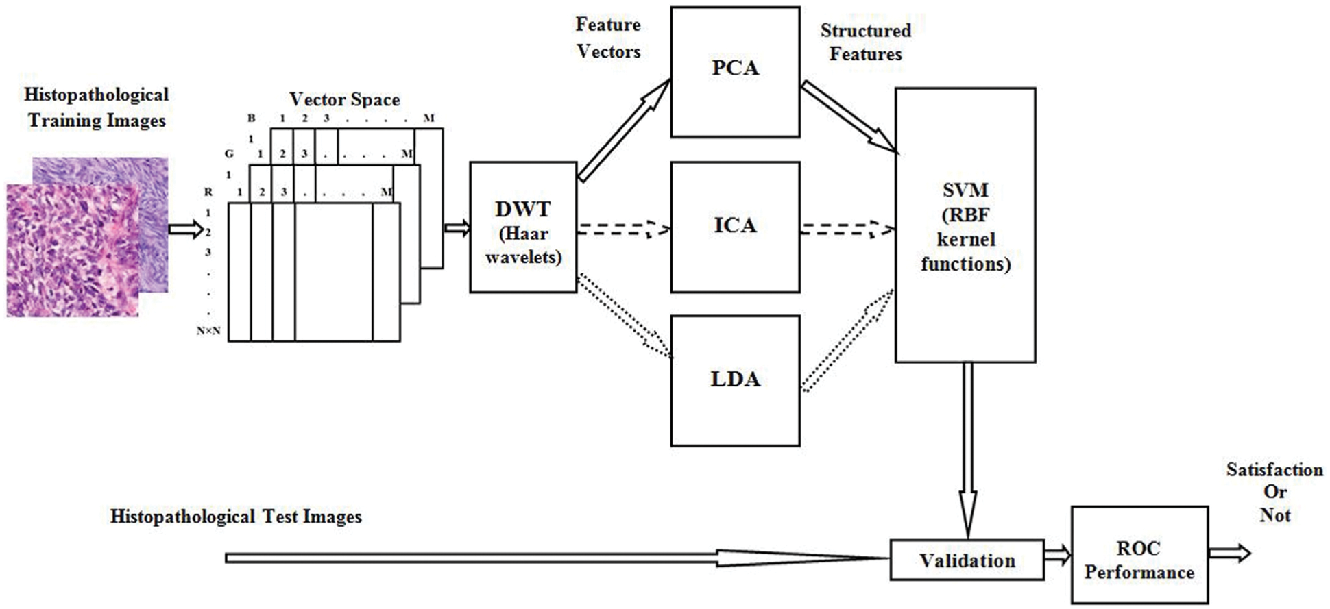
Figure 2: Block diagram of overall procedure and its internal operation of SSC structure classification

2.2 Fundamental of Wavelet Transform (WT)

An image is said to be stationary, then it does not change much over time. The Fourier transforms (FT) can be applied to the stationary images. But, the images have plenty of image pixel density value which contains stationary characteristics. Thus, it is not ideal to directly use the FT for such images; in such a situation sub-band techniques such as WT must be used. Wavelet analysis has been used for a variety of different probing functions [36]. This idea leads to state the equation for continuous wavelet transform (CWT) and defined as

W(u,v)=∫−∞∞⁡x(t)1uΨ∗(t−vu)dt(1)

where, the variable u acts as to vary the time scale of the probing function of Ψ, and v acts as to translate the function across x(t). If u<1 (but still positive) it contacts the function and if it u>1, the wavelet function Ψ is stretched along the time axis. While the probing function Ψ could be any of a number of different functions, it at all times take on an oscillatory waveform, is called the wavelet. The Ψ∗ indicates the complex conjugation of Ψ, and the normalizing factor of 1u ensures that the energy is the same for all values of the time scale u. In furthermore, the Haar transformations would be preferred a transform that produces the minimum number of coefficients required to recover accurately in the original signal/image. The standard Haar wavelet ψ(t) is defined by

Ψ(t)={+1for0≤t<0.5−1for0.5≤t<10Otherwise        (2)

DWT controls this parsimony translation and scale, functions, variation to powers of 2 in general. Filter banks are best described as the basis for most medical image processing applications, such as DWT-based analysis. The advantages of a group of filters to separate an image into different spectral components is called sub-band image. This approach is called as multi-resolution decomposition of the x[n] image. Each phase of the system consists of two digital filters and two down-samplers by 2. In nature, the first one is the high pass filter, h[.] is the distinctive mother wavelet and the other mirror version is the low pass filter g[.]. The down sampled releases the first high-pass and the low-pass filters provide detail and the approximation, respectively [37].

Appropriate wavelet and decomposition levels are most significant in the analysis of images using DWT. The number of decomposition levels is selected based on the dominant frequency components of an image. 2D-DWT acting as a 1D wavelet, it alternates rows and 1D-DWT columns. 2D-DWT works directly by placing an array transposition between two 1D-DWTs. Rows of arrays are initially managed only with one level of decomposition. It is basically divided into two equally vertical. The first half stores the average coefficients and the second vertical half save the detail coefficients. These steps are repeated with the column, resulting in four sub-band images within the array defined by the filter output as shown in Fig. 3, and these images are three-level 2D-DWT decomposition of the image. Each pixel value represents digital equivalent image intensity, with pixels set in the image 2D matrix. This is unnecessary because the adjacent pixel values are highly correlated in the spatial domain here. So to compress the images, these redundancies in pixels should be removed. It converts DWT spatial domain pixels into frequency domain information, so they are represented by multiple sub-bands images [38].

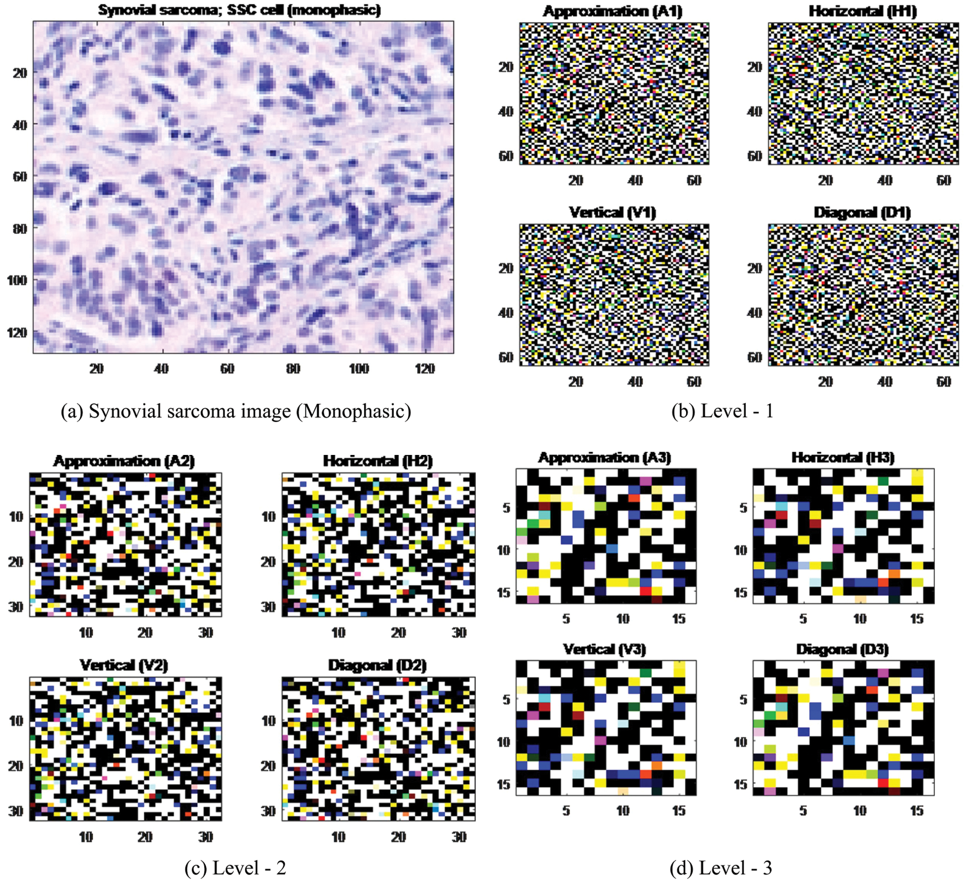
Figure 3: Levels of Haar wavelets sub-band images

In order to further reduce the dimensionality of the extracted structure feature vectors, the wavelet coefficient statistics value has been used to represent sub-band image distribution [39]. The statistical features are listed here: (1) Mean values of coefficients in each sub-band, (2) Standard deviation of coefficients in each sub-band, (3) Ratio of absolute mean values of the adjacent sub-band.

2.3 Structure Features Extraction Methods

Hematoxylin and eosin stain (H&E stain) is one of the chief tissue stains utilized in histology. It is the most broadly utilized stain in clinical conclusion and is regularly the best quality level. For instance, when a pathologist takes a gander at a biopsy of a presumed malignancy, the histological segment is probably going to be stained with H&E. It is the blend of two histological stains: hematoxylin and eosin. The hematoxylin stains cell cores a purplish blue, and eosin stains the extracellular lattice and cytoplasm pink, with different constructions, taking on various shades, tones, and mixes of these shadings. Thus a pathologist can undoubtedly separate between the atomic and cytoplasmic pieces of a cell, and furthermore, the general examples of shading from the stain show the overall format and dispersion of cells and gives an overall outline of a tissue test's construction. Accordingly, design acknowledgment, both by master people themselves and by programming that guides those specialists (in computerized pathology), gives histologic data.

The structure features (SFs) has been used to feature dimensionality for better optimized criterion related to dimensionality reduction techniques for other criteria. Lot of feature selection methods have been available to reduce dimensionality, extracting features, and removing noises before the cancer classification. First one is an input space feature selection, which reduces the dimensionality of the image by selecting a subset of features to conduct a hypothesis testing in a same space as the input image. Second one is the subspace feature selection or transform based selection, which reduces the image dimensionality by transforming images into a low dimensional subspace induced by linear or nonlinear transformation. The linear dimensionality reductions are commonly used method for image dimensionality reduction techniques in cancer classification. The popular linear dimensionality reduction techniques are, (1) Principal Component Analysis (PCA), (2) Independent Component Analysis (ICA), and (3) Linear Discrimination Analysis (LDA). The subspace feature selection methods have been mainly focused on this study.

2.3.1 Principal Component Analysis (PCA)

Principal Component Analysis, or PCA, is a dimensionality-decrease strategy that is frequently used to diminish the dimensionality of huge datasets, by changing a huge arrangement of factors into a more modest one that actually contains the majority of the data in the bigger set. PCA can be depicted as an “unsupervised” algorithm, since it “disregards” class names and its objective is to discover the bearings (the supposed head segments) that amplify the change in a dataset. Decreasing the quantity of factors in a dataset normally comes to the detriment of exactness, yet the stunt in dimensionality decrease is to exchange a little precision for straightforwardness. Since more modest informational collections are simpler to investigate and picture and make examining information a lot simpler and quicker for AI calculations without superfluous factors to measure.

In PCA, the mathematical representation of linear transformations of original image vector into projection feature vector [40] is given by

Y=WTX(3)

where, Y is the m×N feature vector matrix, m is the dimension of the feature vector, and transformation matrix W is an n×m, whose columns are the eigenvectors (λ) corresponding to the eigenvalues (I) computed using λI=SI. Here, the total scatter matrix S is defined as the average image of all samples.

S=∑i=1N⁡(xi−μ)(xi−μ)T(4)

where, μ=1N∑i=1N⁡xi. After using the linear transformation WT, the scatter of the transformed feature vectors {y1,y2,…,yn} is WTSW. In PCA, the projection W is selected to increase the resolution of the S of the projected samples, that is

W=argMAXw|WTSW|=[w1,w2,…,wm](5)

where, w1,w2,…,wm is the set of n-dimensional eigenvectors of S, and m is corresponding largest eigenvalues of S. In other words, the input vector in n-dimensional space is reduced to a feature vector in m-dimensional subspace. As a result, the dimension of the reduced feature vector m is much less than the dimension of input image vector n.

2.3.2 Independent Components Analysis (ICA)

The Independent Components Analysis (ICA) is statistical parameter feature extraction methods that transform a multivariate random signal into a signal having components that are mutually independent and it can be extracted from the mixed signal. The ICA rigorously defines as the statistical “latent variable” model [41,42]. Let n linear mixtures x1,x2,…,xn of n independent components.

xj=aj1s1+aj2s2+⋯+ajnsn,∀j(6)

ICA models have now dropped time index t, where xj is the each mixture. In addition, each independent component sk is a random variable that converts a real-time signal image. Here, the observed values xj(t), the mixture variables and the independent components are assumed to be zero mean. If it is not true, then observable variable xi has consistently been centred by subtracting the sample mean, and which is made the model zero mean. For our convenient to use vector matrix notation as an alternative of sums like in the Eq. (6). Let x be the random vectors with elements is the mixtures x1,x2,…,xn and similarly s be the random vector whose elements has been the mixtures s1,s2,…,sn. Let A be a matrix, whose components are aij. All vectors are understood to be column vectors; this vector xT is a row vector. Eq. (7) is rewritten using this vector matrix notation.

x=As(7)

Suppose, the required columns of matrix A and indicated by aj, then the model equation can thus be changed as

x=∑i=1n⁡aisi(8)

Eq. (8) is called the ICA model or generative model which describes how the observed data are generated by the process of mixing the components of si. The latent variables are independent component, which they can be indirectly observed. Also, let us consider the mixing matrix is to be unknown. The random vector x is observing all and must evaluate the both A and s using it.

The ICA starting point is very simple considering that component si are statistically independents and it must also have non-Gaussian distributions. The determination of matrix A and the calculation of its inverse matrix W are used to obtain the independent component.

s=Wx(9)

Let W=A−1, but neither A nor its inverse are known and the determination of A by maximum-likelihood techniques.

2.3.3 Linear Discriminant Analysis (LDA)

Linear Discriminant Analysis or Normal Discriminant Analysis or Discriminant Function Analysis is a dimensionality decrease procedure which is ordinarily utilized for the managed characterization issues. It is utilized for displaying contrasts in gatherings, for example, isolating at least two classes. It is utilized to extend the highlights in higher dimensional space into a lower measurement space. For instance, we have two classes and we need to isolate them productively. Classes can have different highlights. Utilizing just a solitary component to order them may bring about some covering. Along these lines, we will continue expanding the quantity of highlights for legitimate arrangement. PCA can be portrayed as an “unsupervised” algorithm, since it “disregards” class marks and its objective is to discover the bearings (the alleged head segments) that augment the difference in a dataset. LDA is “managed” and processes the bearings (“linear discriminants”) that will address the tomahawks that expand the partition between different classes.

The main goal of the LDA is to discriminate the classes by projecting class samples from p-dimensional space onto a finely orientated line. For a N-class problem, m=min(N−1;d) different orientated line will be involved in [43]. For example, the analysis has N-classes, X1,X2,…,XN. Let the ith observation vector from the Xj be xji, where j=1,2,…,J and i=1,2,…,Kj. J is the number of classes and Kj is the number of observations from class j. The co-variance matrix is determined in two ways (1) within-class co-variance matrix CW, and (2) between-class co-variance matrix CB.

Cw=∑j=1N⁡Cj=∑j=1N⁡1Kj∑i=1Kj⁡(xji−μj)(xji−μj)T(10)

CB=∑j=1N⁡Nj(μj−μ)(μj−μ)T(11)

where, μj=1Kj∑i=1Kj⁡xji and μ=1K∑i=0K⁡xi are mean of class j and global mean, respectively.

The projection of observable space into feature is accomplished through a linear transformation matrix T:

y=TTx(12)

The corresponding within-class covariance matrix C¯W and between-class covariance matrix C¯B in the feature space are given as

C¯W=∑j=1N⁡∑i=0Kj⁡(yji−μ¯j)(yji−μ¯j)T(13)

C¯B=∑j=1N⁡Kj(μ¯j−μ¯)(μ¯j−μ¯)T(14)

where, μ¯j=1Kj∑i=1Kj⁡yji and μ¯=1K∑i=0K⁡y¯i, it is honest to show that:

C¯W=TTSWT(15)

C¯B=TTSBT(16)

The linear discriminant is then defined as a linear function for which the objective function J(T) is given as

J(T)=|C¯B||C¯W|=|TTCBT||TTCWT|(17)

Here, the value of J(T) is the maximum and the solution of the Eq. (17) is the optimal transformation matrix T of the ith column, which is the common eigenvector corresponding to the ith largest eigenvalue of the matrix of CW−1WSB. To obtain the discriminant profile, the LDA classification score (Lik) for a given class k is calculated by the Eq. (18) and it is considered equivalent to the class covariance matrices:

Lik=(Xi−X¯k)T∑pooled−1⁡(Xi−X¯k)−2logeπk(18)

where, Xi is a measurement vector unknown to a sample   I; Xk is the mean measurement vector of class   k; Σpooled is a pooled covariance matrix; and πk is the prior probability of class k [42].

2.4 The Constructing of Support Vector Machine (SVM)

Let us consider the case of two classes α1 and α2, and the training dataset is X={x1,x2,…,xN}⊂PR. The Eq. (19) is formed as rules by the training data [44].

yi={+1,xi∈α1−1,xi∈α2(19)

In appearance, SVM is binary classifier and it can evolution of image data points and assign them to one of the two classes. The input observation vectors are projected into higher dimensional feature space F. The function f(x) takes the form

f(x)=(v⋅θ(x))+b(20)

With θ:PR→F and v ∈ F, where (⋅) is denoted by the dot product. Often, all desirable data in these two classes meet the constraints in Eq. (21)

yj(v⋅θ(xi))+b−1≥0,∀i(21)

Eq. (21) can be described as a hyperplane, where, v and b are described as the position of the corresponding region to coordinate the vector and centre of the hyperplane, respectively.

The optimization of this margin to its SVs can be converted into a constrained quadratic programming problem as seen in Eq. (21). This problem can be rewritten as optimization statements.

Minimize12||v||2+C∑i=1N⁡ξi(22)

Subject toyi(vT⋅θ(xi))+b≥1−ξi,∀i(23)

where, Eq. (22) is the primary objective function and Eq. (23) is the relative constraint of the objective function. Where, ξi is the slack variable, which indicates the misclassified of the corresponding margin hyperplane, and C is the parameter indicates the cost of the penalty. It is used to reduce the error if it is too large or to increase the size of the margin if it is too small.

The Eqs. (22) and (23) can be solved by creating a Lagrange function. Hence, the positive Lagrange multipliers are taken consideration ωi;i=1,2,…,N, one for each constraint in both Eqs. (22) and (23). The Lagrange function [45] is defined by

Lp=12||v||2−∑i=0N⁡ωi(yi(v⋅θ(xi))+b)+∑i=1N⁡ωi(24)

The gradient of Lp must be minimized with respect to both v and b value, and they must vanish. The gradients are given by

∂LP∂vs=vs−∑i=1N⁡ωiyiθ(xis)=0,s=1,2,…,p(25)

∂LP∂b=−∑i=1N⁡ωiyi=0(26)

where p is the dimension of feature space F, and by combining these conditions, the primary function, constraints of the Lagrange multipliers, and the Karush-Kuhn-Tucker (KKT) conditions are obtained. They are defined as in Eqs. (27)–(31).

∂LP∂vs=vs−∑i=1N⁡ωiyiθ(xis)=0,s=1,2,…,p(27)

∂LP∂b=−∑i=0n⁡ωiyi=0(28)

yi(v⋅θ(xi))+b−1≥0∀i(29)

ωi≥0∀i(30)

ωi(yi(v⋅θ(xi))+b−1)=0∀i(31)

Here, the v,b and ω are variables to be solved from the KKT Eq. (26) and derived as

v=∑i=1N⁡ωiyiθ(xi)(32)

∑i=1N⁡ωiyi=0(33)

Therefore,

f(x)=∑i=0N⁡ωiyi(θ(xi)⋅θ(x))+b(34)

=∑i=0N⁡ωiyil(xi,x)+b(35)

where l(xi,x)=(θ(xi)⋅θ(xj)) is the kernel function that uses the dot product at F in the feature-space; Also, substitute Eqs. (24)–(33), which leads to increase the dual function LD.

LD=−12∑i=0N⁡∑j=1N⁡ωiωjyiyjlij+∑i=0N⁡ωi(36)

Here, define the dual function which incorporates the constraints, and obtain the dual optimization problem.

Maximize    −12∑i=1N⁡∑j=1N⁡ωiωjyiyjlij+∑i=1N⁡ωi(37)

Subject to  ∑i=1N⁡ωiyi=0(38)

ωi≥0∀i(39)

Both primal Lp and the dual LD constraints are represented by the same objective function, but with different constructions. This optimization of the primal dual constraints is considered as a type of convex optimization problem and it can be rectified by using the grid-search algorithm. Finally, the SVM classifier classifies the input data vector x by the classification criteria in Eq. (40).

x∈Classi,    if  f(i)(x)=max∀j∈M⁡f(j)(x)(40)

where, M-dimensional value vector f(i)(x), i=1,2,…,M is generated.

In this study, the SVM algorithm is analyzed using the RBF kernel, which can be easily formatted for any other kernel function. It also has tuning parameter to optimize performance [46–48] and defined as

l(xi,x)=exp⁡(−γ‖xi−xj2‖)+β(41)

where, l(xi,x) is the positive definite for a value in RBF kernel case, γ=12σ2 is the tuning parameter which controls the width of the kernel function, and σ is the standard division.

Support Vector Machine (SVM) is a supervised machine learning algorithm which can be used for both classification and regression challenges. It aims to minimize the number of misclassification and reconstruction errors. It is used in all the real-world applications, where the data are linearly inseparable. The SVMs implemented in this research were used as classifiers for the final stage in a multistage automatic target recognition phase. A single kernel SVM in this research may be used as an SVM with K-Means Clustering. Here, Support Vectors (SVs) are simply the co-ordinates of individual observation. We plot each data item as a point in n-dimensional space (where n is a number of features) with the value of each feature being the value of a particular coordinate. Then, we perform classification by finding the hyperplane that differentiates the two classes very well.

At this stage, the reconstruction error may be occurring in the distance between the original data point and its projection onto a lower-dimensional subspace. This reconstruction error is a function of the outputs and the weights. It may be calculated from a given vector, which is to compute the Euclidean distance between it and its representatives. In K-means, each vector is represented by its nearest center. Minimizing the reconstruction error means minimizing the contribution of ignoring eigenvalues which depend on the distribution of the data and how many components we are selecting. So the SVM based learning is to adapt the parameters which can minimize the average reconstruction error made by the network.

3  Experiment Results

A few examples are utilized as usefully focuses to oversee enormous component spaces through the SVM classifier to abstain from over-fitting cell structures by controlling the edge, and they are called support vectors (SVs). Through these SVs the proposed calculation can tackle the current issues. The arrangement won't generally change if these preparation datasets are re-prepared. The preparation can guarantee that SVs can address every one of the attributes in the dataset. This is viewed as a significant property while investigating huge datasets with numerous uninformative designs. All in all, the quantity of SVs is more modest than the complete preparing dataset. In any case, this doesn't change overall preparation information into SVs. In this experiment, the 64 SVs are utilized for dynamic interaction (Figs. 4–6), showed a circle; the green circle ‘○’ is utilized for SVs in the SSC structure class and the red circle ‘○’ portrays SVs for non-SSC structure class. The class areas are isolated by a hyperplane.

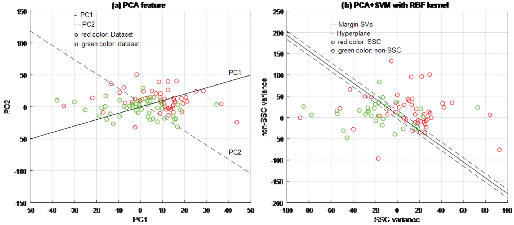
Figure 4: PCA + SVM classifier model

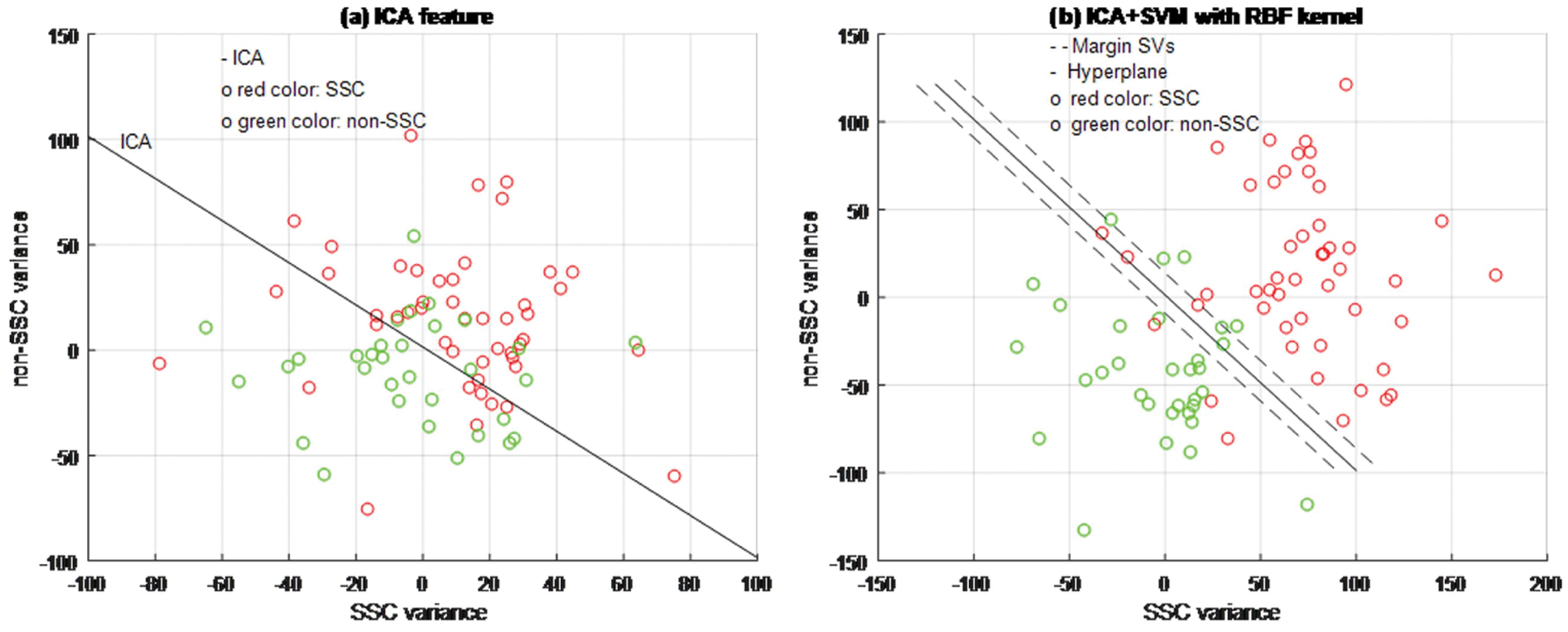
Figure 5: ICA + SVM classifier model

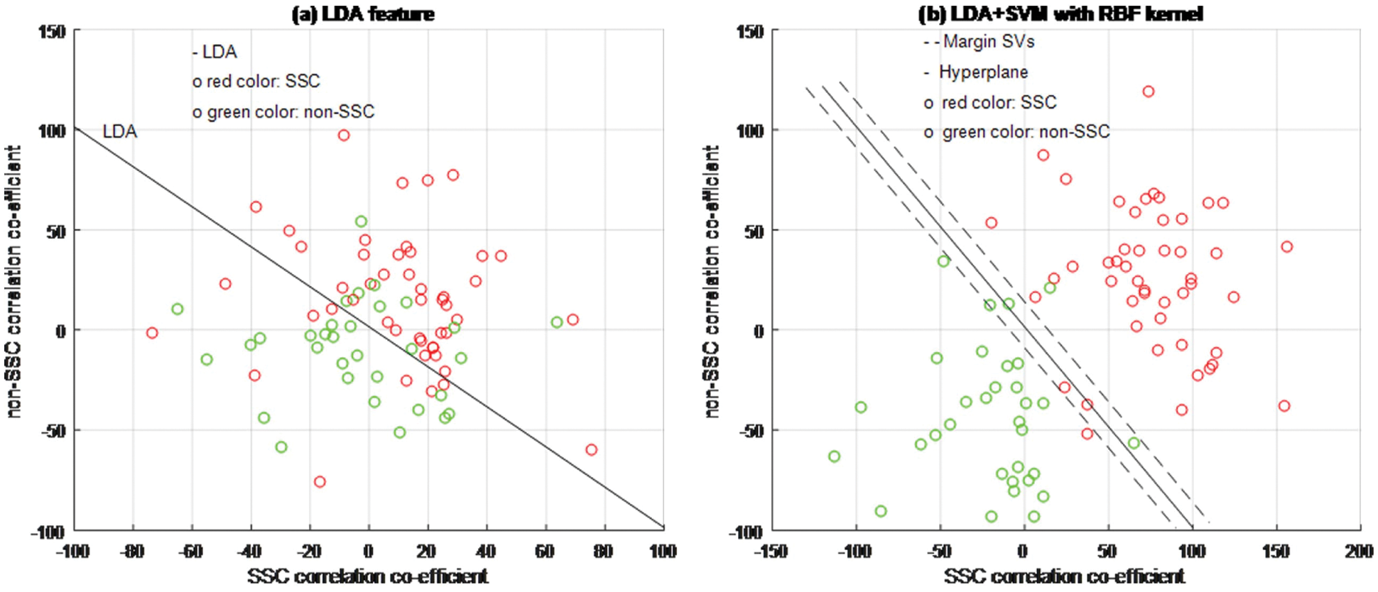
Figure 6: LDA + SVM classifier model

Based on experimental results, Figs. 4a, 5a and 6b are shown the two-dimensional (2D) scatter plots of cell structures from the third level of the Haar wavelets (feature vectors). The acquisition of the third-level of the sub-band image detail approximation (A3) structured features have been extracted for the structure of the SSC (‘○’-red color circle) and non-SSC (‘○’-green color circle) of the two classes. Visually, it is difficult to separate data dispersion into two classes, so using a linear separable hyperplane can cause overlapping problems. This has an impact on errors in the classification process. In such case, a kernel function is required to convert the data into high dimensional space. Based on this, the cell structures of the two groups of histopathological image can be easily separated.

In this work, the RBF kernel SVM classifier with two corresponding tuning parameters such as β and γ plays a key role in model performance. As a result, both of these parameters result an excessive fit for inappropriate selection. Therefore, the proposed methodology found the optimal tuning parameter values, which led to the classifier to accurately classify the data input. Furthermore, this methodology used 5-fold for cross-validation to implement the appropriate kernel tuning parameters for β and γ. Most importantly, all pairs (β, γ) for the RBF kernel are accessible, and the best of them is cross-validation accuracy. The optimal tuning parameter pair values were β=2−1, γ=2−3 and the classification error rate was 0.15. After selecting the value of the optimal kernel tuning parameters, the entire training data is re-trained in the construction of the final classifier.

The structure of the cell is classified and the performance results have been compared with SEs methods such as PCA, ICA, and LDA by SVM classifier with RBF kernel functions which shown in Figs. 4b, 5b and 6b. The dimensionality of the cell structures has been reduced by using the structural features. SVM with kernel classification model has been implanted using these structural feature datasets as inputs. In the classifier result, if the SSC structure is provided with output, it represents SS cancer, and if non-SSC structure is provided with output, it represents non-cancerous.

The training process examines the RBF kernel in three different ways: (1) PCA + SVM, (2) ICA + SVM, and (3) LDA + SVM. Using PCA, ICA, and LDA types of SFs methods, the cell structures’ feature vectors are extracted from Haar wavelet sub-band image (A3) individually. The number of SVs is decreased and the classification test results have been analyzed by internal and external cross-validations. Fig. 6b explains the separation of cell structures when the distribution along with the LDA + SVM model indicates the mass of correlation co-efficient values of the two classes of data points which has been exactly distributed, towards the up-right and down-left side portions. But, one or two data points are occupied in the nearby SVs margin. Fig. 5b explains the separation of cell structures when the distribution along with the ICA + SVM model indicates the mass of variance matrix value of two classes of data points. Then the maximum number of data points has been distributed, towards the up-right and down-left side portions. But, few numbers of data points are occupied in the nearby hyperplane. Fig. 4b explains the characteristics of data classification separated based on its highest PC1 variance value. The separation of cell structures when the distribution along with the PCA + SVM model indicates the mass of PC1 variance value of the two classes of data points. Then the moderate number of data points has been distributed towards the up-right side and down-left side portions. When compared to ICA + SVM, more number of data points is occupied on the nearby hyperplane in both cell structures. Furthermore, the mass of data has been separated into two classes using SVM hyperplane and each of the groups. Here, the best boundary discrimination has been achieved by the RBF kernel function. The LDA + SVM have been achieved excellent performance of classification method and it has shown by the number of SVs, which has reduced than the ICA + SVM and PCA + SVM.

In this context, a classification using LDA feature extraction required less number of SVs than PCA feature exaction method. Moreover, the feature extraction classification process requires a lower number of SVs for the ICA than the PCA. The ICA measurements are described not only as unrelated to cell structural components but also as independent. Therefore, it is used for classification in terms of more valuable independent components than its related components.

However, the LDA + SVM feature extraction process takes longer duration in the training process than the ICA + SVM and the PCA + SVM feature extraction methods. Moreover, it has a transparent selecting scheme for the kernel function tuning parameters which are a pivotal to get better performance characteristics and overcome the problems of over-fitting with excellent classification process.

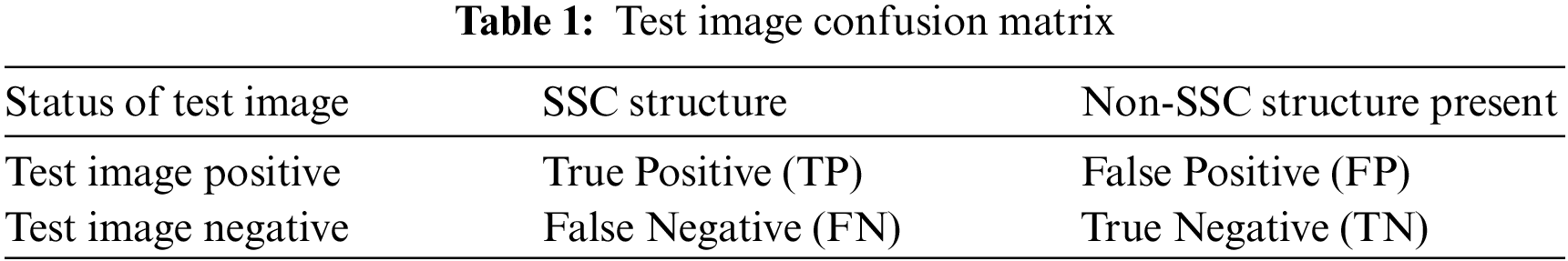
Before making any predictions about whether or not the histopathological images are affected by SSC structure, it is necessary to train the data by the characteristics associated with the test samples of the known class. Next, with the same datasets, the performance of the classification models is evaluated. The proposed work evaluated the classification performance by using the ROC curve. The relative tradeoffs between the sensitivity of the y coordinates and 1-specificcity as the x coordinate are shown in ROC curve. Fig. 7 shows the ROC curve and useful for assigning the best cutoffs to the classification [49]. These two parameters are mathematically expressed as sensitivity = TP/(FN + TP) and specificity = TN/(FP + TN). Tab. 1 shows the test images with confusion matrix. The threshold for the best cutoff ranges between 0-to-1 is considered uniformly with 0.02 intervals, and it gives totally 50 samples per parameters.

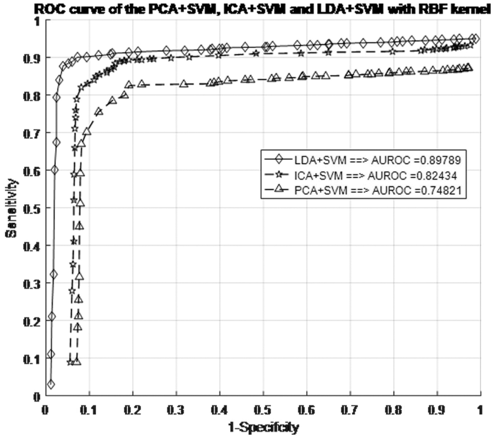
Figure 7: ROC curve for different SFs in the SVM + RBF classifiers with RBF kernel models

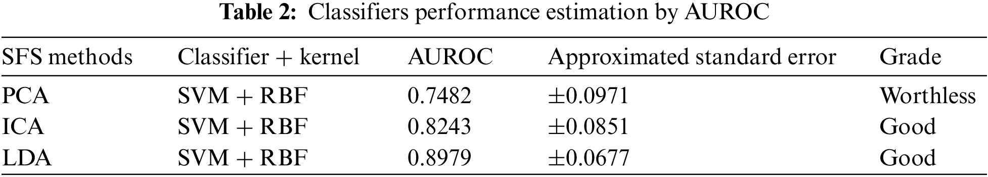
The most common quantity index for describing accuracy is given by the area under the ROC curve (AUROC). AUROC is used as an analytical tool for evaluating and comparing classifiers, and also provides measurable quantities such as accuracy and approximate standard error rate [50]. This curve is used to classify and regulate the performance regardless of class distribution. ROC curve measurement is classified into negative and positive classes in the result code for desirable properties and performance. Furthermore, AUROC can also be determined by the Eq. (42). Tab. 1 summarizes the AUROC performance results and approximated standard error of the PCA + SVM, ICA + SVM and LDA + SVM classification models with different kernel functions.

AUROC  =  ∑iN−1⁡((1−specificity)i+1−(1−specificityi)∗(sensitivityi+sensitivityi+1))/2(42)

The AUROC grade system is generally categorized into four groups, which are excellent, good, worthless and not good. Their common range values are 0.9<AUROC<1.0, 0.8<AUROC<0.9, 0.7<AUROC<0.8 and 0.6<AUROC<0.7, respectively. Hence, Fig. 7 shows the result of AUROC values for PCA + SVM, ICA + SVM and LDA + SVM with RBF kernel function, and they have the AUROC of 0.7482, 0.8243, and 0.8979, respectively. Depending on these AUROC values, not good, worthless and good are described as PCA + SVM, ICA + SVM and LDA + SVM classification models, respectively. Whereas the LDA + SVM with RBF is a good model, and it is demonstrated that has been chosen to be applied in the proposed SSC structure classification, because this classifier model has greatest AUROC than the others.

The LDA + SVM with RBF model is compatible with taxonomic sources as it has the lowest approximate standard error in the creation of a hyperplane model which shows in the Tab. 2. There is an attractive difference between two analyses. It means a ROC curve against the occurrence of the classification error and the other two classifiers. However, the ROC curve analysis is useful for performance evaluation in the current framework because it reflects the true state of classification problem rather than a measurement of classification error [51–53].

4  Discussion

The present study reaffirms the existence of training databases based on evaluation of the classification models by using different types of SFs and RBF kernel functions. Blockchain technology allows SVM models to be trained with a large number of decentralized high-quality SS image data from IoT networks. The structural features of SVs are stored on IoT devices and periodically trained for SVM classification. The LDA structure feature and the SVM with RBF kernel were selected as a classification model. If the red circle resultant from the f(x) calculation value in the rule Eq. (35) of the RBF kernel is denoted by (‘◯’), and it is classified as a SSC structure. Conversely, the diagnosis of SS cancer may assist pathologists in the progression and prognosis of chronic disease from the histopathological image.

SVM is based on cell structures with high dimensional spacing, which is usually much larger than the original structured feature space. The two classes are always separated by a hyperplane with a non-linear map suitable for an acceptable high dimensional dataset. While the original structured feature brings enough information for better classification, the mapping of the high-dimensional structured feature space makes available in the best discriminating sources. Hence, the problem with training for SVM is that the nonlinear input is mapped to a higher dimensional space and selection of the classification function. The RBF kernel function is used for the training of SVM. The values of optimal RBF tuning parameters β and γ have been identified through grid-search technique. An SVM classifier with RBF kernel provides better experimental results based on the integrated training [54–56]. However, other common optimal parameter searching methods are available such as deep learning algorithms, particle swarm optimization, and genetic algorithm [57]. So, this is an interesting topic to explore further.

Tab. 3 shows the overall performance comparison between SFs methods and RBF functions. The Gini index is a primary parameter that measures the superior performance between the classifiers. It is based on the area dominated by the ROC surfaces. The determination of Gini coefficient from the ROC curve is given by

G=1−∑k=1n⁡((1−specificity)k−(1−specificity)k−1)∗(sensitivityk+sensitivityk−1)(43)

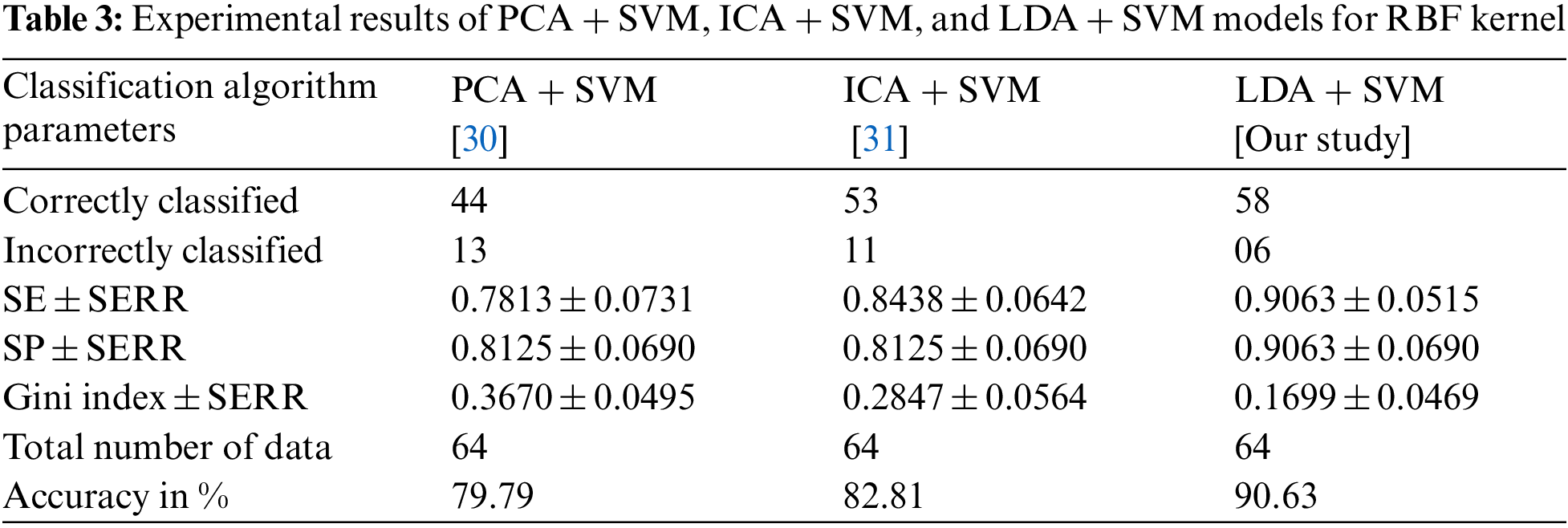
The proposed classification model has shown the robustness of classifying SS cancer effectively and accurately in LDA + SVM with RBF kernel function. The standard error (SERR) is specified in each parameter to understand the maximum and minimum variations in sensitivity (SE), specificity (SP) and Gini index. The LDA + SVM have obtained a higher classification rate than the other classifier models.

The success rate of the proposed classification methodology depends on the structural features and its selection process of a cell. The classification performance is improved by the transformation patterns of the SFs which reduces the with-class scatter, increases the between-class scatter, and significantly reduces the size of overlap between the classes. Statistically, PCA, ICA and LDA structural features are distinguished between normal image and SS cancer image due to the easy computation, simplicity, and rapid implementation.

5  Conclusion

Classification of cancer based on the malignant cell structure in histopathology images is a very difficult task. Hence, SVM classifiers used to classify the cell structure and assists to pathologists for diagnostic decision making. The conventional classification techniques of histopathology images using mutually exclusive time and frequency domain representations are not provided the proficient results. In this work, the histopathology images have been decomposed into sub-band using Haar DWT and then the SFs are extracted by obsessed their distribution. The extraction of SFs may be possible in three different ways: PCA, ICA, and LDA. These methods are used SVMs with RBF kernel functionality. The extraction results are compared with the observed cell structures and then cross-compared with their accuracy. The scalar performance measures like accuracy, specificity and sensitivity are derived from the confusion matrices. Results of the histopathological image classification by using SVMs are shown the nonlinear SFs datasets can provide the better performance characteristics of the classifier when reducing the number of SVs. Hence, the use of nonlinear SFs datasets and SVM with RBF kernel function may be served as a diagnostic tool in modern medicine. Besides, the interpretive performance of SVM can be improved by dimensionality reduction of PCA, ICA, and LDA. Likewise, blockchain technology may be used in the deep learning technique as a storage system and sharing of SS image data over a secure IoT network. This secured electronic health imaging data may be stored in the planetary file system with the latest support vector's values. Therefore, recent support vectors and different structural features may be available for future works to achieve integrated blockchain technology based SS image data classification and pharmaceutical industry applications.

Acknowledgement: Our heartfelt thanks to Dr. S. Y. Jegannathan, M.D (Pathologist), DPH, Deputy Director of Medical Education, Directorate of Medical Education, Kilpauk, Chennai, Tamil Nadu, India, who provided valuable advice and oversight in guiding our work.

Funding Statement: This work was partly supported by the Technology development Program of MSS [No. S3033853] and by Basic Science Research Program through the National Research Foundation of Korea (NRF) funded by the Ministry of Education (No. 2020R1I1A3069700).

Conflicts of Interest: The authors declare that they have no conflicts of interest to report regarding the present study.

References

 1.  W. Wang, J. A. Ozolek, D. Slepcev, A. B. Lee, C. Chen et al., “An optimal transportation approach for nuclear structure based pathology,” IEEE Transactions on Medical Imaging, vol. 30, no. 3, pp. 621–631, 2015. [Google Scholar]

 2.  M. D. Murphey, M. S. Gibson, B. T. Jennings, A. M. Crespo-Rodriguez, J. Fanburg-Smith et al., “From the archives of the AFIR: Imaging of synovial sarcoma with radialogic-pathology correlation,” Radiographics: A Review Publication of the Radiology of the Society of North America, Inc., vol. 26, no. 5, pp. 1543–1565, 2006. [Google Scholar]

 3.  A. Kerouanton, I. Jimenez, C. Cellier, V. Laurence, S. Helfre et al., “Synovial sarcoma in children and adolescents,” Journal of Pediaatric Hematology/Oncology, vol. 36, no. 4, pp. 257–262, 2014. [Google Scholar]

 4.  K. Thway and C. Fisher, “Synovial sarcoma: Defining features and diagnostic evolution,” Annals of Diagnostic Pathology, vol. 18, no. 6, pp. 369–380, 2014. [Google Scholar]

 5.  G. Rea, F. Somma, T. Valente, G. Antinolfi, G. D. Grezia et al., “Primary mediastinal giant synovial sarcoma: A rare case report,” The Egyptian Journal of Radiology and Nuclear Medicine, vol. 46, no. 1, pp. 9–12, 2015. [Google Scholar]

 6.  R. Ershadi, M. Rahim and H. Davari, “Primary mediastinal synovial sarcoma: A rare case report,” International Journal of Surgery Case Reports, vol. 27, pp. 169–171, 2016. [Google Scholar]

 7.  K. J. Khouzani and H. S. Zadeh, “Mutiwavelet grading of pathological images of prostate,” IEEE Transactions on Biomedical Engineering, vol. 50, no. 6, pp. 697–704, 2003. [Google Scholar]

 8.  N. Aydin, S. Padayachee and H. S. Markus, “The use of the wavelet transform to described embolic signals,” Ultrasound in Medicine and Biology, vol. 25, no. 6, pp. 953–958, 1999. [Google Scholar]

 9.  S. G. Mallat, “A theory for multiresolution signal decomposition: The wavelet representation,” IEEE Transactions on Pattern Analysis and Machine Intelligence, vol. 11, no. 7, pp. 674–693, 1989. [Google Scholar]

10. B. Lessmann, T. W. Nattkemper, V. H. Hans and A. Degenhard, “A method for linking computed image features to histological semantics in neuropathology,” Journal of Biomedical Informatics, vol. 40, no. 6, pp. 631–641, 2007. [Google Scholar]

11. A. Tabesh, M. Teverovskiy, H. Y. Pang, V. P. Kumar, D. Verbel et al., “Multifeature prostate cancer diagnosis and gleason grading of histopathological images,” IEEE Transactions on Medical Imaging, vol. 26, no. 10, pp. 1366–1378, 2007. [Google Scholar]

12. A. C. Roa, J. C. Caicedo and F. A. Gonzalez, “Visual pattern mining in histology image collections using bag of features,” Artificial Intelligence in Medicine, vol. 52, no. 2, pp. 91–106, 2011. [Google Scholar]

13. X. Castillo, D. Yorkgitis and K. Preston, “A study of multidimensional multicolor images,” IEEE Transactions on Biomedical Engineering, vol. 29, no. 2, pp. 111–121, 1982. [Google Scholar]

14. M. Ganga, N. Janakiraman, A. K. Sivaraman, A. Balasundaram, R. Vincent et al., “Survey of texture based image processing and analysis with differential fractional calculus methods,” in Int. Conf. on System, Computation, Automation and Networking (ICSCANIEEE Xplore, Puducherry, India, pp. 1–6, 2021. [Google Scholar]

15. J. P. Thiran and B. Macq, “Morphological feature extraction for the classification of digital images of cancerous tissues,” IEEE Transactions on Biomedical Engineering, vol. 43, no. 10, pp. 1011–1020, 1996. [Google Scholar]

16. Y. Smith, G. Zajicek, M. Werman, G. Pizov and Y. Sherman, “Similarity measurement method for the classification of architecturally differentiated images,” Computers and Biomedical Research, vol. 32, no. 1, pp. 1–12, 1999. [Google Scholar]

17. P. W. Huang and Y. H. Lai, “Effective segmentation and classification for HCC biopsy images,” Pattern Recognition, vol. 43, no. 4, pp. 1550–1563, 2010. [Google Scholar]

18. S. Doyal, M. Feldman, J. Tomaszewski and A. Madabhushi, “A boosted Bayesian multiresolution classifier for prostate cancer detection from digitized needle biopsies,” IEEE Transactions on Biomedical Engineering, vol. 59, no. 5, pp. 1205–1218, 2012. [Google Scholar]

19. O. S. Al-Kadi, “A multiresolution clinical decision support system based on fractal model design for classification of histological brain tumours,” Computerized Medical Imaging and Graphics, vol. 41, pp. 67–79, 2015. [Google Scholar]

20. Y. Ding, M. C. Pardon, A. Agostini, H. Faas, J. Duan et al., “Novel methods for microglia segmentation, feature extraction, and classification,” IEEE/ACM Transactions on Computational Biology and Bioinformatics, vol. 14, no. 6, pp. 1366–1377, 2016. [Google Scholar]

21. F. A. Spanhol, L. S. Oliveira, C. Petitjean and L. Heutte, “A dataset for breast cancer histopathological image classification,” IEEE Transactions of Biomedical Engineering, vol. 63, no. 7, pp. 1455–1462, 2016. [Google Scholar]

22. Y. Xu, Z. Jia, L. Wang, Y. Ai, F. Zhang et al., “Large scale tissue histopathology image classification, segmentation, and visualization via deep convolutional activation features,” BMC Bioinformatics, vol. 18, no. 281, pp. 1–17, 2017. [Google Scholar]

23. J. Kong, O. Sertel, H. Shimada, K. L., Boyer, J. H. Saltz et al., “Computer–aided evaluation of neuroblastoma on wholeslide histology images: Classifying grade of neuroblastic differentiation,” Pattern Recognition, vol. 42, no. 6, pp. 1080–1092, 2009. [Google Scholar]

24. R. Kumar, W. Y. Wang, J. Kumar, T. Yang, A. Khan et al., “An integration of blockchain and AI for secure data sharing and detection of CT images for the hospitals,” Computerized Medical Imaging and Graphics, vol. 87, no. 6, pp. 1–41, 2021. [Google Scholar]

25. R. Priya, S. Jayanthi, A. K. Sivaraman, R. Dhanalakshmi, A. Muralidhar et al., “Proficient mining of informative gene from microarray gene expression dataset using machine intelligence,” Advances in Parallel Computing, vol. 38, pp. 417–422, 2021. [Google Scholar]

26. U. Bodkhe, S. Tanwar, K. Parekh, P. Khanpara, S. Tyagi et al., “Blockchain for industry 4.0: A comprehensive review,” IEEE Access, vol. 8, pp. 79764–79800, 2020. [Google Scholar]

27. J. Clark and F. Provost, “Unsupervised dimensionality reduction versus supervised regularized for classification from sparse data,” Data Mining and Knowledge Discovery, vol. 33, pp. 871–916, 2019. [Google Scholar]

28. H. Ahn, E. Choi and I. Han, “Extracting underlying meaningful features and cancelling noise using independent component analysis for direct marketing,” Expert Systems with Applications, vol. 33, no. 1, pp. 181–191, 2007. [Google Scholar]

29. J. Nalepa and M. Kawulok, “Selection training sets for support vector machines: A review,” Artificial Intelligence Review, vol. 52, no. 2, pp. 857–900, 2019. [Google Scholar]

30. B. Scholkopf, K. K. Sung, C. J. C. Burges, F. Girosi, P. Niyogi et al., “Comparing support vector machines with Gaussian kernels to radial basis function classifiers,” IEEE Transactions on Signal Processing, vol. 45, no. 11, pp. 2758–2765, 1997. [Google Scholar]

31. C. Cortes and V. Vapnik, “Support-vector networks,” Machine Learning, vol. 20, no. 3, pp. 273–297, 1995. [Google Scholar]

32. W. Wang, M. Zhang, D. Wang and Y. Jiang, “Kernel PCA feature extraction and the SVM classification algorithm for multiple-status, through-wall, human being detection,” EURASIP Journal on Wireless Communications and Networking, vol. 151, no. 12, pp. 1–7, 2017. [Google Scholar]

33. H. Saberkari, M. Shamsi, M. Joroughi, F. Golabi and M. H. Sedaaghi, “Cancer classification in microarray data using a hybrid selective independent components analysis and u-support vector machine algorithm,” Journal of Medical Signals and Sensors, vol. 4, no. 4, pp. 291–298, 2014. [Google Scholar]

34. M. N. Gurcan, L. E. Bouncheron, A. Can, A. Madabhushi, N. M. Rajpoot et al., “Histopathological image analysis: A review,” IEEE Reviews in Biomedical Engineering, vol. 2, no. 6, pp. 147–171, 2009. [Google Scholar]

35. Y. Zhang, B. Zhang, F. Coenen, J. Xiao and W. Lu, “One-class kernel subspace ensemble for medical image classification,” EURASIP Journal on Advances in Signal Processing, vol. 2014, no. 1, pp. 1–13, 2014. [Google Scholar]

36. S. Mallat, “Multifrequency channel decompositions of images and wavelet models,” IEEE Transactions on Acoustics, Speech, and Signal Processing, vol. 37, no. 12, pp. 2091–2110, 1989. [Google Scholar]

37. B. P. Marchant, “Time frequency analysis for biosystem engineering,” Biosystems Engineering, vol. 85, no. 3, pp. 261–281, 2003. [Google Scholar]

38. R. Vincent, P. Bhatia, M. Rajesh, A. K. Sivaraman and M. S. S. Al Bahri, “Indian currency recognition and verification using transfer learning,” International Journal of Mathematics and Computer Science, vol. 15, no. 4, pp. 1279–1284, 2020. [Google Scholar]

39. M. Vetterli and C. Herley, “Wavelets and filter banks: Theory and design,” IEEE Transaction on Signal Processing, vol. 40, no. 9, pp. 2207–2232, 1992. [Google Scholar]

40. N. Emanet, H. R. Oz, N. Bayram and D. Delen, “A comparative analysis of machine learning methods for classification type decision problems in healthcare,” Decision Analytics, vol. 1, no. 6, pp. 1–20, 2014. [Google Scholar]

41. H. Kong, M. Gurcan and K. B. Boussaid, “Partitioning histopathology images: An integrated framework for supervised color-texture segmentation and cell splitting,” IEEE Transactions on Medical Imaging, vol. 30, no. 9, pp. 1661–1677, 2011. [Google Scholar]

42. A. Hyvarinen, “Fast and robust fixed-point algorithms for independent component analysis,” IEEE Transactions on Neural Networks, vol. 10, no. 3, pp. 626–634, 1999. [Google Scholar]

43. A. Hyvarinen and E. Oja, “Independent component analysis: Algorithms and applications,” Neural Network: The Official Journal of the International Neural Network Society, vol. 13, no. 4, pp. 411–430, 2000. [Google Scholar]

44. W. Wu, Y. Mallet, B. Walczak, W. Penninckx, D. L. Massart et al., “Comparison of regularized discriminant analysis, linear discriminant analysis and quadratic discriminant analysis applied to NIR data,” Analytica Chimica Acta, vol. 329, no. 3, pp. 257–265, 1996. [Google Scholar]

45. A. K. Jain, R. P. W. Duin and J. Mao, “Statistical pattern recognition: A review,” IEEE Transactions on Pattern Analysis and Machine Intelligence, vol. 22, no. 1, pp. 4–37, 2000. [Google Scholar]

46. N. H. Sweilam, A. A. Tharwat and N. K. A. Moniem, “Support vector machine for diagnosis cancer disease: A comparative study,” Egyptian Informatics Journal, vol. 11, pp. 81–92, 2010. [Google Scholar]

47. D. Bardou, K. Zhang and S. M. Ahmad, “Classification of breast cancer based on histology images using convolutional neural networks,” IEEE Access, vol. 6, pp. 24680–24693, 2018. [Google Scholar]

48. M. N. Asiedu, A. Simhal, U. Chaudhary, J. L. Mueller, C. T. Lam et al., “Development of algorithms for automated detection of cervical pre-cancers with a low-cost, point-of-care, pocket colposcope,” IEEE Transactions on Biomedical Engineering, vol. 66, no. 8, pp. 2306–2318, 2009. [Google Scholar]

49. M. Ganga, N. Janakiraman, A. K. Sivaraman, R. Vincent, A. Muralidhar et al., “An effective denoising and enhancement strategy for medical image using RL-GL-caputo method,” Advances in Parallel Computing, vol. 38, pp. 402–408, 2021. [Google Scholar]

50. A. P. Bradley, “The use of the area under the ROC curve in the evaluation of machine learning algorithms,” Pattern Recognition, vol. 30, no. 7, pp. 1145–1159, 1997. [Google Scholar]

51. A. Balasundaram, G. Dilip, M. Manickam, A. K. Sivaraman, K. Gurunathan et al., “Abnormality identification in video surveillance system using DCT,” Intelligent Automation & Soft Computing, vol. 32, no. 2, pp. 693–704, 2021. [Google Scholar]

52. S. H. Park, J. M. Goo and C. H. Jo, “Receiver operating characteristics (ROC) curve: Practical review for radiologist,” Korean Journal of Radiology, vol. 5, no. 1, pp. 11–18, 2004. [Google Scholar]

53. T. Fawcett, “An introduction to ROC analysis,” Pattern Recognition Letters, vol. 27, no. 8, pp. 861–874, 2006. [Google Scholar]

54. R. Kumar and A. Indrayan, “Receiver operating characteristics (ROC) curve for medical researchers,” Indian Pediatrics, vol. 48, no. 4, pp. 277–287, 2011. [Google Scholar]

55. R. Gayathri, A. Magesh, A. Karmel, R. Vincent and A. K. Sivaraman, “Low cost automatic irrigation system with intelligent performance tracking,” Journal of Green Engineering, vol. 10, no. 12, pp. 13224–13233, 2020. [Google Scholar]

56. T. Eitrich and B. Lang, “Efficient optimization of support vector machine learning parameters for unbalanced datasets,” Journal of Computational and Applied Mathematics, vol. 196, pp. 425–436, 2006. [Google Scholar]

57. S. W. Lin, K. C. Ying, S. C. Chen and Z. J. Lee, “Particle swarm optimization for parameter determination and feature selection of support vector machines,” Expert Systems with Application, vol. 35, no. 4, pp. 1817–1824, 2008. [Google Scholar]

This work is licensed under a Creative Commons Attribution 4.0 International License, which permits unrestricted use, distribution, and reproduction in any medium, provided the original work is properly cited.