DOI:10.32604/cmc.2022.025739
| Computers, Materials & Continua DOI:10.32604/cmc.2022.025739 | |
| Article |
Robust Prediction of the Bandwidth of Metamaterial Antenna Using Deep Learning
1Department of Computer Science, College of Computing and Information Technology, Shaqra University, Shaqra, Saudi Arabia
2Department of Computer Science, College of Science and Human Studies, Shaqra University, Saudi Arabia
3Department of Computer Science, Faculty of Computer and Information Sciences, Ain Shams University, Egypt
*Corresponding Author: Abdelaziz A. Abdelhamid. Email: Abdelaziz@su.edu.sa
Received: 03 December 2021; Accepted: 11 January 2022
Abstract: The design of microstrip antennas is a complex and time-consuming process, especially the step of searching for the best design parameters. Meanwhile, the performance of microstrip antennas can be improved using metamaterial, which results in a new class of antennas called metamaterial antenna. Several parameters affect the radiation loss and quality factor of this class of antennas, such as the antenna size. Recently, the optimal values of the design parameters of metamaterial antennas can be predicted using machine learning, which presents a better alternative to simulation tools and trial-and-error processes. However, the prediction accuracy depends heavily on the quality of the machine learning model. In this paper, and benefiting from the current advances in deep learning, we propose a deep network architecture to predict the bandwidth of metamaterial antenna. Experimental results show that the proposed deep network could accurately predict the optimal values of the antenna bandwidth with a tiny value of mean-square error (MSE). In addition, the proposed model is compared with current competing approaches that are based on support vector machines, multi-layer perceptron, K-nearest neighbors, and ensemble models. The results show that the proposed model is better than the other approaches and can predict antenna bandwidth more accurately.
Keywords: Metamaterial antenna; deep learning; bandwidth prediction; regression models
The distinguished properties of metamaterial attracted many researchers in the past years to exploit it in designing a special class of antennas called metamaterial antennas [1]. This metamaterial is manufactured and engineered artificially with additional properties that the traditional antennas usually lack. The reason behind these additional extraordinary properties of metamaterial antenna is due to its distinguished internal structure [2]. These additional properties are obvious in improving the permittivity of metamaterial antennas and enhancing the way of manipulating electromagnetic waves. In addition, these properties improved the overall capabilities of the traditional material used in designing antennas, which encouraged researchers and industry to engage it in the manufacturing process of modern antennas.
The process of designing antennas usually starts with calculating the dimensions of the target antenna using mathematical equations. Then, engineers employ simulation tools to find the best values of antenna parameters based on the input dimensions. Antenna bandwidth is one of these parameters. Sometimes, the values of these parameters are far from the desired or expected values, in this case, the dimensions of the simulated antenna have to be recalculated and adjusted properly [3,4]. Simulation tools are usually used to find the optimal values of these parameters. However, this process is too slow. On the other hand, machine learning approaches, such as the proposed approach in this paper, present promising alternatives to the traditional approach, as they can achieve accurate parameter predictions efficiently and in a very short time as depicted in Fig. 1.
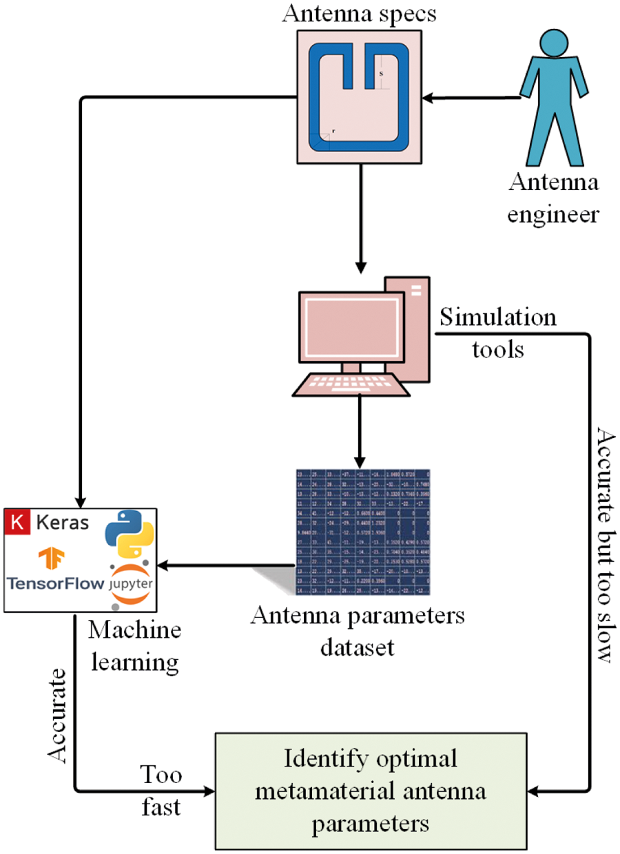
Figure 1: The traditional and proposed design processes of metamaterial antennas
Many applications have been derived from metamaterials. These applications include ultrasensitive sensors [5], wireless power transfer [6], metamaterial lens [7], and metamaterial absorber [8]. These applications emphasize the significance of this kind of material, which attracts many researchers in various disciplines of science. One of these disciplines is the field of engineering microstrip antennas; in specific, metamaterial antennas, which are a special class of antennas that are based on metamaterial to enable them efficiently propagating energy in the free space. On the other hand, the radiation loss and quality factors of microstrip antennas are usually affected by the size of the antenna [9]. For integrated antennas, the good efficiency and low cost represent the main target that researchers try to realize while decreasing the antenna size. One of the main factors that help in realizing this target is the utilization of metamaterial to improve the gain, bandwidth, directivity, and electrical field of small-sized antennas [10].
The effect of metamaterial can be estimated using special software tools used in electromagnetic simulation experiments [11]. One of these tools is the CST microwave studio, which is capable of simulating complex structures. The parameters of antennas such as voltage standing wave ratio (VSWR), gain, bandwidth, and return loss can be estimated from these simulation tools. However, to obtain the optimal values of these parameters, researchers usually use a traditional approach based on trial-and-error to modify/adjust antenna dimensions during the simulation process, which makes this process time-consuming. On the other hand, machine learning offers the best alternative to predict these parameters efficiently and in a very short time when compared with the traditional approach [12].
Machine learning is a widely spread research field that can be easily engaged with many applications in various research fields [13]. The process of building a robust model is considered the main task of machine learning. Once a robust model is built, it can be used in predictions and taking decisions based on the task under consideration. The main advantage of machine learning models is that they are not programmed explicitly, but they can be trained and learned to do their tasks based on a set of training data. Tremendous applications can benefit from the advantages of machine learning. Some of these applications include Forecasting solar radiation [14], Robotics [15], Disease classification [16], and Computer vision [17].
The main role of machine learning in metamaterial simulations is to replace the trial-and-error approach with another quick and accurate approach based on one or more carefully selected machine-learning models for predicting the proper design parameters. The prediction accuracy usually depends on two factors. Firstly, the size of the dataset used in training the machine learning model. Secondly, the type of machine learning model selected for training. In the literature, many approaches can be used in training machine learning models to learn the parameters of metamaterial antennas. These approaches include, K-nearest neighbors (KNN) [18], support vector machines (SVM) [19], decision trees (DT) [20], and artificial neural networks (ANN) [21]. In addition, two or more machine learning approaches can be combined to form an ensemble model, which can result in an enhanced model. From the methods used to build these ensemble models, weighted average ensemble, bagging, boosting, and average ensemble.
Deep learning is considered one of the most promising types of machine learning modeling approaches [22]. Therefore, researchers in some cases define it as an upgraded version of machine learning. This machine learning approach is widely used in the processing and analyzing data from various domains; such as image retrieval, object detection, and image classification. On the other hand, this approach can also be used in regression tasks. For the tasks of predicting the design parameters of antennas, this approach is not widely addressed, as it usually requires a large dataset to be trained efficiently and to predict design parameters accurately. However, the lack of a large dataset including antenna design parameters is a well-known problem in the field of antenna design using machine learning. In this case, transfer learning comes to the rescue, as it offers pre-trained models, which are already trained on a large dataset from different domains and only need fine-tuning to match the given task.
In this paper, we address the application of deep learning to learn the design parameters of metamaterial antennas. In specific, we propose a deep learning network that can accurately predict the bandwidth of metamaterial antenna. The proposed network consists of six dense layers with rectified linear unit (ReLU) activation functions. To learn and measure the optimal weights of this deep network, a guided whale optimization algorithm is employed. The proposed deep network is compared with four recent machine learning models. These models are support vector machines, decision trees, K-nearest neighbors, and average ensemble models. The conducted experiments show that the results achieved by the proposed deep network are better than those of the other models for predicting the bandwidth of metamaterial antenna accurately.
This paper is organized as follows. Section 2 presents the literature review. The details of the proposed methodology are discussed in Section 3. While Section 4 presents and explains the conducted experiments and the achieved results. Finally, the conclusions and future perspectives are presented in Section 5.
In the literature, many areas extended the models of machine learning. These areas include Solar energy [23], Telecommunication [24], Network security [25], Disease classification [26], and Computer vision [27]. In addition, machine-learning models can be used for either classification or prediction of data points without explicit programming of these tasks. In the literature, there are several algorithms developed for building machine learning models, such as KNN, SVM, ANN, and DT. The most common approach used in the literature for data prediction is ANN, which is inspired by the behavior of the biological nervous system in the human brain. In addition, multi-layer perceptron (MLP) is a type of ANN in which the network consists of multi-layers, and each layer is composed of a set of perceptrons/neurons. MLP usually consists of three layers namely, input, hidden, and output layers. Each layer in MLP consists of a set of artificial neurons, which are connected through a set of weights with the next layer of neurons. During the training process of a neural network, the network weights are adjusted properly to generalize over the validation and test sets. When the number of hidden layers in the MLP network exceeds one, this network is called a deep neural network (DNN).
The studies in the literature that addressed the application of machine learning in general and neural networks in specific are numerous. Authors in [28] employed neural networks to track multiple sources and their arrival angles of a smart antenna. In addition, authors in [29] proposed an approach based on ANN to optimize the design parameters of microstrip antennas to adjust their dimensions. In [30], the authors presented the application of ANN to a dual ring antenna to optimize its bandwidth by replacing the full-wave analysis with the parameter prediction using ANN. Moreover, authors in [31] proposed an approach for predicting the impedance of a broadband antenna by training ANN on the geometrical parameters of this antenna. It can be noted that most studies are based on the traditional ANN and, to the best of our knowledge, there is no relevant study, in the literature, utilized DNN for a similar task, which is considered a significant contribution of the proposed approach in this paper.
On the other hand, support machines are considered one of the most relevant and popular approaches in the literature used in predicting the parameters of microstrip antennas. This approach is based on finding the optimal separating hyperplane between binary classes of a dataset. This hyperplane is used to maximize the margin between classes and thus can decrease the classification and prediction errors [32]. Recently, in the field of communication, SVM becomes a popular approach. Authors in [33] applied SVM in an allocation system that targets reducing the complexity of the required computations in the online antenna. In addition, authors in [34] trained SVM on a dataset collected from a microwave simulator. The objective of that research was to improve the performance of a microstrip patch antenna by predicting its feed section.
Sometimes the performance of machine learning models, that are used separately, is not as promising as expected. Therefore, multiple machine learning models can be integrated and employed in a unified ensemble model to achieve better performance [35]. To realize this ensemble model, the simplest approach is to average the outputs of the trained machine learning models to calculate the final output. In this approach, the strength and weight of each model are equal to each other in calculating the final output. Despite the simplicity of this approach, the achieved results are not as promising as expected, as it deals with all the models equally. Due to this disadvantage, another approach was developed by researchers in the literature that gives weight to each model in a smart version of ensemble modeling. The advantage of this approach is that it gives a high weight to the good model in the ensemble and less weight to the other fair models. Authors in [36,37] presented grouping multiple ANNs in a unified ensemble model that is applied to a circular fractal patch antenna to optimize its design parameters.
On the other hand, deep learning is one of the most promising approaches that becomes very popular in almost all the fields of computer science and engineering and other related fields. This approach is based on the notion of neural networks, but with many hidden layers. This type of machine learning model is well prepared and has a lot of implemented libraries available for training custom models for classifying and predicting data accurately. In the field of communication and antenna parameters optimization, this approach is less widely spread. To the best of our knowledge, there are very few attempts, in the literature, that use deep learning in a similar task. Authors in [38] proposed a metasurface design method based on deep learning. The purpose of that method is to detect the inner rules inside the unit cells of a metasurface design. In addition, authors in [39] presented the application of deep learning in the automatic designing of metasurfaces with a wide frequency range. Therefore, in this paper, we propose the application of this approach in predicting the bandwidth of metamaterial antennas, which can be considered as a significant contribution to the field of designing metamaterial antennas.
In this section, the details of the proposed methodology are presented and discussed. The section starts with presenting the dataset along with an exploratory analysis of the dataset parameters and the preprocessing techniques applied to these parameters. In addition, the proposed deep neural network is presented and analyzed along with the optimization algorithm employed to train the proposed deep neural network.
The overall architecture of the proposed approach is exposed in Fig. 2. As shown in the figure, the process starts with collecting a dataset for metamaterial antenna and recording the design parameters using simulation tools. This dataset is usually prepared just once for training machine learning models. As the dataset may contain invalid or null entries in some records of the design parameters, preprocessing is an essential step that must be performed before training the proposed deep network. After preprocessing is accomplished, the dataset becomes ready to train the deep network by splitting this dataset into the train, validation, and test sets. Once the deep network is trained, it can be used for predicting the optimal values of the antenna parameters; in our case, it is used to predict the bandwidth of the metamaterial antenna.
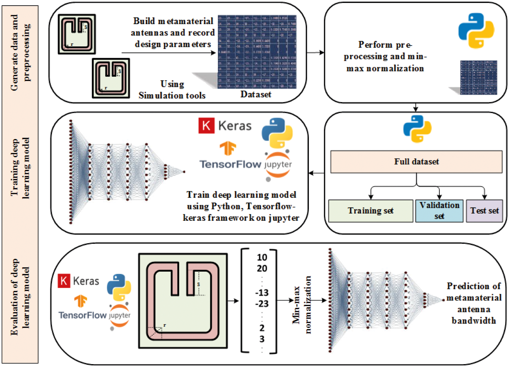
Figure 2: The architecture of the proposed approach
Fig. 3 depicts the Split Ring Resonator (SRR) structure, which is described by the dataset employed in this research. The formulation of SRR consists of two rings with a gap between them. The significance of SRR is that it helps reduce the mutual coupling of the metamaterial antenna and improves its bandwidth [40].
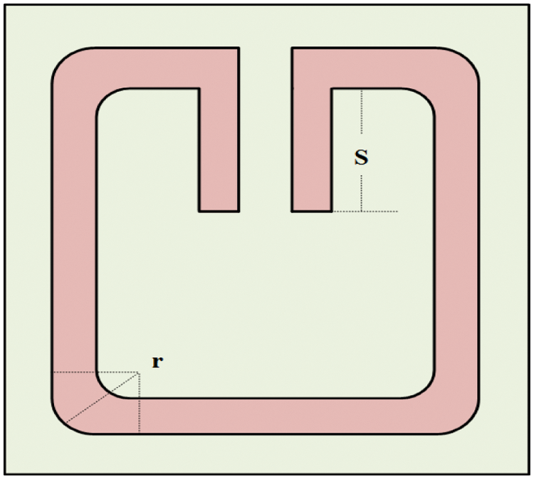
Figure 3: Split-ring resonator shape
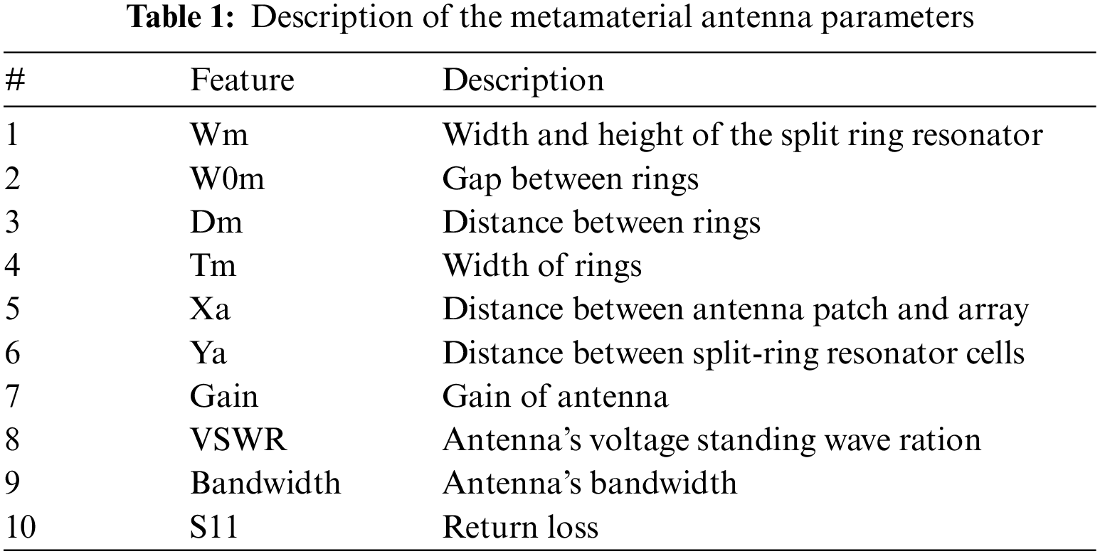
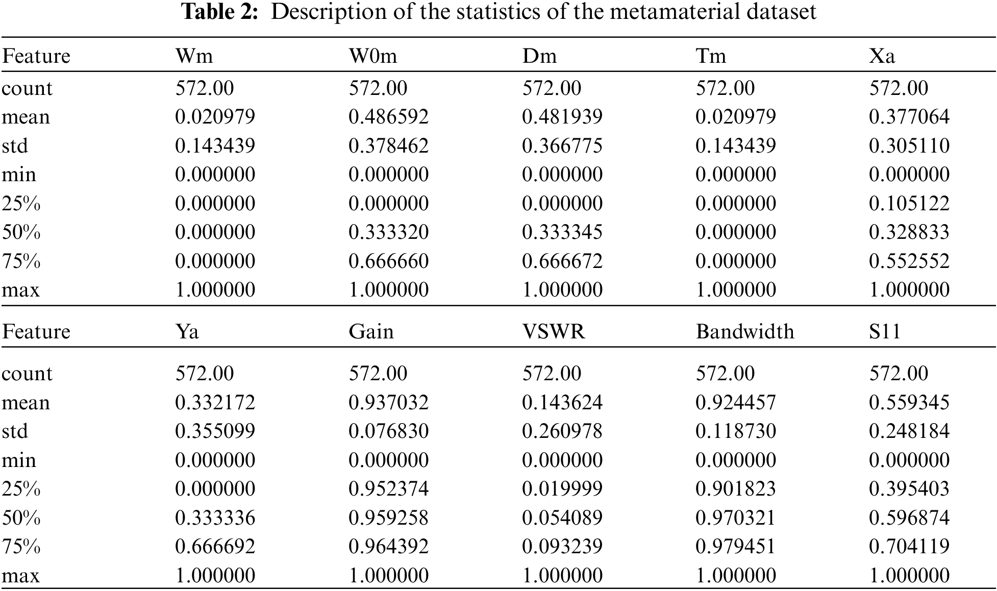
This research employs a dataset consisting of 10 features used to describe the design parameters of a metamaterial antenna. This dataset is available on Kaggle [41] in a tabular form consisting of set rows and columns. The number of rows/records in this dataset is 572, and the number of columns/parameters is 10, namely width and height of the split ring resonator, the gap between rings, the distance between rings, the width of the rings, the distance between antenna patch and array, the distance between split-ring resonator cells in the array, antenna gain, voltage standing wave ratio, bandwidth, and return loss. These parameters along with the corresponding symbols are shown in Tab. 1. In this research, we utilized 9 of these parameters to predict the bandwidth of the metamaterial antenna.
To analyze the given dataset, Fig. 4 depicts the correlation matrix that measures the correlation among the features of the dataset. As shown in this figure, it can be noted that the correlation between the bandwidth and both Ya and Xa is high. However, the bandwidth is less correlated with Wm and Tm. To deeply investigate the behavior of the dataset features, Fig. 5 shows the histogram of each feature along with the Pearson correlation coefficients that measure the linear relationship between the dataset features. The values of these correlation coefficients range from −1 to +1; where values closer to +1 refer to high correlation, whereas the value 0 refers to no correlation. On the other hand, the positive values of the Pearson correlation coefficient indicate that as the values of the features on the X-axis increase, the values of the corresponding features on the Y-axis also increase. However, the negative correlation values indicate that when the values of the X-axis increase, the values on the Y-axis decrease. Moreover, to study the responsibility of the dataset features for the variance, principal component analysis (PCA) is applied. The results of this analysis showed that 17.21% of the variance in the dataset is due to the changes in the values of the feature Ya, and 15.3% of the variance is due to the changes that occurred in the values of W0m. In addition, 13.21% of the variance is due to the changes in the values of the distances between rings [42].

Figure 4: Correlation measure among the design parameters of metamaterial antenna

Figure 5: Histograms and Pearson coefficients of the parameters of the metamaterial antenna dataset
To apply machine-learning techniques to the given dataset, a set of preprocessing tasks is necessary to be applied first. The first task is to handle the null values in the dataset. This task is realized by replacing each null value with the average of the preceding and succeeding not-null values. In addition, the ranges of the values of the dataset features usually affect the performance of machine learning techniques, thus the higher values of these features will dominate the calculations of machine learning techniques and might bias the operation of machine learning to these features over other features of small values.
The second task in the preprocessing stage is to scale and normalize all the features in the dataset. This allows machine learning to treat these features equally as they lay in the same range of values. This task is achieved in this research by utilizing the min-max scalar to scale the features and make them reside in the range from 0 to 1. The equation used to implement this task is presented in the following.
where
The proposed deep neural network consists of 6 dense layers; where each layer is fully connected with all the neurons of the next layer. The activation function used for the neurons in each layer is ReLU. The input layer consists of only 9 receptors to receive the 9 parameters of the metamaterial antenna. These 9 receptors are fully connected to the first layer in the network that consists of 200 neurons. Once the deep network is constructed, the network becomes ready to be trained based on the given dataset.
To show the full connectivity of the layers in a deep network, Fig. 6 depicts a sample structure of a fully connected network. On the other hand, the number of neurons in each hidden layer in the proposed deep network is shown in Tab. 3, in the column named Output Shape. In addition, Fig. 7 presents the internal structure of the artificial neuron. From this figure, the output of the neuron is specified by the following equation.
where ∅ denotes the activation function. In this research, we adopted the ReLU activation function for all neurons. Wi refers to the connection weights, Xi is the input values, and bi is the neuron bias value.

Figure 6: Structure of a sample deep neural network consisting of two hidden layers
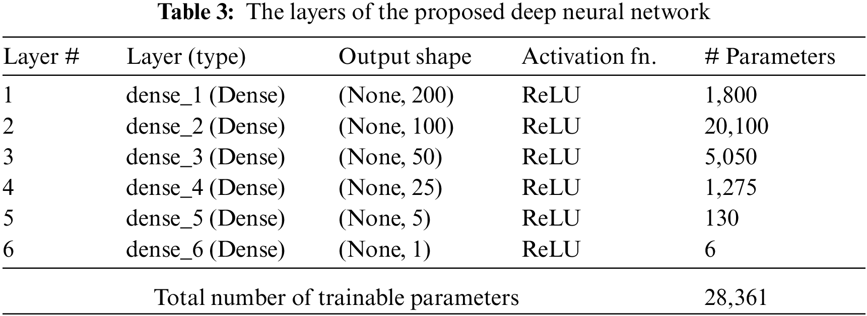

Figure 7: The internal structure of a single artificial neuron
3.4 Guided Whale Optimization Algorithm
The parameters of the proposed deep network (weights and biases) are optimized using the recently published guided whale optimization algorithm (Guided WOA) [26]. This algorithm is based on the foraging behavior of whales that force their prey to surface in a spiral loop to be easily trapped. To find the best parameters using Guided WOA, the search strategy can move directly to this solution by allowing the main whale to follow three other random whales; which effectively improves the exploration performance of this algorithm. This behavior is realized using the following equation.
where the three random whales are denoted by
where t refers to the iteration number, and the maximum number of iterations is denoted by
To find the best set of parameters, a random fractal sample is selected as shown in Fig. 8. Then statistical fractal search is applied to utilize the diffusion by applying two kinds of updating processes. The diffusion process is depicted in a graphical form for a solution in this figure. To improve the exploration, based on the statistical fractal search and its diffusion procedure, a series of random walks around the best solution can be created. This increases the exploration capability of the Guided WOA using this diffusion process for getting the best solution.

Figure 8: Diffusion around the optimal parameters using random fractal sample [26]
To validate the efficiency of the proposed approach, the dataset is divided into three subsets namely, train, validation, and test sets. The ratio of the training subset is 80% and the test subset is 20%, whereas the validation subset is 25% of the training subset. The training of the proposed deep network is performed by initializing the network parameters using random values. Then the guided WOA is applied to find the best values of these parameters through a set of iterations. During the training process, the network tries to learn the prediction of the antenna bandwidth. The measurement of the performance of the trained network is performed in terms of the mean square error (MSE) metric. This metric is calculated as follows.
where
The progress of the training and validation losses is shown in Fig. 9. As shown in the figure, the network could learn the accurate prediction of the bandwidth values from the train set after a few iterations as the loss values approach zero after the first 50 iterations. After training the deep network, the test set is used to evaluate the robustness of the trained model. Fig. 10 shows the prediction of the bandwidth of the test set vs. the actual bandwidth. In this figure, the values of the predicted and actual bandwidths are too close to each other, which indicates the capability of the trained model to achieve accurate predictions of the antenna bandwidth.

Figure 9: Progress of the loss measure during the training process

Figure 10: Actual and predicted bandwidth values
On the other hand, more statistical metrics have been measured to emphasize the superiority of the proposed approach. Fig. 11 presents four other measures of the model performance. The top left sub-figure presents the mapping between the predicted and actual bandwidths, which shows that the predicted values are highly fitted with the actual values. In addition, the residuals vs. actual plots are shown in the top right sub-figure. In this sub-figure, the red circle refers to the region where the predicted values achieve residuals close to zero, which indicates that the predicted values are accurate.

Figure 11: Statistics measuring the performance of the proposed approach
In addition, the partial regression plots are shown in the two sub-figures at the bottom of Fig. 11. These sub-figures present the mapping between the expectations of the actual vs. the predicted values of the test set. From these sub-figures, there is a linear mapping between both of these values, which indicates the better performance of the proposed model.
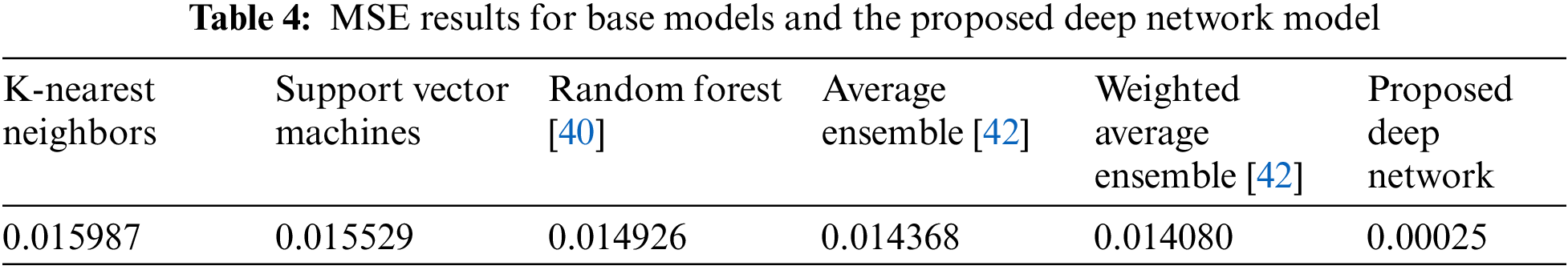
Moreover, Tab. 4 presents a comparison between the values of MSE achieved by the proposed approach and a set of other competing approaches. As shown in the table, the proposed approach could achieve the smallest MSE value among them, which reflects the superiority of the proposed deep network in predicting the values of metamaterial antenna bandwidth.
In this paper, we proposed a new approach based on a deep neural network for predicting the parameters of metamaterial antennas. The proposed approach can accurately predict the bandwidth of metamaterial antennas based on a set of design parameters. In this approach, a deep neural network has been developed and trained using the recently emerged guided whale optimization algorithm. After a few training iterations, the model became capable of predicting the bandwidth with high precision. To validate the superiority of the proposed approach, four baseline models were incorporated in the conducted experiments. Experimental results show that the proposed approach is robust and can achieve the minimum mean square error among all the other competing approaches. In addition, statistical analysis is performed to show the effectiveness of the proposed approach. In this analysis, the actual and predicted bandwidths were investigated to confirm and emphasize the robustness of the proposed approach. The future perspectives of this research include applying the proposed approach to more types of microstrip antennas and harnessing it with ensemble models to achieve better results in predicting the parameters of antenna design parameters.
Acknowledgement: The authors extend their appreciation to the Deputyship for Research & Innovation, Ministry of Education in Saudi Arabia for funding this research work through the Project Number (IFP2021-033).
Funding Statement: The authors received funding for this study from the Deputyship for Research & Innovation, Ministry of Education in Saudi Arabia for funding this research work through the Project Number (IFP2021-033).
Conflicts of Interest: The authors declare that they have no conflicts of interest to report regarding the present study.
1. J. Suganthi, T. Kavitha and V. Ravindra, “Survey on metamaterial antennas,” IOP Conference Series: Materials Science and Engineering, vol. 1070, no. 1, pp. 12086, 2021. [Google Scholar]
2. M. Alibakhshikenari, B. Virdee, L. Azpilicueta, M. Naser-Moghadasi, M. Akinsolu et al., “A comprehensive survey of metamaterial transmission-line based antennas: Design, challenges, and applications,” IEEE Access, vol. 8, pp. 144778–144808, 2020. [Google Scholar]
3. H. Misilmani and T. Naous, “Machine learning in antenna design: An overview on machine learning concept and algorithms,” in Int. Conf. on High-Performance Computing & Simulation (HPCS), Dublin, Ireland, pp. 600–607, 2019. [Google Scholar]
4. W. Naktong, A. Ruengwaree, N. Fhafhiem and P. Krachodnok, “Resonator rectenna design based on metamaterials for low-RF energy harvesting,” Computers, Materials & Continua, vol. 68, no. 2, pp. 1731–1750, 2021. [Google Scholar]
5. X. Chen and W. Fan, “Ultrasensitive terahertz metamaterial sensor based on spoof surface plasmon,” Scientific Reports, vol. 7, no. 1, pp. 1–8, 2017. [Google Scholar]
6. K. Sun, R. Fan, X. Zhang, Z. Zhang, Z. Shi et al., “An overview of metamaterials and their achievements in wireless power transfer,” Journal of Materials Chemistry, vol. 6, no. 12, pp. 2925–2943, 2018. [Google Scholar]
7. N. Kundtz and D. R. Smith, “Extreme-angle broadband metamaterial lens,” Nature Materials, vol. 9, no. 2, pp. 129–132, 2010. [Google Scholar]
8. N. Landy, S. Sajuyigbe, J. Mock, D. Smith, W. Padilla et al., “Perfect metamaterial absorber,” Physical Review Letters, vol. 100, no. 20, pp. 207402, 2008. [Google Scholar]
9. Y. Dong and T. Itoh, “Metamaterial-based antennas,” Proc. of the IEEE, vol. 100, no. 7, pp. 2271–2285, 2012. [Google Scholar]
10. H. Askari, N. Hussain, D. Choi, M. Sufian, A. Abbas et al., “An AMC-based circularly polarized antenna for 5G sub-6 GHz communications,” Computers, Materials & Continua, vol. 69, no. 3, pp. 2997–3013, 2021. [Google Scholar]
11. G. Geetharamani and T. Aathmanesan, “Design of metamaterial antenna for 2.4 GHz WiFi applications,” Wireless Personal Communications, vol. 113, no. 4, pp. 2289–2300, 2020. [Google Scholar]
12. M. Saputra, S. Sulistiyanti, S. Purwiyanti and U. Murdika, “Design of prototype measuring motor vehicles velocity using hall effect sensor series A-1302 based on arduino mega 2560,” in 2nd Int. Conf. on Industrial Electrical and Electronics (ICIEE), Lombok, Indonesia, pp. 66–69, 2020. [Google Scholar]
13. M. Jordan and T. Mitchell, “Machine learning: Trends, perspectives, and prospects,” Science, vol. 349, no. 6245, pp. 255–260, 2015. [Google Scholar]
14. R. Al-Hajj, A. Assi and M. Fouad, “Stacking-based ensemble of support vector regressors for one-day ahead solar irradiance prediction,” in 8th Int. Conf. on Renewable Energy Research and Applications (ICRERA), Brasov, Romania, pp. 428–433, 2019. [Google Scholar]
15. A. I. Karoly, P. Galambos, J. Kuti and I. J. Rudas, “Deep learning in robotics: Survey on model structures and training strategies,” IEEE Transactions on Systems, Man, and Cybernetics, vol. 51, no. 1, pp. 266–279, 2021. [Google Scholar]
16. E. El-Kenawy, S. Mirjalili, A. Ibrahim, M. Alrahmawy, M. El-Said, R. Zaki et al., “Advanced Meta-Heuristics, Convolutional Neural Networks, and Feature Selectors for Efficient COVID-19 X-Ray Chest Image Classification,” IEEE Access, vol. 9, pp. 36019–36037, 2021. [Google Scholar]
17. A. Ibrahim, S. Tominaga and T. Horiuchi, “Spectral imaging method for material classification and inspection of printed circuit boards,” Optical Engineering, vol. 49, no. 5, pp. 57201, 2010. [Google Scholar]
18. N. Bhatia, “Survey of nearest neighbor techniques,” International Journal of Computer Science and Information Security, vol. 8, no. 2, pp. 302–305, 2010. [Google Scholar]
19. W. Noble, “What is a support vector machine?,” Nature Biotechnology, vol. 24, no. 12, pp. 1565–1567, 2006. [Google Scholar]
20. A. Myles, R. Feudale, Y. Liu, N. Woody and S. Brown, “An introduction to decision tree modeling,” Journal of the Chemometrics Society, vol. 18, no. 6, pp. 275–285, 2004. [Google Scholar]
21. B. Yegnanarayana, “Artificial neural networks,” in PHI Learning Pvt. Ltd, Delhi, India, 2009. [Google Scholar]
22. T. Badriyah, D. Santoso and I. Syarif, “Deep learning algorithm for data classification with hyperparameter optimization method,” in Int. Conf. of Computer and Informatics Engineering (IC2IE), Bogor, Indonesia, pp. 1–8, 2019. [Google Scholar]
23. R. Al-Hajj, A. Assi and M. Fouad, “A predictive evaluation of global solar radiation using recurrent neural models and weather data,” in IEEE 6th Int. Conf. on Renewable Energy Research and Applications (ICRERA), San Diego, CA, USA, pp. 195–199, 2017. [Google Scholar]
24. M. Svensson and S. JoakiM, “Machine-learning technologies in telecommunications,” Ericsson Review, vol. 3, pp. 29–33, 2008. [Google Scholar]
25. M. Amrollahi, S. Hadayeghparast, H. Karimipour, F. Derakhshan and G. Srivastava, “Enhancing network security via machine learning: Opportunities and challenges,” in Handbook of Big Data Privacy, Cham: Springer Nature Switzerland: Springer, pp. 165–189, 2020. [Google Scholar]
26. E. El-Kenawy, A. Ibrahim, S. Mirjalili, M. Eid and S. Hussein, “Novel feature selection and voting classifier algorithms for COVID-19 classification in CT images,” IEEE Access, vol. 8, pp. 179317–179335, 2020. [Google Scholar]
27. T. Gaber, A. Tharwat, A. Ibrahim, V. Snael and A. E. Hassanien, “Human thermal face recognition based on random linear oracle (RLO) ensembles,” in Int. Conf. on Intelligent Networking and Collaborative Systems, Taipei, Taiwan, pp. 91–98, 2015. [Google Scholar]
28. A. El Zooghby, C. Christodoulou and M. Georgiopoulos, “A neural network-based smart antenna for multiple source tracking,” IEEE Transactions on Antennas and Propagation, vol. 48, no. 5, pp. 768–776, 2000. [Google Scholar]
29. U. Ozkaya and L. Seyfi, “Dimension optimization of microstrip patch antenna in X/Ku band via artificial neural network,” In Procedia-Social and Behavioral Sciences, vol. 195, pp. 2520–2526, 2015. [Google Scholar]
30. L. H. Manh, F. Grimaccia, M. Mussetta and R. Zich, “Optimization of a dual ring antenna by means of artificial neural network,” Progress in Electromagnetics Research, vol. 58, pp. 59–69, 2014. [Google Scholar]
31. Y. Kim, S. Keely, J. Ghosh and H. Ling, “Application of artificial neural networks to broadband antenna design based on a parametric frequency model,” IEEE Transactions on Antennas and Propagation, vol. 55, no. 3, pp. 669–674, 2007. [Google Scholar]
32. J. Nayak, B. Naik and H. Behera, “A comprehensive survey on support vector machine in data mining tasks: Applications & challenges,” Journal of Database Theory and Application, vol. 8, no. 1, pp. 169–186, 2015. [Google Scholar]
33. H. Lin, W. Shin and J. Joung, “Support vector machine-based transmit antenna allocation for multiuser communication systems,” Entropy, vol. 21, no. 5, pp. 471, 2019. [Google Scholar]
34. S. lker, “Support vector regression analysis for the design of feed in a rectangular patch antenna,” in 3rd Int. Symp. on Multidisciplinary Studies and Innovative Technologies (ISMSIT), Ankara, Turkey, pp. 1–3, 2019. [Google Scholar]
35. R. Al-Hajj, A. Assi and M. Fouad, “Short-term prediction of global solar radiation energy using weather data and machine learning ensembles: A comparative study,” Journal of Solar Energy Engineering, vol. 143, no. 5, pp. 51003, 2021. [Google Scholar]
36. B. Dhaliwal and S. Pattnaik, “Development of PSO-ANN ensemble hybrid algorithm and its application in compact crown circular fractal patch antenna design,” Wireless Personal Communications, vol. 96, no. 1, pp. 135–152, 2017. [Google Scholar]
37. S. Pattnaik, S. Pattnaik and B. Dhaliwal, “Modeling of circular fractal antenna using BFOPSO-based selective ANN ensemble,” International Journal of Numerical Modelling: Electronic Networks, Devices and Fields, vol. 32, no. 3, pp. e2549, 2019. [Google Scholar]
38. T. Qiu, X. Shi, J. Wang, Y. Li, S. Qu et al., “Deep learning: A rapid and efficient route to automatic metasurface design,” Advanced Science, vol. 6, pp. 1900128, 2019. [Google Scholar]
39. F. Ghorbani, S. Beyraghi, J. Shabanpour, H. Oraizi, H. Soleimani et al., “Deep neural network-based automatic metasurface design with a wide frequency range,” Scientific Reports, vol. 11, no. 7102, 2021. [Google Scholar]
40. N. Kurniawati, D. Putri and Y. Ningsih, “Random forest regression for predicting metamaterial antenna parameters,” in Int. Conf. on Industrial Electrical and Electronics, Indonesia, pp. 174–178, 2020. [Google Scholar]
41. R. Machado, Metamaterial Antennas, 2019. [Online]. Available: https://www.kaggle.com/renanmav/metamaterial-antennas. [Accessed: 2021-12-01]. [Google Scholar]
42. A. Ibrahim, H. Abutarboush, A. Mohamed, M. Fouad and E. El-kenawy. “An optimized ensemble model for prediction the bandwidth of metamaterial antenna,” Computers, Materials & Continua, vol. 71, no. 1, pp. 199–213, 2022. [Google Scholar]
 | This work is licensed under a Creative Commons Attribution 4.0 International License, which permits unrestricted use, distribution, and reproduction in any medium, provided the original work is properly cited. |