Computers, Materials & Continua DOI:10.32604/cmc.2022.025741
Article

Hybrid Chaotic Salp Swarm with Crossover Algorithm for Underground Wireless Sensor Networks

Mariem Ayedi1,2,*, Walaa H. ElAshmawi3,4 and Esraa Eldesouky1,3

1First Department of Computer Science, College of Computer Engineering and Sciences, Prince Sattam Bin Abdulaziz University, Al-Kharj, 11942, Saudi Arabia
2MEDIATRON Lab., SUP'COM, Carthage University, Tunis, 2083, Tunisia
3Department of Computer Science, Faculty of Computers and Informatics, Suez Canal University, Ismailia, 41522, Egypt
4Faculty of Computer Science, Misr International University, Cairo, Egypt
*Corresponding Author: Mariem Ayedi. Email: m.ayedi@psau.edu.sa
Received: 03 December 2021; Accepted: 17 January 2022

Abstract: Resource management in Underground Wireless Sensor Networks (UWSNs) is one of the pillars to extend the network lifetime. An intriguing design goal for such networks is to achieve balanced energy and spectral resource utilization. This paper focuses on optimizing the resource efficiency in UWSNs where underground relay nodes amplify and forward sensed data, received from the buried source nodes through a lossy soil medium, to the aboveground base station. A new algorithm called the Hybrid Chaotic Salp Swarm and Crossover (HCSSC) algorithm is proposed to obtain the optimal source and relay transmission powers to maximize the network resource efficiency. The proposed algorithm improves the standard Salp Swarm Algorithm (SSA) by considering a chaotic map to initialize the population along with performing the crossover technique in the position updates of salps. Through experimental results, the HCSSC algorithm proves its outstanding superiority to the standard SSA for resource efficiency optimization. Hence, the network's lifetime is prolonged. Indeed, the proposed algorithm achieves an improvement performance of 23.6% and 20.4% for the resource efficiency and average remaining relay battery per transmission, respectively. Furthermore, simulation results demonstrate that the HCSSC algorithm proves its efficacy in the case of both equal and different node battery capacities.

Keywords: Underground wireless sensor networks; resource efficiency; chaotic theory; crossover algorithm; salp swarm algorithm

1  Introduction

With the precipitous growth of microelectronics and sensing technologies, Wireless Sensor Networks (WSNs) have been categorized as an intense research arena. The outstanding privileges of such networks, including their easy configuration, mobility, and flexibility, lead to their deployment in many environments. UWSNs are an important extension of WSNs applications for use in the underground world. These underground networks have a broad range of applications including tracking coal mining facilities, soil monitoring, and gas/oil pipeline control. In such networks, buried sensors continuously collect sensitive data regarding the sensed environment and forward it to the base station [1]. However, the limited communication range and the energy constraints along with the complex and unpredictable conditions of the underground medium are the primary challenges of UWSNs. Thus, the role of relay nodes is vital in UWSNs because they represent a promising method for achieving high bandwidth and expanding network coverage [2]. In UWSNs, communications among nodes come in three distinct channels: UnderGround-to-AboveGround (UG2AG), UnderGround-to-UnderGround (UG2UG), and AboveGround-to-UnderGround (AG2UG) [3]. The UG2AG channel connection is mainly used to transmit sensed data from buried sensors to relay nodes or aboveground base stations [3–5]. Relay node deployment has been studied in UWSNs [5–8]. In [5], an underground coal mine was divided into separate regions and addressed optimal relay node placement to support robust coverage of the network. In [6], Wu targeted controlling the amount of energy used by underground sensors to map water pipelines through optimal relay placement. In the same way, the optimum relay node location was debated for the goal of extending the network's duration subjected to reducing the load balance and the number of relays [7]. In [8], two approximation algorithms for relay node deployment and assignment to sensor nodes were introduced to reduce transmission loss among nodes. Since high throughput and capacity are critically constrained by nodes energy consumption, research work in WSN focus recently on studying the trade-off between spectral efficiency and energy efficiency metrics called the resource efficiency [9–12]. The primary objective is to jointly evaluate the efficient use of a limited frequency spectrum along with energy consumption. In UWSNs, this problem was first addressed in [13], where optimal powers used by underground sources and relay nodes for data forwarding to an aboveground base station were computed to maximize the energy and spectral efficiency tradeoff. The work [13] proposes a power allocation algorithm that utilizes the Salp Swarm Algorithm (SSA) [14] to solve the considered problem since the swarm intelligence models are interesting for various computer science fields [15,16]. The SSA is suggested in [14] as a recent metaheuristic algorithm which outperforms many other metaheuristic algorithms through tests on 19 different benchmark functions. In nearby research works, SSA proves its efficiency in node localization optimization in WSN [17,18], energy consumption and lifetime optimization in WSN [19]. The work [13] proves that the SSA-based scheme offers a better resource efficiency, given similar bandwidth and battery cost resources, compared with the traditional UWSN scheme. In this paper, we propose to further enhance the resource efficiency of the UWSN considered in [13] by modifying and improving the SSA. A novel algorithm called Hybrid Chaotic Salp Swarm with Crossover (HCSSC) is proposed to determine the optimal powers required by the source and relay nodes that enhance the network resource efficiency considering the initial nodes’ battery capacities. The proposed algorithm uses chaos theory [20] to generate feasible initial solutions. This can enhance the diversity of solutions due to the randomness and dynamic features of the chaos. Moreover, to compute the final optimal solution, a uniform crossover operator [21,22] is integrated in the exploration phase of the optimization algorithm. This leads to accelerated algorithm convergence due to the wide exploration of the search space. The proposed power optimization scheme is evaluated in terms of its effect on the average relay power and battery remaining per transmission. Since the relay node can have a higher battery capacity than the source node, we propose to study the efficiency of the proposed algorithm under both equal and different node capacities.

The main contributions of this work are listed as follows

1.    A new algorithm called HCSSC algorithm is proposed to improve the standard SSA by considering a logistic chaotic map to initialize the population and integrating the uniform crossover operator in the update of salps positions.

2.    The resource efficiency performance is ameliorated compared to that obtained in the work [13].

3.    The average consumed relay power per transmission is minimized and the average remaining relay battery per transmission is maximized.

4.    The efficiency of the proposed algorithm is proved in case of both equal and different node batteries capacities.

This paper is structured as follows. In Section 2, the UWSN system model is presented and the considered problem is formulated. In Section 3, the proposed HCSSC algorithm is detailed. In Section 4, the experimental results and performance analysis are discussed, and finally, Section 5 concludes the paper.

2  System Model and Problem Formulation

The considered UWSN model consists of sensor source node S that gathers and forwards sensory data to an aboveground base station B through a half-duplex Amplify-and-Forward (AF) relay node R. The communication link between S and R is an UG2UG link, whereas the communication link between   R  and  B is an UG2AG link. The mathematical expressions of the path losses for UG2UG and UG2AG, the communication mechanism among nodes, and the optimization problem under consideration are described in this section.

2.1 UG2UG and UG2AG Channel Model

Both source and relay nodes are buried in the soil in UWSNs. Here, the sensor nodes are buried deeper than the relay nodes according to the ground surface. In Fig. 1, a two-dimensional plane represents UWSN deployment where the nodes distances in the plane using Cartesian coordinates defined on the x and y axes with origin O. The base station is positioned at the origin of x-axis whereas the ground surface is represented as the origin of y-axis. dXG is the node burial depth at positions (xX,yY) for node X∈{S,R}.

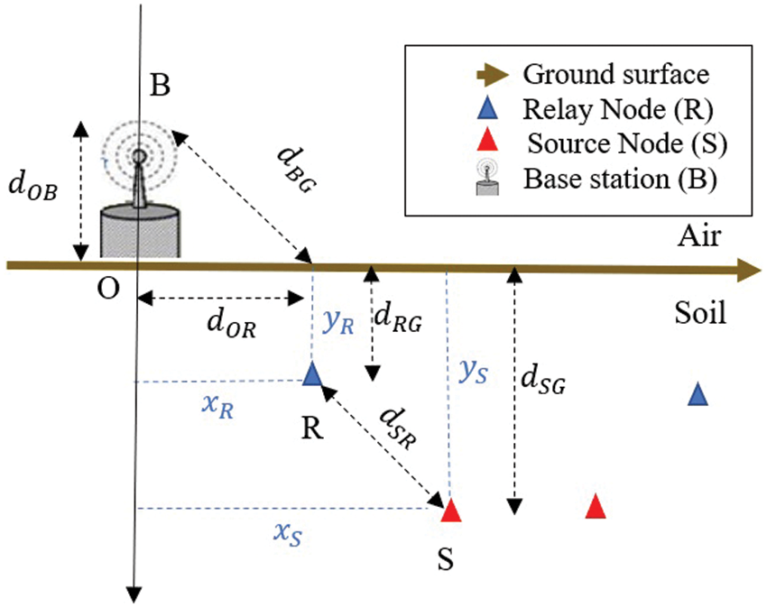
Figure 1: The topology of UWSN

According to [23], the UG2UG path loss LuuSR is defined as

LuuSR=6.4  +20log10(dSR)+20log10(β)+  8.69αdSR−10log10(V)(1)

where dSR=(xS−xR)2+(yS−yR)2 is the distance in metres between S and R. The constants α and β measure the attenuation and phase shifting, respectively. The factor V represents the attenuation of the reflection path obtained when the wave is reflected by the ground surface. Hence, the UG2UG communication results from the propagation of the signal in the reflection path and in the direct path between the two sensors [22]. The authors in [24] utilize the electromagnetic propagation model to provide the detailed expressions the constants α and β. The soil medium dielectric characteristics along with the system operating frequency q, the sand and clay percentages, the bulk density and the Volumetric Water Content constitute the main features that these constants depend on [25]. The soil and air constitute the two media throughout passes the communication between R and B. Yet, there is no refraction loss from under to aboveground transition due to the perpendicular propagation of signal from higher to lower density medium [3,26]. Then, based on [3,26], the path loss LuaRB of the channel between R and B is the result of adding the path losses for both underground and aboveground portions as in Eq. (2)

LuaRB=LuRG+LaGB,(2)

LuRG=6.4+20log10(dRG)+20log10(β)+  8.69αdRG,(2.1)

LaGB,=−147.6  +10ηlog10(dBG)+20log10(q),(2.2)

dBG=dOR2+dOB2,(2.3)

where dOR represents the horizontal distance between R and the origin O, dOB is the height of the aboveground base station B and η is the attenuation coefficient on air [26].

2.2 UWSN System Model

Here, the uplink communication procedure among the trio link is presented. The Time Division Multiple Access (TDMA) scheme is considered to mitigate the signal interference. Each node X∈{S,R} has a limited battery with power capacity CX. At each packet transmission, t, node X consumes a power PXt∈[PXmin,PXmax]. The communication process at each transmission t∈[1,τ] needs two phases.

In the first phase, the source node S transmits a data packet dt to the relay node R. The resulting received signal yRt at R is given by

yRt=PSthSRtdt+nRt(3)

such that hSRt represents the gain of the UG2UG channel between the two nodes S and R, which obeys to the Rayleigh distribution [23] with the underground path loss LuuSR calculated in Eq. (1) and nRt is the zero-mean complex Additive White Gaussian Noise (AWGN) vector with variance N0. Hence, the Signal-to-Noise Ratio (SNR) between S and R designated by ΓSRt, resulting of the communication between S and R at transmission t, is as follows

ΓSRt=PSt|hSRt|2bN0(4)

Where b denotes the channel bandwidth in Hz, which is equal to the operating frequency q when TDMA is applied. In the second phase, the signal yRt is amplified and forwarded by R to B. Consequently, the received signal yBt at B is calculated as follows.

yBt=AftPRthRBtyRt+nBt(5)

With hRBt is the UG2AG Rayleigh distributed channel between R and B [23] with the underground path loss LuaRB calculated in Eq. (2),nBt is the zero-mean complex AWGN vector and Aft=1PSt|hSRt|2+N0 is the amplification factor. Thus, the SNR, denoted by ΓRBt, of the transmission between R and B is computed as follows.

ΓRBt=Aft2PRtPSt|hRBt|2|hSRt|2bN0(Aft2PRt|hRBt|2+1)(6)

With respect to Eqs. (4) and (6), the total SNR Γtott and the maximum data rate Rtott for the trio link are given respectively by

Γtott=ΓSRtΓRBt1+ΓSRt+ΓRBt(7)

Rtott=blog2(1+Γtott)(8)

2.3 Problem Formulation

The overall paper objective is to determine the power allocation vector P=[PSt,PRt] allowing an efficient balance between two competing metrics: the energy efficiency EEt and spectral efficiency SEt at each transmission t. Indeed, EEt. is the total bits generated per unit energy whereas SEt represents the total delivered bits per unit bandwidth of link (S−R−B) at transmission t. Their expressions are respectively as follows

EEt=RtottPSt+PRt,(9)

SEt=Rtottb(10)

As discussed in [9], the resource efficiency metric REt is capable to exploit the trade-off between EEt and SEt. It is given by

REt=EEt+ωSEt(11)

where the weighted factor ω is computed as ω=ω¯bPtot, with ω¯ is a constant and Ptot=PSmax+PRmax is the total power budget allocated to the link (S−R−B) at each transmission. Since, SEt is practically smaller than EEt, this weighted factor ω is utilized to achieve the balance between EEt and SEt. In fact, it solves the inconsistence of adding two metrics with different units since the unit of EEt is bits/Joule while the unit of SEt is bits/s/Hz. Then, the unit of REt is equivalent to EEt which is still bits/Joule. Besides, maximizing REt is simply maximizing EEt if ω¯=0 and SEt if ω¯=∞. The selection of this constant value in the UWSN model is described in [13].

For each node X, optimizing the power PXt at each transmission t is a mandatory requirement because it depends on the limited battery capacity CX of the buried node, the spent powers for transmissions [PX1,…,PXt−1] and the allowed power limitation range at each transmission [PXmin,PXmax]. Then, the proposed optimization problem is stated as

MaximizeRE=∑t=1τREt(12)

Subject to (∑t=1τ⁡PXt)≤CX,

where PXt∈[PXmin,PXmax] for X∈[S,R].

In Eq. (12), the maximization problem presented is considered a NP-hard problem that requires an efficient optimization algorithm to solve it. Therefore, a hybrid meta-heuristic algorithm based on SSA is proposed to obtain optimal values of nodes powers considering the resource efficiency RE to be maximized.

3  The Proposed HCSSC for Resource Efficiency

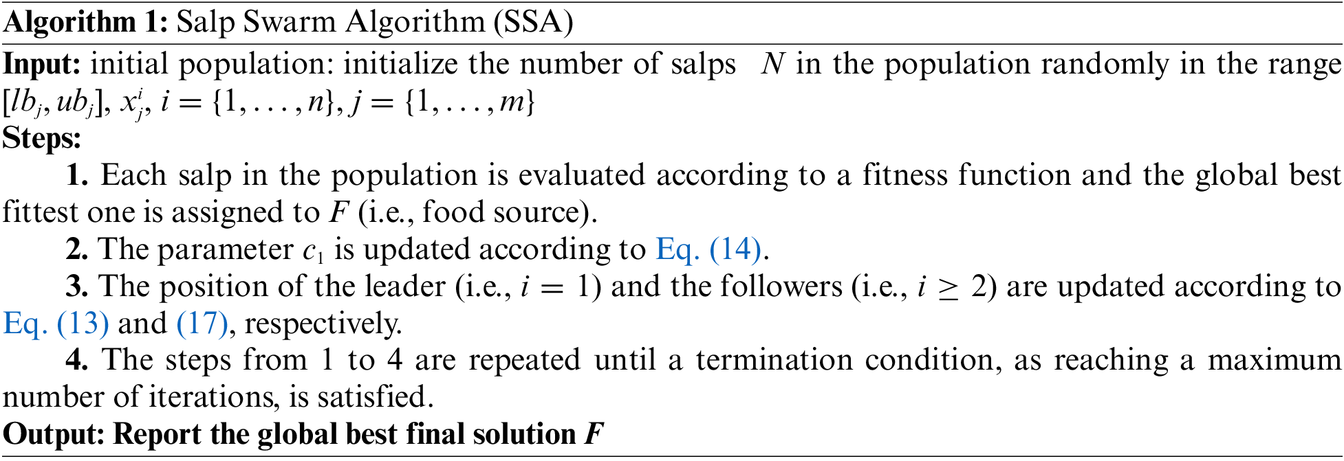
In this section, the main structure of the standard Salp Swarm Algorithm (SSA) is first reviewed. Then, the detailed steps of the proposed Hybrid Chaotic Salp Swarm with Crossover (HCSSC) scheme for maximizing the resource efficiency in the considered UWSN are addressed.

3.1 Salp Swarm Algorithm (SSA)

The Salp Swarm Algorithm (SSA) is one of the recent swam algorithms proposed in 2017 [14] and widely used in solving many optimization problems [27,28]. SSA emulates the motion of Salpidae that have a transparent barrel-shaped body and live-in deep oceans [29]. Salps are organized in a form of swarm called salp chain. Mathematically, the salp chain is divided into two groups: leader (i.e., the first salp of the chain and followers (i.e., the remaining salps of the chain which follow the leader). Researchers viewed that their searching for food is an indicator to their behavior [30].

The leader in the swarm updates its position relative to the food source F according to Eq. (13)

xj1={Fj+c1((ubj−lbj)c2+lbj)c3≥0Fj−c1((ubj−lbj)c2+lbj)c3<0(13)

Where xj1 is the position of the leader in the jth dimension, lbj and ubj are the lower and the upper bound of the jth dimension, respectively, and Fj is the position of food source in the jth dimension. The parameter c1 balances the scale between exploration and exploitation and is computed according to Eq. (14). The coefficients c2 and c3 are random numbers between [−1, 1]. Also, c3 determines the direction of moving the leader towards a positive infinity or negative infinity.

c1=2e−(4lL)2(14)

where l is the current iteration and L is the maximum number of iterations.

The remaining of the salps in the chain (i.e., followers) update their positions based on the Newton's law of motion as in Eq. (15)

xji=12at2c+v0t∀i≥2(15)

wherea=vfinalv0andv=x−x0t(16)

With xj1 is the ith salp in the jth dimension,t is the time,v0 is the initial speed.

In the optimization problems, the time is considered as an iteration where the conflict between iterations is equal to 1 and v0 is set to 0. Then, Eq. (15) can be reformulated in Eq. (17) for updating the positions of followers.

xji=12(xji+xji−1)∀i≥2(17)

While the global optimal solution of any optimization problem is unknown, the best solution can be obtained by moving the leader, followed by the followers, towards the food source. As a result, the salp chain moves towards the global optimum. The overall steps of the SSA are described below.

3.2 Hybrid Chaotic Salp Swarm with Crossover (HCSSC) Algorithm for RE

This subsection discusses the main steps of the proposed HCSSC algorithm to find the optimal source and relay nodes powers for maximizing the resource efficiency REt at each packet transmission t in the UWSN. Assuming that B has perfect Channel State Information (CSI) awareness, the proposed HCSSC algorithm is implemented at B which will send the obtained powers values to source and relay nodes prior to their packets’ transmissions. The hybrid algorithm uses a logistic chaotic map to generate a feasible initial population at random. Furthermore, improving the solution during the number of iterations through the uniform crossover operator and chaotic map can guarantee that the optimal solution is the final solution. The steps of the proposed HCSSC are discussed in detail as follows.

3.2.1 Initial Population

Each salp (i.e.,xi, i={1,…,n}) in the HCSSC population N corresponds to a possible solution for the resource efficiency optimization problem. Moreover, each salp consists of many variables (i.e.,var(j), j={1,…,m}) that affect the optimization of the resource efficiency as shown in Fig. 2. This paper considers a salp x consists of two variables which are PS and PR. An illustrative example of a salp x is shown in Fig. 3. The value for each variable can be generated within the lower PXmin and upper PXmax bounds, respectively.

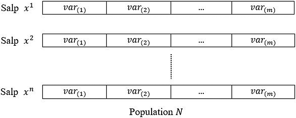
Figure 2: HCSSC population

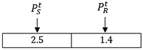
Figure 3: An illustrative example of salp x

The diversity of the initial population has a great impact on spreading effectively in the search space. Therefore, for generating an effective initial population, a chaotic map is used in the proposed algorithm. One of the simplest maps is the logistic map that appears in the nonlinear dynamics of a biological population that evidences the chaotic behavior [31] and it is represented mathematically by Eq. (18).

ck+1=rck(1−ck)(18)

where ck is the chaotic value at each independent run k (i.e.,ck∈(0,1)), r is the growth rate that controls the behavior of chaotic value at a certain time (r=4). To be more specific, the generated random value of resources at any given time (round) is a function of the growth rate parameter and the previous time step's resource's value. Consequently, the initial population N of the proposed HCSSC algorithm is generated according to the following pseudo code.

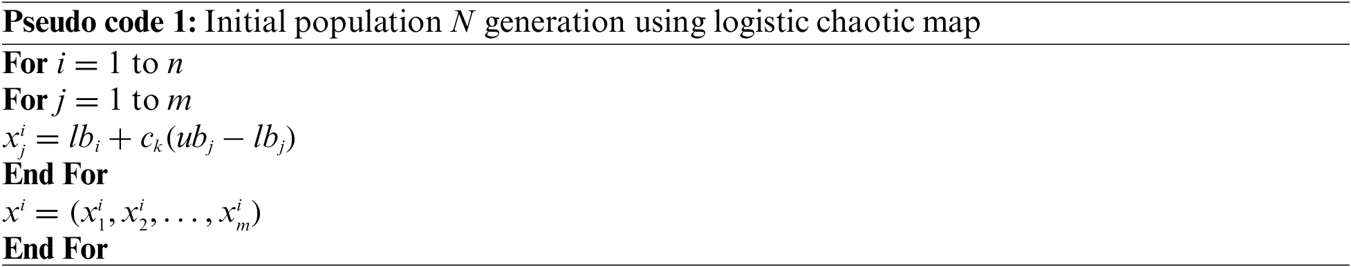
Each variable is bounded within lower and upper values [lbj,ubj], ck is the chaotic sequence that is generated by logistic chaotic map. The integration of chaotic maps with salp swarm algorithm leads to produce a proper distribution through the characteristic of random and stochasticity of chaos.

3.2.2 Evaluation of Salps

The resource efficiency optimization can be modelled as an optimization problem with a maximized objective function. Therefore, each individual (i.e., salp) in the population is evaluated according to Eq. (12) and the fittest one is assigned to F.

3.2.3 Updating Salps

The first salp in the population is called the leader which is responsible for guiding the salp chain and is continuously updating its position towards the direction of the source food. The rest salps in the population are called the followers because they follow the leader in updating their positions. Leader's and followers’ updates are illustrated below.

•   Leader's update

Since the leader updates its position in a positive direction, we ignore the negative direction. Also, the random numbers c2 and c3 are replaced by a chaotic sequences ck1 and ck2 computed according to Eq. (18) while c1 is calculated according to Eq. (14). Thus, Eq. (13) is modified and represented in Eq. (19)

xj1=Fj+c1((ubj−lbj)ck1+lbj)ck2≥0(19)

•   Follower's updates

Each follower xji; i≥2 in the population updates its position based on how far the current position from the best salp's position. To achieve a better follow to the leader, we mate the best individual with the current individual through the uniform crossover [21,32]. The uniform crossover proves its efficiency compared to other crossover operators [20]. An illustrative example of uniform crossover is shown in Fig. 4.

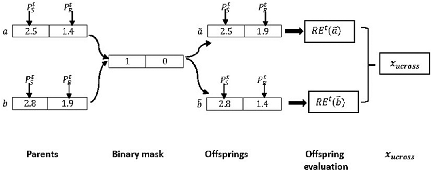
Figure 4: An illustrative example of uniform crossover

In the process of crossover, two parents (a and b) are selected and a binary mask consists of 1/0 digits is generated randomly with the same length of the individual. The result of this operation is generating two offsprings (a~ and b~) based on the corresponding digit in the binary mask. For the first offspring (a~), if the digit in a mask is 1, then the digit it is taken from (a) otherwise from (b). Regarding the generation offspring (b~), the complementary of mask is used. The two obtained offsprings a~ and b~ are considered as two new salps in the population. Each offspring x~∈{a~,b~} is a vector of two variables x~=[PSt,PRt]. Then, the objective function, which is the resource efficiency at each transmission, t, REt of each offspring x~∈{a~,b~} denoted by REt(x~) is evaluated as follows

REt(x~)=REt(PSt,PRt)=EEt(PSt,PRt)+ωSEt(PSt,PRt)(20)

Further, REt(a~) and REt(b~) are compared. If REt(a~)>REt(b~), then, a~ is chosen to be xucross, else, b~ is chosen to be xucross. Therefore, each follower in the salp chain updates its position as follows

xji=12(xucross+xji−1)∀i≥2(21)

3.2.4 Test the Termination Condition

The leader and followers are updating their positions iteratively until reaching a maximum number of iterations. Once the HCSSC algorithm reached the termination condition, the global best salp is returned as the best solution so far for the resource efficiency REt at each packet transmission t. The overall steps of the HCSSC algorithm for optimizing the resource efficiency in UWSN are described in the Fig. 5.

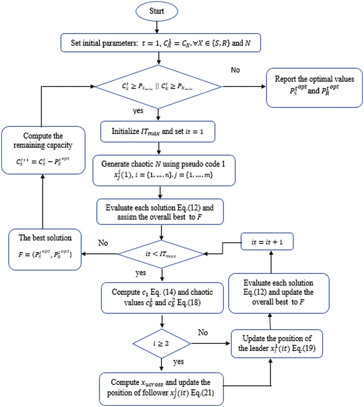
Figure 5: Flowchart of the proposed HCSSC algorithm

4  Experimental Results and Analysis

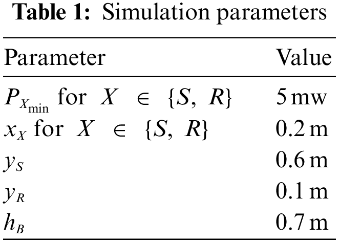
This section presents the numerical results illustrating the performance of the proposed HCSSC based power optimization scheme. Simulations are done using MATLAB-R2015a running on Windows 7 with 2 GB RAM memory. Simulation results are obtained by averaging over 1000 channel iterations. We assume that source and relay nodes have equal batteries power capacities C(i.e., C=CX) and equal maximum allowed powers PXmax=Pmax. Authors in [13] determine the mathematical computation of UG2UG and UG2AG path losses. Tab. 1 summarizes the set of the system parameters and their corresponding values.

The improvement of the resource efficiency using the proposed HCSSC algorithm, REHCSSC, against the resource efficiency, which uses the standard SSA, RESSA, is computed as follows:

impovement performance(%)=REHCSSC−RESSARESSA×100(22)

In order to demonstrate the effectiveness of chaos theory for generating the initial population, a set of experiments have been conducted with various number of individuals, as shown in Fig. 5, for the standard SSA ( i.e., with random initial salp positions) and SSA using chaotic map for initial positions generation with power capacity C=3w and maximum transmission power Pmax=50mw.

Fig. 6 illustrates the convergence of the resource efficiency RE obtained using both algorithms for different number of salp. Clearly, the generation of initial population using chaotic map has achieved better results in maximizing the resource efficiency compared to the standard SSA, during the number of iterations, due to the better exploration of the search space. The improvement is increased with the increase of N. Indeed, for N=5, the SSA with chaotic initial positions gains 4.9% better than standard SSA while at N=40, it gains 7% better.

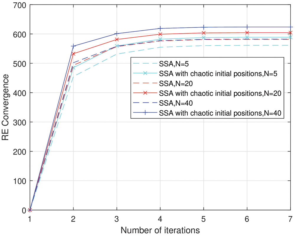
Figure 6: Convergence curves of the standard SSA and SSA using chaotic initial positions

To demonstrate the efficiency of using the chaos theory and the crossover operator to achieve a maximum resource efficiency, the proposed HCSSC algorithm has been tested for different number of salps N∈{5,10,20,40} at C=3w and Pmax=50mw, as shown in Fig. 7. The figure depicts the convergence of resource efficiency as a function of iterations numbers obtained using the proposed HCSSC algorithm in the nodes powers.

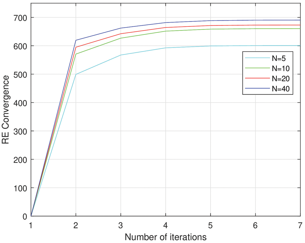
Figure 7: Convergence curve of the resource efficiency using the HCSSC algorithm

From the figure, the convergence of the proposed algorithm is rapidly obtained for various number of salps to reach the optimal RE values. Also, the increase in the number of salps enhances the computation accuracy of the optimal RE. Therefore, the proposed algorithm can be efficiently implemented with acceptable cost of computational complexity.

For a fair comparison, the individuals number involved in the swarm population and the maximum number of iterations are equal for both standard SSA and the proposed HCSSC algorithms. Tab. 2 illustrates the maximum (Max.), minimum (Min.), Average (Avg.) and Standard deviation (Std.) of RE at various N and various Pmax at C=3w. The best results are shown in bold.

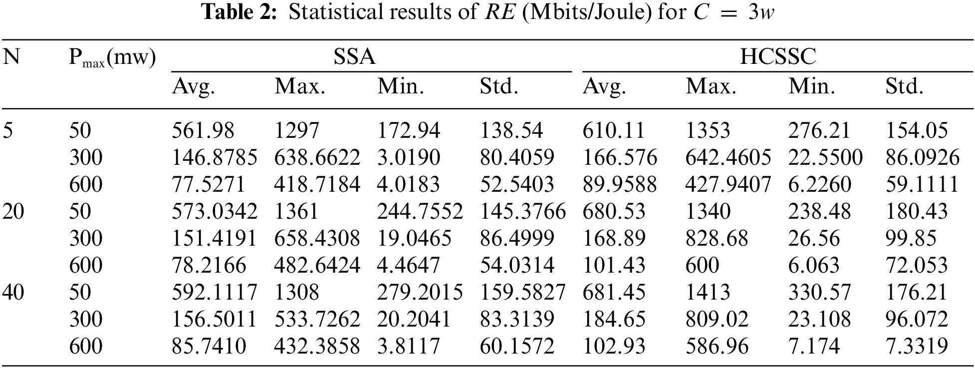
In comparison with the traditional SSA based optimization scheme, the proposed HCSSC outperforms it in all evaluated performance measurements. According to Tab. 2, for N=5 and Pmax=300mw, the average value of the RE based HCSSC reaches 166.576 (Mbits/Joule) and the average value of the RE based SSA reaches 146.8785 (Mbits/Joule). Hence, the gain is about 13%. While for N=40 and Pmax=50mw, the average value of RE based HCSSC is 681.45 (Mbits/Joule) while the average value of the RE based SSA equals 592.1117 (Mbits/Joule). So, the gain reaches 15%.

Fig. 8 shows the convergence behavior of the resource efficiency using the proposed algorithm HCSSC against the standard SSA, in nodes power optimization, with different number of salps N∈{5,20,40} at C=3w and Pmax=50mw.

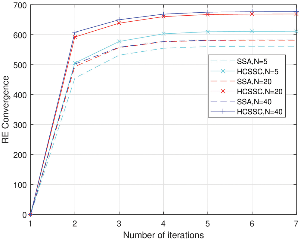
Figure 8: Convergence curve of HCSSC against standard SSA

With different number of salps, the proposed HCSSC obtains a better RE convergence than standard SSA for different number of iterations. The amelioration is raising with the increase of N. At N=5,20 and 40 the RE of HCSSC is raising up to 9%, 15% and 16%, respectively.

Furthermore, Fig. 9 illustrates the effect of the maximum power permitted for a single transmission Pmax on resource efficiency for both HCSSC and SSA with respect to different power capacity C∈{2,3,4}w and N=20.

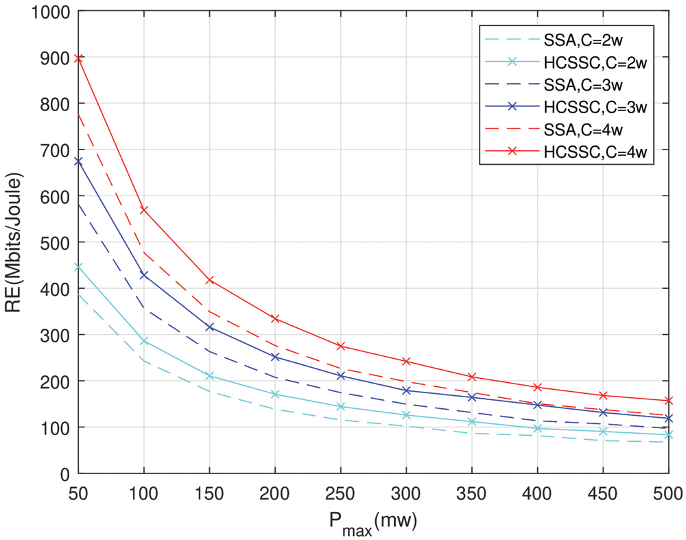
Figure 9: Resource efficiency of HCSSC and SSA vs. the maximum allowed power Pmax

Once more, compared to the power optimized SSA scheme, the HCSSC achieves a higher resource efficiency at the same power cost. Indeed, the combination of chaotic map and the cross over operations in the proposed power algorithm improves the search of optimal nodes powers considering the power physical limitations. Hence, the resource efficiency RE increases with the increase of nodes batteries capacity. Notably, the gain gap between HCSSC and SSA schemes is higher as C increases. In fact, for C=2w, the RE improvement reaches 15.3% at Pmax=50mw and reaches 19% at Pmax=400mw. While for C=4w, the gain in RE is 15.5% at Pmax=50mw and is 23.6% at Pmax=400mw.Since the increase in the maximum allowed power Pmax degrades the energy efficiency EE and the weighted spectral efficiency ωSE as well, the resource efficiency diminishes when Pmax increases. In addition, network designers can regulate Pmax depending on the accessible power resource of batteries capacities for a given resource efficiency specification.

The average consumed relay power and the average remaining relay battery per transmission for HCSSC and SSA vs.Pmax with N=20 are shown in Figs. 10 and 11, respectively. In Fig. 10, The average consumed relay power is shown for C=3w.

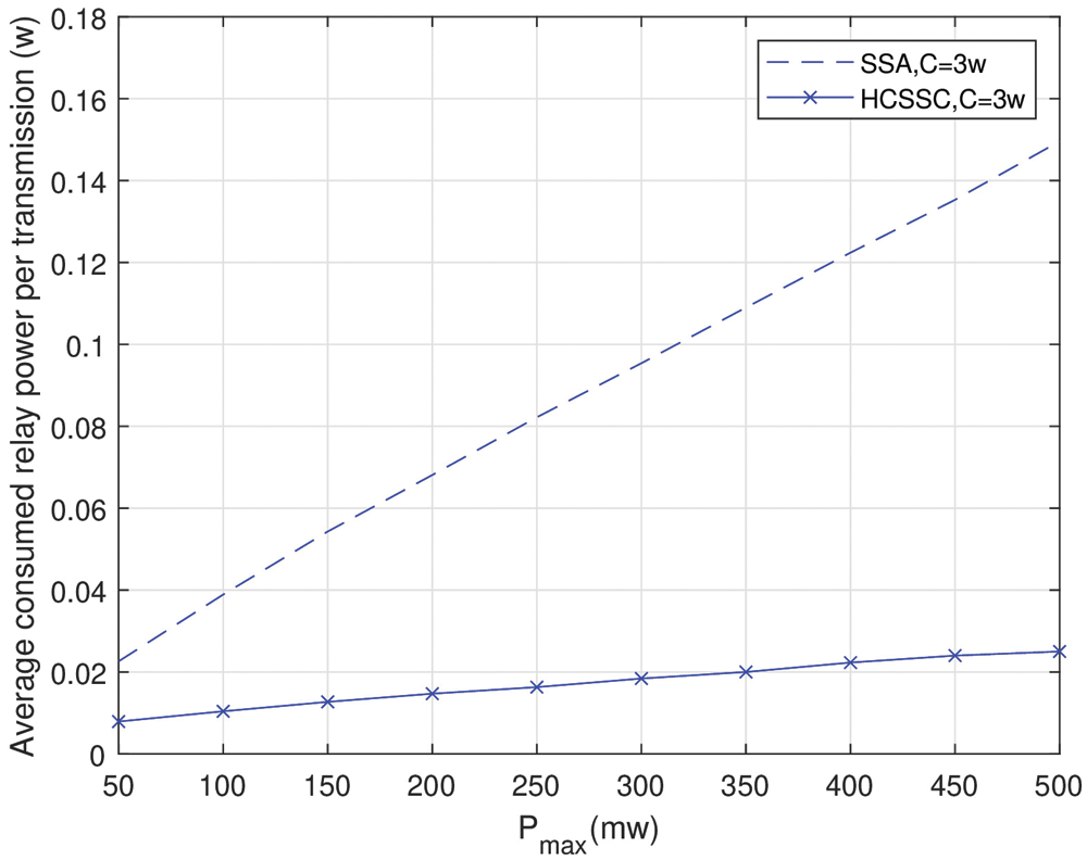
Figure 10: Average consumed relay energy per transmission (HCSSC and SSA)

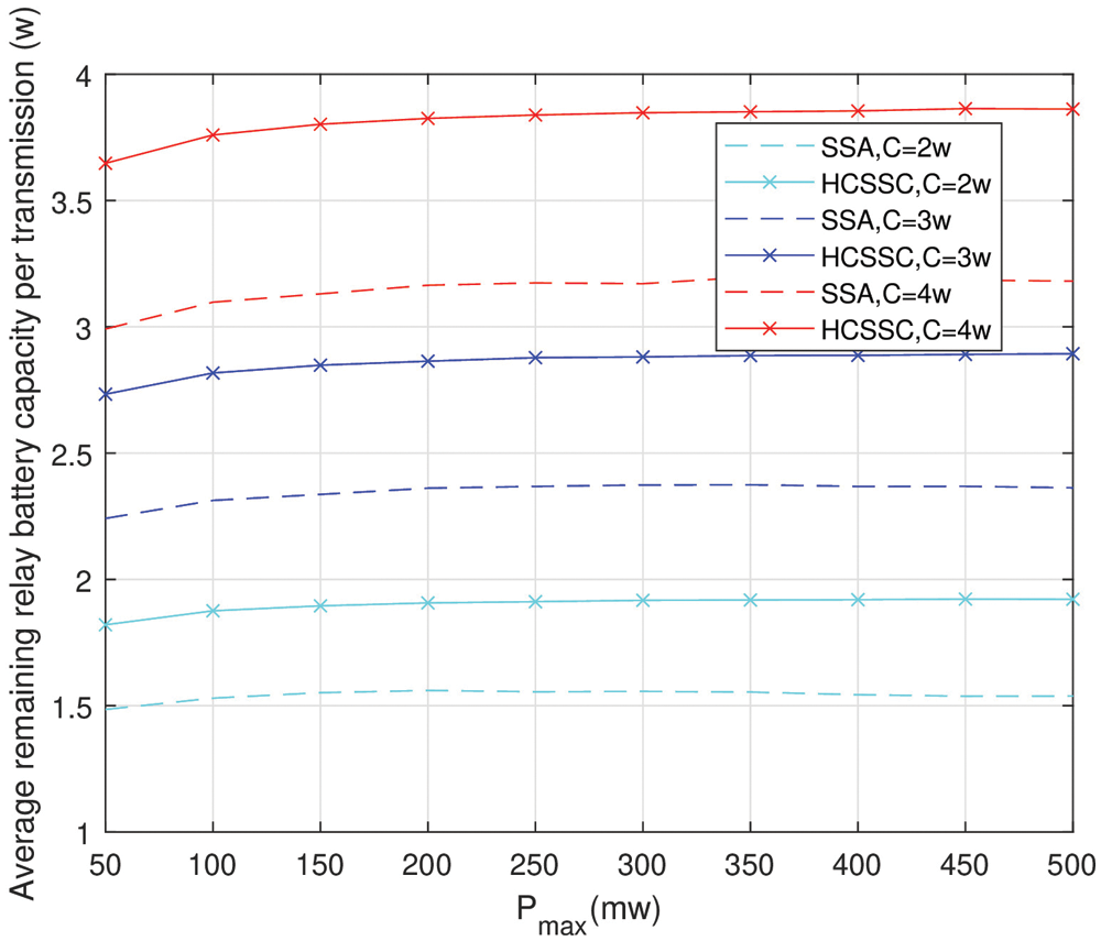
Figure 11: Average remaining relay battery per transmission (HCSSC and SSA)

Clearly, the deployment of HCSSC in nodes powers optimization allows a better relay power conservation since the average consumed relay power per transmission is minimized compared with the standard SSA along with Pmax values. In Fig. 11, the effect of the HCSSC algorithm on the average remaining relay battery per transmission compared to the SSA is illustrated for C∈{2,3,4}w. The proposed HCSSC based scheme significantly ameliorates the average remaining relay battery per transmission for all battery capacity value C. At Pmax=350mw, the obtained gain equals 23% at C=2w, it equals 21.6% at C=3w and it reaches 20.4% at C=4w. Thus, the proposed HCSSC based power optimization extends the nodes batteries lifetime and consequently the whole network lifetime.

In Fig. 12, we propose to study the resource efficiency performance in the case where the relay node has a higher battery capacity than the source node and can forward packets considering higher maximum allowed power. In fact, the relay node is expected to consume more power than the source node since it collects data from different sources to forward it to the sink node and, possibly, retransmits lost packets. Interestingly, the proposed algorithm proves its efficiency, not only in the case of equal source and relay batteries capacities, but also in the case of different source and relay batteries capacities as clearly shown in Fig. 12. We assume that PRmax=2PSmax and N=20. The proposed HCSSC based power optimization scheme achieves higher resource efficiency performance than the SSA as CS and CR increase. At CS=2w and CR=3w, the HCSSC algorithm achieves a gain of 21% better than the SSA at Psmax=50mw. While at CS=3w and CR=4w, the HCSSC algorithm achieves a gain of 28% better than the SSA at PSmax=200mw.

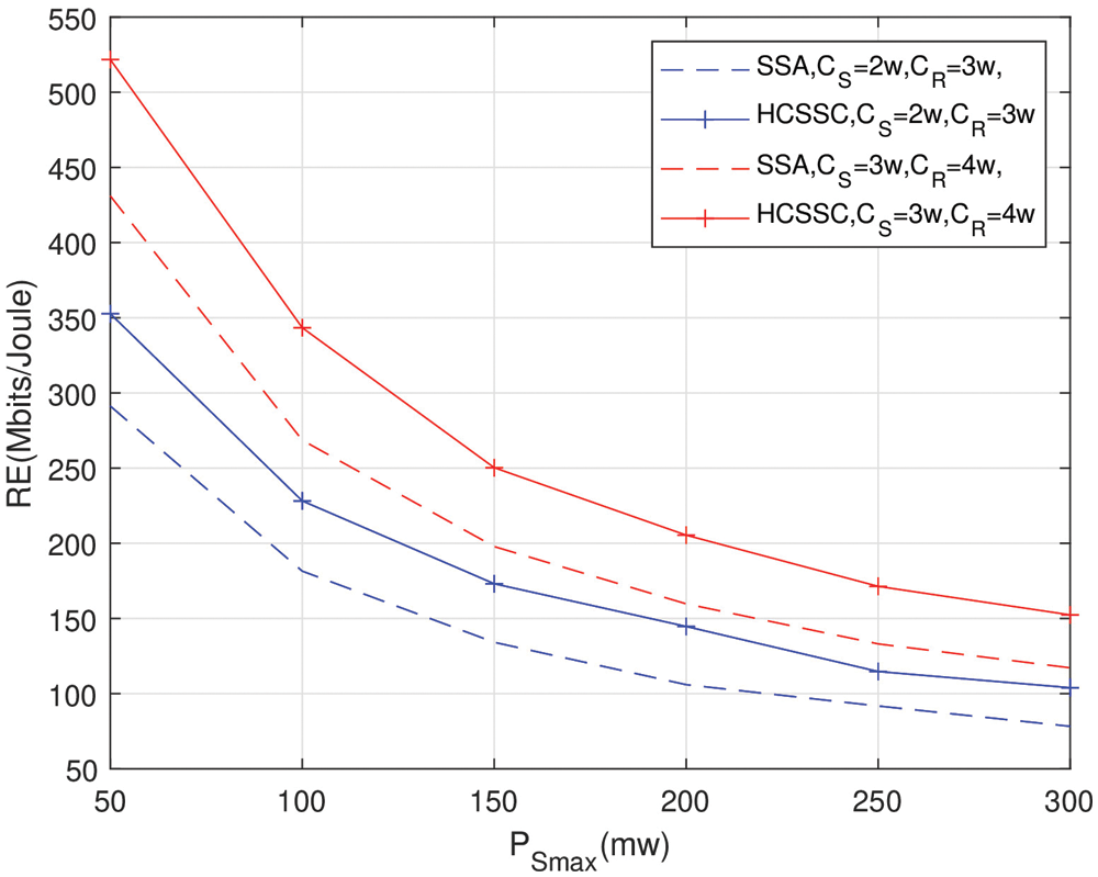
Figure 12: Resource efficiency of HCSSC and SSA for PRmax=2PSmax for different source and relay batteries capacities

In some applications, the benefit from of sensor nodes in UWSNs is restricteddue to harsh environmental conditions. For agricultural application for example, authors in [4] mention that if the water volume fraction of the mixture is high (passed 25%), the UG2UG communication link is interrupted specially with some particular soil type whose the capacity to hold the bound water is low. Consequently, the UG2UG communication can be interrupted for a long period in case of a rainfall. Also, for underground mine applications, UG2UG communications may be interrupted in many unpredictable situations such as rock falls or explosions. Moreover, we notice that the base station should implement a powerful operating system to support the additional computing complexity of the HCSSC algorithm.

5  Conclusions

This paper proposed a Hybrid Chaotic Salp Swarm with Crossover (HCSSC) algorithm for an UWSN to maximize the network resource efficiency. This last is a global metric that jointly considers the energy and the spectral efficiencies to balance the power consumption and the bandwidth usage. The algorithm improves the standard metaheuristic SSA by the use of logistic chaotic map in the generation of the initial population and the deployment of the uniform crossover operator to compute the final solution. At each packet transmission, the HCSSC is applied to provide the optimal source and relay nodes powers considering the remaining nodes batteries capacities constraints. Simulations showed that the integration of the chaotic map in the population initialization and the use of the crossover method in the positions’ updates improved the resource efficiency compared to the standard SSA for different nodes batteries capacities and different maximum allowed powers. Also, the use of the HCSSC algorithm offered a better relay power conservation proved by the minimization of the average consumed relay power per transmission and the maximization of the average remaining relay battery per transmission. Moreover, the efficiency of the proposed algorithm is demonstrated in the case where the relay node has a higher battery capacity than the source node and can forward packets considering higher maximum power. As future work, the efficiency of the proposed HCSSC algorithm in multi-relay UWSN, where many relay nodes cooperate with source nodes to transmit sensory data to the base station, will be addressed. Thus, the impact of the numbers of variables on HCSSC algorithm performance will be effectively studied. Moreover, the impact of the data packet size on the RE performance will be studied.

Funding Statement: The authors received no specific funding for this study.

Conflicts of Interest: The authors declare that they have no conflicts of interest to report regarding the present study.

This work is licensed under a Creative Commons Attribution 4.0 International License, which permits unrestricted use, distribution, and reproduction in any medium, provided the original work is properly cited.