Computers, Materials & Continua DOI:10.32604/cmc.2022.025811
Article

Bio-Inspired Numerical Analysis of COVID-19 with Fuzzy Parameters

F. M. Allehiany1, Fazal Dayan2,3,*, F. F. Al-Harbi4, Nesreen Althobaiti5, Nauman Ahmed2, Muhammad Rafiq6, Ali Raza7 and Mawahib Elamin8

1Department of Mathematical Sciences, College of Applied Sciences, Umm Al-Qura University, Makkah, 21955,Saudi Arabia
2Department of Mathematics and Statistics, University of Lahore, Lahore, Pakistan
3Department of Mathematics, School of Science, University of Management and Technology, Lahore, Pakistan
4Department of Physics, College of Science, Princess Nourah Bint Abdulrahman University, Riyadh, 11671, Saudi Arabia
5Department of Mathematics and Statistics, College of Science, Taif University, Taif, 21944, Saudi Arabia
6Department of Mathematics, Faculty of Sciences, University of Central Punjab, Lahore, Pakistan
7Department of Mathematics, Govt. Maulana Zafar Ali Khan Graduate College Wazirabad, Punjab Higher Education Department (PHED), Lahore, 54000, Pakistan
8Department of Mathematics, College of Science and Arts, Qassim University, Riyadh Al Khabra, Saudi Arabia
*Corresponding Author: Fazal Dayan. Email: fazaldayan1@gmail.com
Received: 05 December 2021; Accepted: 15 February 2022

Abstract: Fuzziness or uncertainties arise due to insufficient knowledge, experimental errors, operating conditions and parameters that provide inaccurate information. The concepts of susceptible, infectious and recovered are uncertain due to the different degrees in susceptibility, infectivity and recovery among the individuals of the population. The differences can arise, when the population groups under the consideration having distinct habits, customs and different age groups have different degrees of resistance, etc. More realistic models are needed which consider these different degrees of susceptibility infectivity and recovery of the individuals. In this paper, a Susceptible, Infected and Recovered (SIR) epidemic model with fuzzy parameters is discussed. The infection, recovery and death rates due to the disease are considered as fuzzy numbers. Fuzzy basic reproduction number and fuzzy equilibrium points have been derived for the studied model. The model is then solved numerically with three different techniques, forward Euler, Runge-Kutta fourth order method (RK-4) and the nonstandard finite difference (NSFD) methods respectively. The NSFD technique becomes more efficient and reliable among the others and preserves all the essential features of a continuous dynamical system.

Keywords: Fuzzy parameters; SIR model; NSFD scheme; fuzzy equilibrium points; fuzzy stability analysis

1  Introduction

The novel Covid-19 belongs to a large class of deadly viruses that have infected millions of people worldwide and seriously challenged not only their individual lifestyles but also the economies and GDPs of the countries themselves. Like many other research questions regarding Covid-19 disease, reliable estimation of transmission dynamics is an important part of the research. The novel Covid-19 is still a huge panic for people around the world. Various approaches are being considered to combat this deadly disease [1–12]. Noor et al. examined a Stochastic Susceptible, Exposed, Infected and Recovered (SEIR) model of the novel coronavirus by applying various computational methods such as Euler Maruyama, Euler Stochastic and Runge Kutta Stochastic to study the dynamics of the mentioned model [13]. Afzal et al. examined the clustering of Covid-19 data with the c-Means (cM) and Fuzy c-Means (Fc-M) algorithms [14]. Danane et al. examined the dynamics of a Covid-19 stochastic model with an isolation strategy and the white noise and Lévy jump disturbances are contained in all compartments of the proposed model [15]. Hussain et al. examined a stochastic model to study the transmission dynamics of Covid-19 [16]. Singh et al. proposed a fractional-order Covid-19 model based on the principle of the domain and memory discretization [17]. Baba et al. developed a mathematical model that takes into account the imposition of lockdown in Nigeria [18]. Nisar et al. developed a Susceptible, Infected, Recovered and Death (SIRD) model of Caputo's Covid-19 disease in fractional order and examined its reproduction number and stability analysis. The Adams-Bashforth fractional method is used for the model [19]. Shaikh et al. studied a Covid-19 model of bat-host-reservoir-human fractional order transmission [20]. Raza et al. presented a Susceptible, Exposed, Infected, Quarantined and Recovered (SEIQR) non-linear delayed coronavirus pandemic model and examined Routh-Hurwitz criterion, Volterra-Lyapunov function, Lasalle invariance principle and reproductive number [21]. Ghorui et al. developed a fuzzy analytical hierarchy process to determine weights and finally hesitant fuzzy sets (HFS) using a similarity-based order preference technique to determine the primary risk factor identification of Covid-19 [22]. Ahmad et al. proposed a fuzzy model with a fractional order in the sense of Caputo using the Laplace fuzzy method and the Adomian decomposition transformation [23]. Zamir et al. have developed a model that focuses on the elimination and control of Covid-19 infection [24]. Fuzzy set theory was introduced by Zadeh in 1965 [25]. Diagnosis of infectious diseases has been studied by using fuzzy theory. Barros et al. [26] proposed a new approach to integrating an ecological model with fuzzy criteria into the differential equations describing a dynamic system. Barros et al. [27] and Mondal et al. [28] have studied the epidemic models having the transmission coefficient as a fuzzy set. Verma et al. [29] have studied the fuzzy epidemic model and performed comparative studies of the equilibrium points of the disease for the classical and fuzzy models. In addition, the reproduction number of the classic and the fuzzy system were compared. The obtained analytical results were supported by some numerical simulations. Mishra et al. [30] have developed a fuzzy Susceptible–Infectious-Recovered–susceptible (SIRS) model for the transmission of worms in a computer network. The low, medium and high cases of the epidemic control of worms in the computer network were analyzed for a better understanding of the worms’ attack which may also control them. Some numerical methods were used for the solution of the developed model. Ortega et al. [31] employed the fuzzy logic for the prediction in the epidemiology related problems in the infectious disease. A model of rabies among the partially vaccinated dogs was discussed. A comparison between the fuzzy linguistic rules and classical differential equations was also done. Verma et al. [32] have studied the dynamics of Ebola virus disease by employing fuzziness in all biological parameters. Some mathematical models were prosed for the transmission trajectories of the Ebola outbreak. The existence of the equilibria and their stability were studied by employing triangular fuzzy numbers. The stability of the equilibria was related to the basic reproduction number which was calculated with the help of the next generation matrix and the numerical methods were used to support theoretical work. Das and Pal developed an SIR model with imprecise biological parameters [33]. The existence of equilibrium points and their feasibility criteria were discussed and the numerical simulation was done to support the analytical results. Sadhukhan et al. [34] studied about food chain model with optimal harvesting in a fuzzy environment. Jafelice et al. introduced a model for the evolution of the positive Human Immunodeficiency Virus (HIV) population and the manifestation of Acquired Immunodeficiency Syndrome (AIDS) [35]. Since each community changes with the evolution of the environment, even the biological parameters used in mathematical models are not always fixed [36]. The change in temperature also affects the rate of transmission of the virus in the population. Irfan et al. investigated the relationship between temperature and COVID-19 transmission in different provinces of Pakistan [37]. Low-temperature provinces were found to have strong associations between temperature and COVID-19 transmissibility. In this sense, fuzzy mathematical models are more meaningful than crisp models.

Micken's introduced the NSFD scheme [38]. Cresson et al. [39] studied the construction of the NSFD numerical scheme and discussed its different properties like convergence and stability etc. Some numerical examples were solved and a comparison with Euler, RK method of order 2 and 4 was done. Anguelov et al. [40] developed an NSFD scheme and discussed its stability analysis and dynamics preserving for a malaria model. The parameters used in existing SIR epidemic models employ crisp numbers, whereas uncertainty in parameters and heterogeneity in the population is very likely to occur. To make the model more realistic, the use of fuzzy parameters is very important. Abdy et al. presented an SIR model considering the vaccination, treatment and implementation of health protocols as fuzzy numbers and studied their effects on the spread of COVID-19 [41]. We have extended the work by presenting the comparative numerical analysis of the model using Euler, RK-4 and NSFD schemes. We started with a system of differential equations and calculated the fuzzy basic reproduction number and fuzzy equilibrium points for the proposed model. We have developed Euler, RK-4 and NSFD schemes for the studied model. Furthermore, we studied the fuzzy stability for the proposed NSFD scheme at disease-free (DF) and endemic equilibrium (EE) points respectively. Moreover, we have presented the simulation results of the developed schemes. The remaining of this article has been divided into various segments. Section 2 lays down some basic definitions related to this study. A fuzzy SIR mathematical model and its fuzziness are discussed in Section 3. The fuzzy basic reproductive number and the fuzzy equilibrium points are also computed in this section. Section 4 contains numerical modeling of the studied model. Section 5 is devoted to numerical results and discussions. This article is concluded in Section 6.

2  Preliminaries

In this section, we mention some basic definitions which will be useful for this study [42,43].

2.1 Definition 1

A fuzzy subset A of the universe set X is represented by the membership function μA(x):X→[0, 1], where μA(x) indicates the degree of membership of  x in the fuzzy set A.

2.2 Definition 2

A fuzzy subset A in R is called fuzzy number when:

•   All δ−levels of A are non-empty, with 0 ≤ δ ≤ 1, that is, A must be normal.

•   All δ−levels of A are closed intervals ofR.

•   The support of A, that is, supportA = x ∈ R: A(x) > 0 is bounded.

2.3 Definition 3

The number A=(l, m, n) is a triangular fuzzy number if its membership function is

μA(x)={0,x≤lx−lm−l,l<x≤mx−nm−n,m<x≤n0,n≤x

where  l≤m≤n.

2.4 Definition 4

A fuzzy number B = (k, l, m, n) is said to be trapezoidal if its membership function has the form of a trapezoid and is given by

μB(x)={x−kl−k,k<x≤l1,l<x≤mn−xn−m,m<x≤n0,otherwise

where  k≤l≤m≤n.

2.5 Definition 5

The expected value of a TFN A is given by

E[A]=a+2b+c4

2.6 Definition 6

The fuzzy basic reproductive number Rcf is defined as

Rcf=E[Rc(υ)]

3  SIR Epidemic Model for COVID-19 Spread with Fuzzy Parameters

In this section, we study the fuzzy basic reproduction number and the fuzzy equilibrium points respectively for the fuzzy SIR model. We considered the fuzzy SIR numerical model that has been talked about by Abdy et al.

{S′=μ−β(ζ)(1−ϱ)(1−ϖ)SI−(μ+ϱ+ϖ)SI′=β(ζ)(1−ϱ)(1−ϖ)SI−(μ+μc(ζ)+θ+γ(ζ))IR′=(θ+γ(ζ))I−(ϖ+ϱ)S−μR(1)

with S + I + R = 1. The parameters S, I and R denote proportions of susceptible, infected and recovered individuals respectively. The detail of the remaining model parameters is given in Tab. 1.

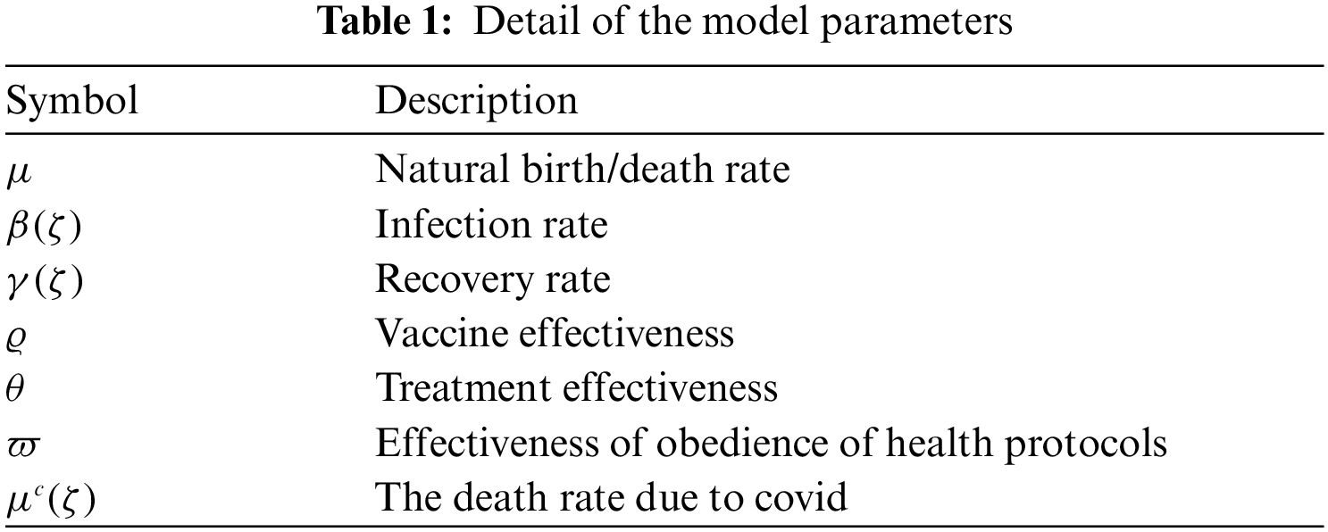
The presence or absence of the virus in epidemiology is essential to distinguish infected persons from susceptible persons. We take into account the heterogeneity of the model by considering the infection in each individual as a function of the virus-load. We assume that all infected persons do not have the same contribution to the disease transmission process and each individual has a different degree of infectivity which depends on the quantity of virus. Suppose the number of new infections is proportional to the number of encounters between infected and susceptible people, since the probability of transmission is uncertain, although it increases as infected people become more contagious. By considering the virus load of each individual, the parameters β(ζ), γ(ζ) and μc(ζ) can be displayed as a function of the coronavirus infection load ζ. The greatest chance of disease transmission is when the coronavirus infection load ζ is at its highest, the disease transmission will be negligible when the coronavirus infection load ζ is low and ζm is the minimum virus-load required for disease transmission to occur. The transmission rate is maximum at a certain point ζ0 where it is equal to (1−ϱ)(1−ϖ). The membership function of the β(ζ) is shown in Fig. 1 and it is defined as

β(ζ)={0,ζ<ζmζ−ζmζ0−ζm(1−ϱ)(1−ϖ),ζm≤ζ≤ζ01,ζ0<ζ<ζM(2)

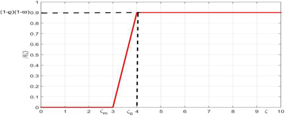
Figure 1: The membership function of β(ζ)

The recovery rate γ = γ(ζ) is also assumed to be a fuzzy number. The membership function of γ(ζ) is given by

γ(ζ)={(γ0−1)(1−θ)ζζ0,0≤ζ≤ζ0γ0(1−θ)+θ,ζ0≤ζ(3)

where the lowest recovery rate is γ0>0. The membership function of γ(ζ) is shown in Fig. 2. The higher the coronavirus infection load ζ, the more it will take to recuperate fromit.

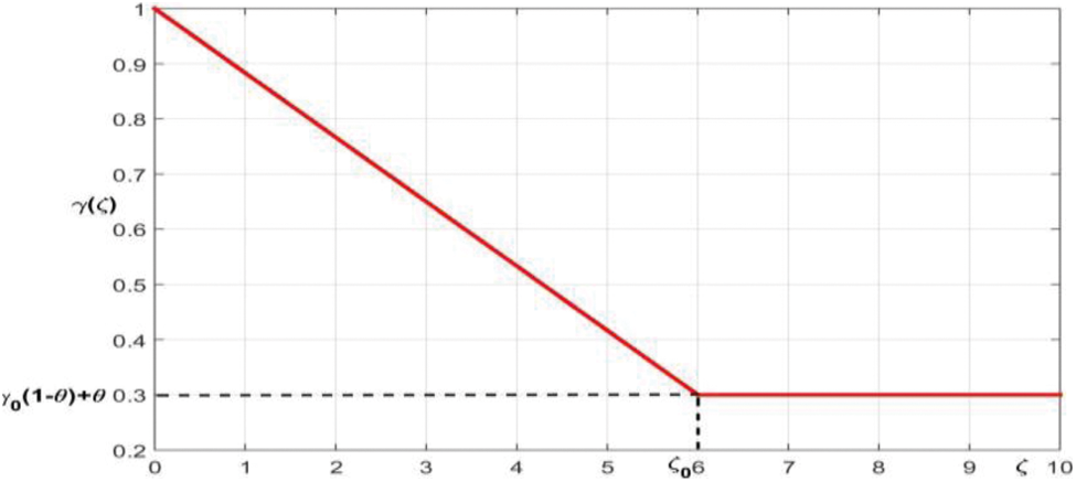
Figure 2: The membership function of γ(ζ)

The Covid-19 induced death rate μc can also be assumed as a fuzzy number and its membership function μc(ζ) is given by (depicted in Fig. 3):

μc (ζ)={(1−v−μ0c)(1−θ)ζζ0+μ0c,0≤ζ≤ζ0(1−v)(1−θ)+θμ0c,ζ0≤ζ (4)

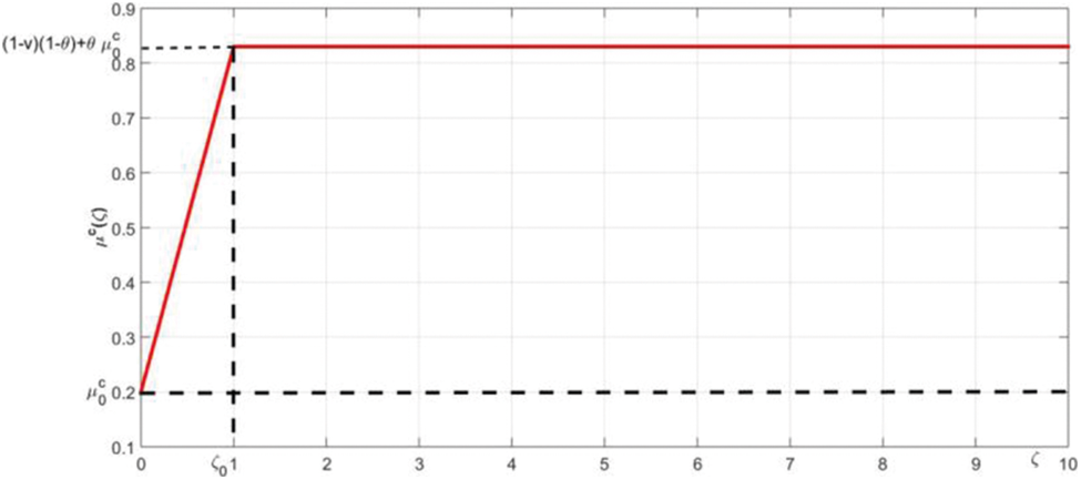
Figure 3: The membership function of μc(ζ)

The lowest death rate is μ0c(0 < μ0c < 1) and v is the effectiveness of immunity power and availability of medicine, etc. The maximum death rate is (1−v)(1−θ) + θμ0c and it may not reach the maximum value 1 due to immunity power and availability of medicine,etc.

Since the amount of virus is different for each group of individuals. To make the model more realistic, we consider only the human individuals in a given group N with classification (weak, medium and strong) given by some expert which can be seen as a linguistic variable with membership function Γ(ζ) and is given by

Γ(ζ)={0,ζ<ζ0−δδ+ζ−ζ0δ,ζ0−δ≤ζ≤ζ0δ+ζ0−ζδ,ζ0≤ζ≤ζ0+δ0,ζ>ζ0+δ(5)

3.1 Fuzzy Basic Reproduction Number

We find the value of R0 by incorporating the next generation matrix (NGM) method. Let X=[S,   I]t, then dXdt=f(x)−g(x), where

f(x)=[−β(ζ)(1−ϱ)(1−ϖ)SI−β(ζ)(1−ϱ)(1−ϖ)SI]andg(x)=[−μ+(μ+ϱ+ϖ)S(μ+μc(ζ)+θ+γ(ζ))I]

The Jacobeans of f(x) and g(x) denoted by N and M are given below.

N=[−β(ζ)(1−ϱ)(1−ϖ)I−β(ζ)(1−ϱ)(1−ϖ)Sβ(ζ)(1−ϱ)(1−ϖ)Iβ(ζ)(1−ϱ)(1−ϖ)S],and

M=[μ+ϱ+ϖ00μ+μc(ζ)+θ+γ(ζ)]

Substituting the DFE point (μμ+ϱ+ϖ,   0, ϱ+ϖμ+ϱ+ϖ) in the product NM−1 and calculating its spectral radius we get, R0(ζ)= μβ(ζ)(1−ϱ)(1−ϖ)(μ+ϱ+ϖ)(μ+μc(ζ)+θ+γ(ζ)).

Since R0(ζ) is a function of the amount of virus ζ, we analyze it for different amounts of virus.

Case 1: If ζ<ζm, β(ζ)=0, γ(ζ)>0, μc (ζ)>0, then R0(ζ)=0.

Case 2: If ζm≤ζ≤ζ0, β(ζ)=ζ−ζmζ0−ζm(1−ϱ)(1−ϖ), γ(ζ)>0 and μc (ζ)>0, then R0(ζ)= μβ(ζ)(1−ϱ)(1−ϖ)(μ+ϱ+ϖ)(μ+μc(ζ)+θ+γ(ζ)).

Case 3: If ζ0<ζ<ζM, β(ζ)=1, γ(ζ)>0 and μc (ζ)>0, then R0(ζ)= μ(ζ)(1−ϱ)(1−ϖ)(μ+ϱ+ϖ)(μ+μc(ζ)+θ+γ(ζ)).

The basic reproduction number R0(υ) is an increasing function of the parasitic virus load υ and it is well-defined as a fuzzy variable. Consequently, the expected value of R0(ζ) is well-defined and it can be expressed as a triangular fuzzy number as:

R0(ζ)=(0, μβ∗(ζ)(1−ϱ)(1−ϖ)(μ+ϱ+ϖ)(μ+μc(ζ)+θ+γ(ζ)),μ(ζ)(1−ϱ)(1−ϖ)(μ+ϱ+ϖ)(μ+μc(ζ)+θ+γ(ζ)) )

where β∗(ζ)=ζ−ζmζ0−ζm(1−ϱ)(1−ϖ).

Now we find the fuzzy basic reproduction number as follows

R0f=E[R0(ζ)]

R0f=μ(1−ϱ)(1−ϖ)4(2β(ζ)(+1(μ+ϱ+ϖ)(μ+μc(ζ)+θ+γ(ζ)))

where β∗(ζ)=ζ−ζmζ0−ζm(1−ϱ)(1−ϖ).

3.2 Fuzzy Equilibrium Points

Case 1: If ζ<ζm, then β(ζ)=0, γ(ζ)>0 and μc (ζ)>0. From system (1), we get S=μμ+ϱ+ϖ, I=0 and R=ϱ+ϖμ+ϱ+ϖ. Therefore, we obtain

C0(S0,I0,R0)=(μμ+ϱ+ϖ,   0, ϱ+ϖμ+ϱ+ϖ)

which is the disease-free equilibrium point. It is the situation when there is no virus in the population. Biologically, when the amount of virus is less than a minimum amount required in the population for disease transmission, the disease will dieout.

Case 2: If ζm≤ζ≤ζ0, then β(ζ)=ζ−ζmζ0−ζm(1−ϱ)(1−ϖ), γ(ζ)>0 and μc (ζ)>0. From system (1), we obtain,

C∗(S∗,I∗,R∗)=(μ+μc(ζ)+θ+γ(ζ)β(ζ)(1−ϱ)(1−ϖ),   μμ+μc(ζ)+θ+γ(ζ)−μ+ϱ+ϖβ(ζ)(1−ϱ)(1−ϖ),(θ+γ(ζ))I∗(ϱ+ϖ)S∗μ)

Case 3: If ζ0<ζ<ζM, then β(ζ)=1, γ(ζ)>0 and μc (ζ)>0. From system (1), we obtain

C∗∗(S∗∗,I∗∗,R∗∗)=(μ+μc(ζ)+θ+γ(ζ)(ζ)(1−ϱ)(1−ϖ),   μμ+μc(ζ)+θ+γ(ζ)−μ+ϱ+ϖ(ζ)(1−ϱ)(1−ϖ),(θ+γ(ζ))I∗∗(ϱ+ϖ)S∗∗μ)

The equilibrium points C∗( S∗,I∗,R∗) and C∗∗( S∗∗,I∗∗,R∗∗) are called endemic equilibrium points. These equilibriums occur when the virus is greater than the minimum amount required and it persists in the population.

4  Numerical Modeling

In this section, we will construct three numerical schemes, i.e., Euler, RK-4 and NSFD to solve the system of differential equations corresponding to the fuzzy SIR model. Furthermore, we will discuss the fuzzy stability of the NSFD scheme for the fuzzy SIR model at DFE point (μμ+ϱ+ϖ,   0, ϱ+ϖμ+ϱ+ϖ) and EE points C∗( S∗,I∗,R∗) and C∗∗( S∗∗,I∗∗,R∗∗) respectively.

4.1 Forward Euler Method

Forward Euler strategy is a notable time forward finite difference scheme which is expressed in nature. This finite difference method is produced for the above system as,

sn+1=sn+h[μ−β(ζ)(1−ϱ)(1−ϖ)snin−(μ+ϱ+ϖ)sn](6)

in+1=in+hin[β(ζ)(1−ϱ)(1−ϖ)sn−(μ+μc(ζ)+θ+γ(ζ))](7)

rn+1=rn+h[(θ+γ(ζ))in−(ϖ+ϱ)sn−μrn](8)

where, h is the step at anytime.

4.2 Runge-Kutta Method

RK-4 is also a notable time forward explicit finite difference scheme. To develop an explicit RK-4 method we again consider the above the above system, wehave

Step 1

k1=h[μ−β(ζ)(1−ϱ)(1−ϖ)snin−(μ+ϱ+ϖ)sn]               

m1=hin[β(ζ)(1−ϱ)(1−ϖ)sn−(μ+μc(ζ)+θ+γ(ζ))]           

n1=h[(θ+γ(ζ))in−(ϖ+ϱ)sn−μrn]     

Step 2

k2=h[μ−β(ζ)(1−ϱ)(1−ϖ)(sn+k12)(in+m12)−(μ+ϱ+ϖ)(sn+k12)]               

m2=h(in+m12)[β(ζ)(1−ϱ)(1−ϖ)(sn+k12)−(μ+μc(ζ)+θ+γ(ζ))]            

n2=h[(θ+γ(ζ))(in+m12)−(ϖ+ϱ)(sn+k12)−μ(rn+n12)]     

Step 3

k3=h[μ−β(ζ)(1−ϱ)(1−ϖ)(sn+k22)(in+m22)−(μ+ϱ+ϖ)(sn+k22)]               

m3=h(in+m22)[β(ζ)(1−ϱ)(1−ϖ)(sn+k22)−(μ+μc(ζ)+θ+γ(ζ))]            

n3=h[(θ+γ(ζ))(in+m22)−(ϖ+ϱ)(sn+k22)−μ(rn+n22)]     

Step 4

k3=h[μ−β(ζ)(1−ϱ)(1−ϖ)(sn+k3)(in+m3)−(μ+ϱ+ϖ)(sn+k3)]               

m3=h(in+m3)[β(ζ)(1−ϱ)(1−ϖ)(sn+k3)−(μ+μc(ζ)+θ+γ(ζ))]            

n3=h[(θ+γ(ζ))(in+m3)−(ϖ+ϱ)(sn+k3)−μ(rn+n3)]     

The final results of RK-4 are

sn+1=sn+16[k1+2k2+2k3+k4](9)

in+1=in+16[m1+2m2+2m3+m4](10)

rn+1=rn+16[n1+2n2+2n3+n4](11)

4.3 Non-Standard Finite Difference Method

Now we will build NSFD scheme for the fuzzy SIR model, based on Micken's theory. To develop an explicit NSFD scheme we again consider the system (1), we have

sn+1=sn+hμ1+h[μ−β(ζ)(1−ϱ)(1−ϖ)in−(μ+ϱ+ϖ)](12)

in+1=hin[β(ζ)(1−ϱ)(1−ϖ)sn+1]1+h(μ+μc(ζ)+θ+γ(ζ))(13)

rn+1=rn+h[(θ+γ(ζ))in+1+(ϖ+ϱ)sn+1]1+hμ(14)

where, h is the step at anytime.

4.4 Fuzzy Stability of the NSFD Scheme

To check the stability of the NSFD scheme of the fuzzy SIR model at DFE point (μμ+ϖ+ϱ,   0, ϖ+ϱμ+ϖ+ϱ) and EE points C∗( S∗,I∗,R∗) and C∗∗( S∗∗,I∗∗,R∗∗) respectively, let

F=s+hμ1+h[μ−β(ζ)(1−ϱ)(1−ϖ)i−(μ+ϱ+ϖ)](15)

G=hi[β(ζ)(1−ϱ)(1−ϖ)s]1+h(μ+μc(ζ)+θ+γ(ζ))(16)

H=r+h[(θ+γ(ζ))i+(ϖ+ϱ)s]1+hμ(17)

Jacobean matrix of Eqs. (14) to (16) is

J=[11+h[μ−β(ζ)(1−ϱ)(1−ϖ)i−(μ+ϱ+ϖ)]−h(s+hμ)β(ζ)(1−ϱ)(1−ϖ)[1+h[μ−β(ζ)(1−ϱ)(1−ϖ)i−(μ+ϱ+ϖ)]]20hβ(ζ)(1−ϱ)(1−ϖ)i1+h(μ+μc(ζ)+θ+γ(ζ))1+hβ(ζ)(1−ϱ)(1−ϖ)s1+h(μ+μc(ζ)+θ+γ(ζ))0h(ϱ+ϖ)1+hμh(θ+γ(ζ))1+hμ11+hμ]

Case 1: If ζ<ζm, then β(ζ)=0, γ(ζ)>0, and μc (ζ)>0.

Jacobean at the DFE point C0(S0,I0,R0)=(μμ+ϱ+ϖ,   0, ϱ+ϖμ+ϱ+ϖ) is

J0=[11+h(μ+ϱ+ϖ)00011+h(μ+μc(ζ)+θ+γ(ζ))0h(ϱ+ϖ)1+hμh(θ+γ(ζ))1+hμ11+hμ]

The above numerical scheme will be unconditionally convergent if the absolute eigenvalue of the above Jacobean matrix at the DFE point is less than unity, i.e., |λi|<1, i=1, 2, 3.  From above Jacobean matrix J0 we obtain the eigenvalues λ1=11+h\mu <1, λ2=11+h(μ+ϱ+ϖ)<1 and λ3=11+h(μ+μc(ζ)+θ+γ(ζ))<1.

Case 2: If ζm≤ζ≤ζ0, then β(ζ)=ζ−ζmζ0−ζm(1−ϱ)(1−ϖ), γ(ζ)>0 and μc (ζ)>0.

Jacobean at the point C∗(S∗,I∗,R∗) is given as

J1=[11+h[μ−β∗(ζ)(1−ϱ)(1−ϖ)i∗−(μ+ϱ+ϖ)]−h(s∗+hμ)β∗(ζ)(1−ϱ)(1−ϖ)[1+h[μ−β∗(ζ)(1−ϱ)(1−ϖ)i∗−(μ+ϱ+ϖ)]]20hβ∗(ζ)(1−ϱ)(1−ϖ)i∗1+h(μ+μc(ζ)+θ+γ(ζ))1+hβ∗(ζ)(1−ϱ)(1−ϖ)s∗1+h(μ+μc(ζ)+θ+γ(ζ))0h(ϱ+ϖ)1+hμh(θ+γ(ζ))1+hμ11+hμ]

where i∗=μμ+μc(ζ)+θ+γ(ζ)−μ+ϱ+ϖβ(ζ)(1−ϱ)(1−ϖ), s∗=μ+μc(ζ)+θ+γ(ζ)β∗(ζ)(1−ϱ)(1−ϖ) and β∗(ζ)=ζ−ζmζ0−ζm(1−ϱ)(1−ϖ).

From above Jacobean matrix we obtain the eigenvalue λ1=11+h\mu . The other eigenvalues can be obtained from the following matrix

J1∗=[11+h[μ−β∗(ζ)(1−ϱ)(1−ϖ)i∗−(μ+ϱ+ϖ)]−h(s∗+hμ)β∗(ζ)(1−ϱ)(1−ϖ)[1+h[μ−β∗(ζ)(1−ϱ)(1−ϖ)i∗−(μ+ϱ+ϖ)]]2hβ∗(ζ)(1−ϱ)(1−ϖ)i∗1+h(μ+μc(ζ)+θ+γ(ζ))1+hβ∗(ζ)(1−ϱ)(1−ϖ)s∗1+h(μ+μc(ζ)+θ+γ(ζ))]

The largest eigenvalue has been plotted by using the MATLAB database and shown in Fig. 4a.

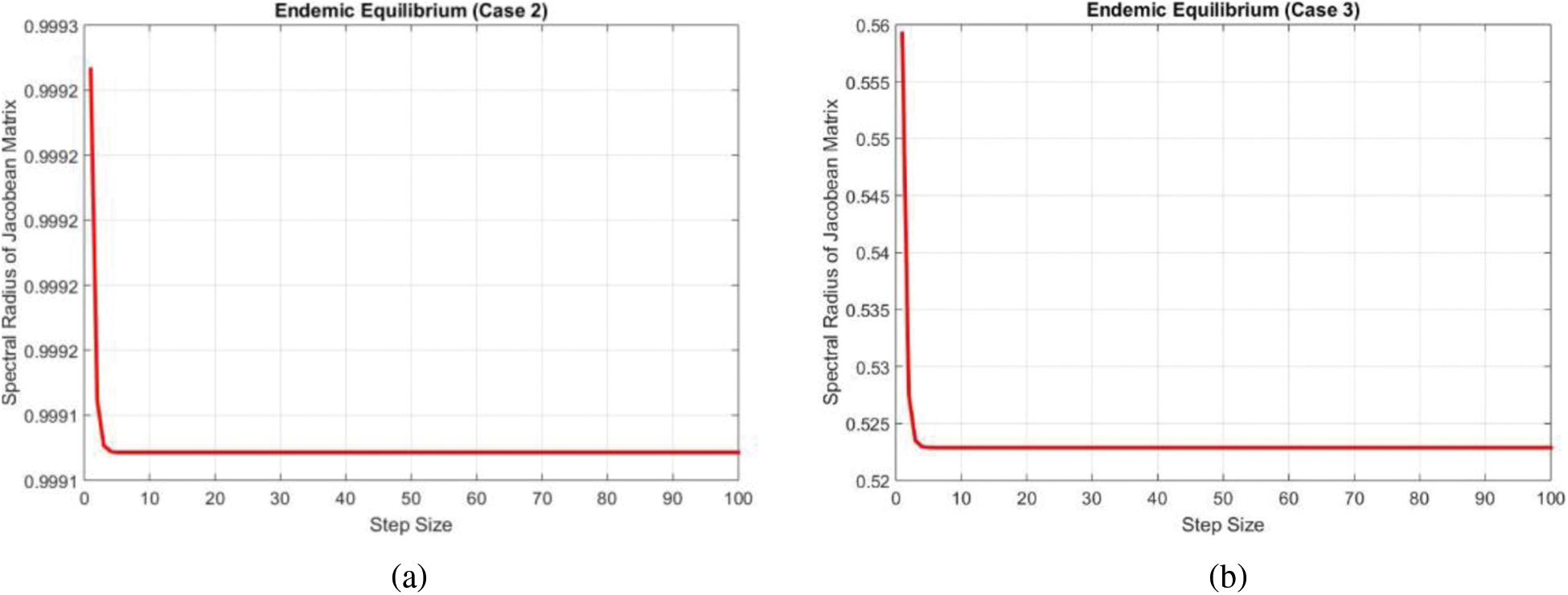
Figure 4: Eigen values of the Jacobean at the endemic equilibrium points (a) Case 2 (b) Case 3

Case 3: If ζ0<ζ<ζM, β(ζ)=1, γ(ζ)>0 and μc (ζ)>0, then R0(ζ)= μ(ζ)(1−ϱ)(1−ϖ)(μ+ϱ+ϖ)(μ+μc(ζ)+θ+γ(ζ)).

Jacobean at the point C∗∗(S∗∗,I∗∗,R∗∗) is given as

J2=[11+h[μ−(1−ϱ)(1−ϖ)i∗∗−(μ+ϱ+ϖ)]−h(s∗∗+hμ)(1−ϱ)(1−ϖ)[1+h[μ−(1−ϱ)(1−ϖ)i∗∗−(μ+ϱ+ϖ)]]20h(1−ϱ)(1−ϖ)i∗∗1+h(μ+μc(ζ)+θ+γ(ζ))1+h(1−ϱ)(1−ϖ)s∗∗1+h(μ+μc(ζ)+θ+γ(ζ))0h(ϱ+ϖ)1+hμh(θ+γ(ζ))1+hμ11+hμ]

where i∗∗=μμ+μc(ζ)+θ+γ(ζ)−μ+ϱ+ϖ(1−ϱ)(1−ϖ) and s∗∗=μ+μc(ζ)+θ+γ(ζ)(1−ϱ)(1−ϖ).

From above Jacobean matrix, we obtain the eigenvalue λ1=11+hμ. The other eigenvalues can be obtained from the following matrix

J2∗=[11+h[μ−(1−ϱ)(1−ϖ)i∗∗−(μ+ϱ+ϖ)]−h(s∗∗+hμ)(1−ϱ)(1−ϖ)[1+h[μ−(1−ϱ)(1−ϖ)i∗∗−(μ+ϱ+ϖ)]]2h(1−ϱ)(1−ϖ)i∗∗1+h(μ+μc(ζ)+θ+γ(ζ))1+h(1−ϱ)(1−ϖ)s∗∗1+h(μ+μc(ζ)+θ+γ(ζ))]

Again the largest eigenvalue has been plotted by using the MATLAB database and shown in Fig. 4b.

5  Numerical Simulation

In this segment we present the simulation results of our findings and the comparative analysis of the Euler, RK-4 and NSFD methods for the studied model.

We can examine the behavior of the fuzzy SIR epidemic model for COVID-19 spread in the above graphs. The behavior of the graphs is investigated for various values of h. Fig. 5 shows the positive behavior and convergence of Euler's method at small step sizes 0.1 and 1 respectively but diverges at step size 10. From this, we conclude that Euler's method cannot illustrate the actual behavior of the disease dynamics. In Fig. 6, the RK-4 method shows positive behavior and convergence at step sizes 0.1 and 1 but starts divergence and shows negative behavior at large step size 10. Again, we conclude that this method is also not a reliable tool for reflecting the actual behavior of the model. In Fig. 7, the NSFD method is converging to the same equilibrium points at step sizes 0.1, 1 and 10 respectively. The results show that this technique converges towards the equilibrium solution for each of the observed values of h, using step sizes 0.1, 1 and 10 with little computational effort. In this sense, this method is more robust and reliable than the standard approaches used for comparison purposes. Fig. 8, represents a comparison of Euler, RK-4 and NSFD methods at step sizes 0.1, 1 and 10 respectively. It is clear from the graphs that the NSFD method is stable, converging to equilibria and also containing positivity at all step sizes while the classical Euler and RK-4 show positivity and convergence solution at small step sizeonly.

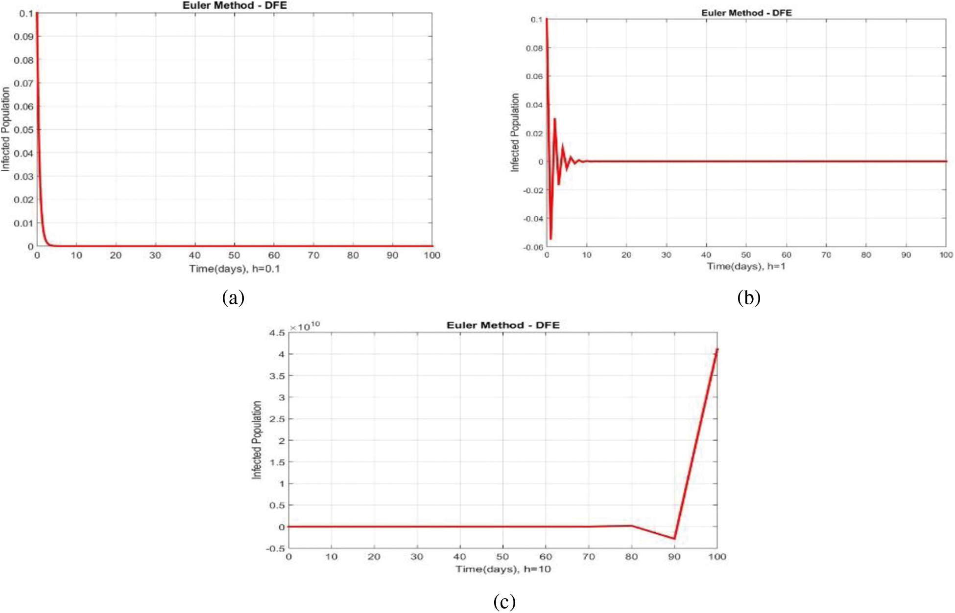
Figure 5: Portion of infected population by using Euler scheme at different step sizes (a) Infected population at h=0.1, (b) Infected population at h=1 (c) Infected population at h=10

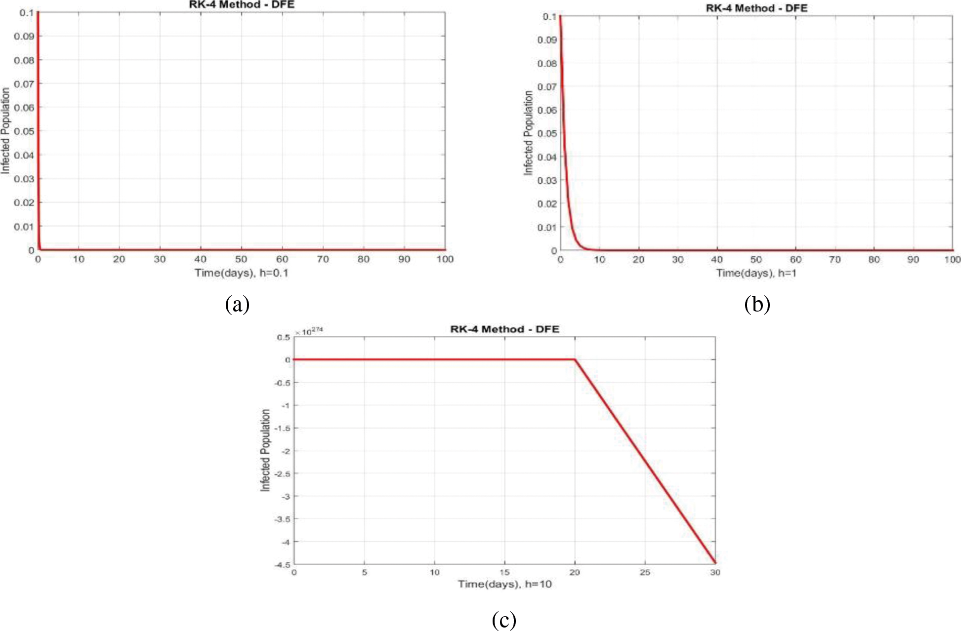
Figure 6: Portion of infected population by using RK-4 scheme at different step sizes (a) Infected population at h=0.1, (b) Infected population at h=1 (c) Infected population at h=10

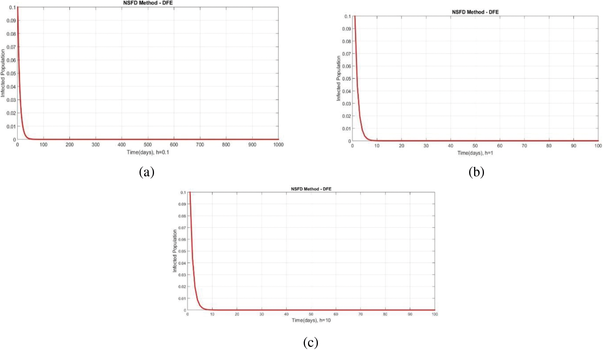
Figure 7: Portion of infected population by using NSFD scheme at different step sizes (a) Infected population at h=0.1, (b) Infected population at h=1 (c) Infected population at h=10

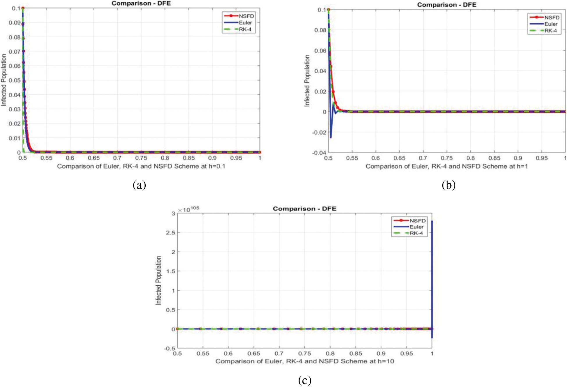
Figure 8: Comparison of Euler, RK-4 and NSFD schemes at different step sizes (a) Infected population at h=0.1, (b) Infected population at h=1 (c) Infected population at h=10

6  Conclusion

In this article, we have presented the numerical analysis of the SIR epidemic model for COVID-19 spread with fuzzy parameters. We assumed that all infected persons do not transmit the disease equally and each individual has a different degree of transfer of disease infectivity which depends on the quantity of virus. Similarly, the recovery rate and disease induced death rate are also not same for each individual. Keeping this in mind, the parameters β, γ and μc have been treated as membership functions of fuzzy numbers which depend directly on the individual's virus load. These parameters have fixed values in deterministic models and do not depend on the virus load directly. Thus the fuzzy SIR model is more realistic than the corresponding crisp model. Fuzzy equilibrium points of the studied model by considering the amounts of virus in the population have been discussed. A disease-free and two endemic equilibrium points of the fuzzy SIR model have been derived. We calculated the fuzzy basic reproduction number by utilizing next generation matrix method and the expected value of a fuzzy number. The fuzzy stability of the NSFD method has been discussed and it is shown that all of the equilibrium points have the same stability properties for the studied model. Furthermore, three numerical schemes Euler, RK-4 and NSFD are developed for our studied model. The simulation results show that the proposed NSFD technique describes the convergence solution at each time step size. While the classical Euler and RK-4 show positivity and convergence solutions at small step sizes only. The NSFD technique is an explicit numerical scheme therefore easy to implement, shows stable behavior numerically and demonstrates a good agreement with analytic results possessed by continuous model. It describes that NSFD is more reliable as compared to the other two techniques and preserves all the essential features of a continuous dynamical system. The numerical and simulations results presented in this work will provide a tribune for the researchers to compare their studies.

Acknowledgement: The authors express their gratitude to Princess Nourah bint Abdulrahman University Researchers Supporting Project (Grant No. PNURSP2022R55), Princess Nourah bint Abdulrahman University, Riyadh, Saudi Arabia.

Funding Statement: The authors received no specific funding for this study.

Conflicts of Interest: The authors declare that they have no conflicts of interest to report regarding the present study.

References

 1.  S. Ullah and M. A. Khan, “Modeling the impact of nonpharmaceutical interventions on the dynamics of novel coronavirus with optimal control analysis with a case study,” Chaos, Solitons & Fractals, vol. 139, no. 1, pp. 1–31, 2020. [Google Scholar]

 2.  M. Naveed, M. Rafiq, A. Raza, N. Ahmed, I. Khan et al., “Mathematical analysis of novel coronavirus (2019-nCov) delay pandemic model,” Computers, Materials & Continua, vol. 64, no. 3, pp. 1401–1414, 2020. [Google Scholar]

 3.  W. Shatanawi, A. Raza, M. S. Arif, K. Abodayeh, M. Rafiq et al., “An effective numerical method for the solution of a stochastic coronavirus (2019-ncovid) pandemic model,” Computers, Materials & Continua, vol. 66, no. 2, pp. 1121–1137, 2021. [Google Scholar]

 4.  N. Shahid, D. Baleanu, N. Ahmed, T. S. Shaikh, A. Raza et al., “Optimality of solution with numerical investigation for coronavirus epidemic model,” Computers, Materials & Continua, vol. 67, no. 2, pp. 1713–1728, 2021. [Google Scholar]

 5.  N. Ahmed, D. Baleanu, M. Rafiq, A. Raza, A. H. Soori et al., “Dynamical behavior and sensitivity analysis of a delayed coronavirus epidemic model,” Computers, Materials & Continua, vol. 65, no. 1, pp. 225–241, 2020. [Google Scholar]

 6.  M. A. Aba-Oud, A. Ali, H. Alrabaiah, S. Ullah, M. A. Khan et al., “A fractional order mathematical model for COVID-19 dynamics with quarantine, isolation, and environmental viral load,” Advances in Difference Equations, vol. 106, no. 1, pp. 1–19, 2021. [Google Scholar]

 7.  W. Gao, P. Veeresha, D. G. Prakasha and H. M. Baskonus, “Novel dynamic structures of 2019-nCOV with nonlocal operator via powerful computational technique,” Biology, vol. 9, no. 5, pp. 1–19, 2020. [Google Scholar]

 8.  M. A. Khan and A. Atangana, “Modeling the dynamics of novel coronavirus (2019-nCov) with fractional derivative,” Alexandria Engineering Journal, vol. 59, no. 4, pp. 2379–2389, 2020. [Google Scholar]

 9.  A. Atangana and S. IGretaraz, “A novel covid-19 model with fractional differential operators with singular and non-singular kernels: Analysis and numerical scheme based on newton polynomial,” Alexandria Engineering Journal, vol. 60, no. 4, pp. 3781–3806, 2021. [Google Scholar]

10. M. A. Khan, A. Atangana and E. A. Fatmawati, “The dynamics of COVID19 with quarantined and isolation,” Advances in Difference Equations, vol. 2020, no. 1, pp. 1–22, 2020. [Google Scholar]

11. M. A. Khan, S. Ullah and S. Kumar, “A robust study on 2019-nCOV outbreaks through non-singular derivative,” European Physical Journal Plus, vol. 136, no. 2, pp. 168–178, 2021. [Google Scholar]

12. M. Rafiq, J. Ali, M. B. Riaz and J. Awrejcewicz, “Numerical analysis of a bi-modal covid-19 SITR model,” Alexandria Engineering Journal, vol. 61, no. 1, pp. 227–235, 2022. [Google Scholar]

13. M. A. Noor, A. Raza, M. S. Arif, M. Rafiq, K. S. Nisar et al., “Non-standard computational analysis of the stochastic COVID-19 pandemic model: An application of computational biology,” Alexandria Engineering Journal, vol. 61, no. 1, pp. 619–630, 2022. [Google Scholar]

14. A. Afzal, Z. Ansari, S. Alshahrani, A. K. Raj, M. S. Kuruniyan et al., “Clustering of COVID-19 data for knowledge discovery using c-means and fuzzy c-means,” Results in Physics, vol. 29, no. 1, pp. 1–18, 2021. [Google Scholar]

15. J. Danane, K. Allali, Z. Hammouch and K. S. Nisar, “Mathematical analysis and simulation of a stochastic COVID-19 lévy jump model with isolation strategy,” Results in Physics, vol. 23, no. 1, pp. 1–19, 2021. [Google Scholar]

16. G. Hussain, T. Khan, A. Khan, M. Inc, G. Zaman et al., “Modeling the dynamics of novel coronavirus (COVID-19) via stochastic epidemic model,” Alexandria Engineering Journal, vol. 60, no. 4, pp. 4121–4130, 2021. [Google Scholar]

17. H. Singh, H. M. Srivastava, Z. Hammouch and K. S. Nisar, “Numerical simulation and stability analysis for the fractional-order dynamics of COVID-19,” Results in Physics, vol. 20, no. 1, pp. 1–20, 2021. [Google Scholar]

18. I. A. Baba, A. Yusuf, K. S. Nisar, A. H. Abdel-Aty and T. A. Nofal, “Mathematical model to assess the imposition of lockdown during COVID-19 pandemic,” Results in Physics, vol. 20, no. 1, pp. 1–18, 2021. [Google Scholar]

19. K. S. Nisar, S. Ahmad, A. Ullah, K. Shah, H. Alrabaiah et al., “Mathematical analysis of SIRD model of COVID-19 with caputo fractional derivative based on real data,” Results in Physics, vol. 21, no. 1, pp. 1–9, 2021. [Google Scholar]

20. A. S. Shaikh, I. N. Shaikh and K. S. Nisar, “A mathematical model of COVID-19 using fractional derivative: Outbreak in India with dynamics of transmission and control,” Advances in Difference Equations, vol. 20, no. 1, pp. 1–19, 2020. [Google Scholar]

21. A. Raza, A. Ahmadian, M. Rafiq, S. Salahshour and M. Ferrara, “An analysis of a nonlinear susceptible-exposed-infected-quarantine-recovered pandemic model of a novel coronavirus with delay effect,” Results in Physics, vol. 21, no. 1, pp. 1–18, 2021. [Google Scholar]

22. N. Ghorui, A. Ghosh, S. P. Mondal, M. Y. Bajuri, A. Ahmadian et al., “Identification of dominant risk factor involved in spread of COVID-19 using hesitant fuzzy MCDM methodology,” Results in Physics, vol. 21, no. 1, pp. 1–18, 2021. [Google Scholar]

23. S. Ahmad, A. Ullah, K. Shah, S. Salahshour, A. Ahmadian et al., “Fuzzy fractional-order model of the novel coronavirus,” Advances in Difference Equations, vol. 2020, no. 1, pp. 1–17, 2020. [Google Scholar]

24. M. Zamir, K. Shah, F. Nadeem, M. Y. Bajuri, A. Ahmadian et al., “Threshold conditions for global stability of disease-free state of COVID-19,” Results in Physics, vol. 21, no. 1, pp. 1–18, 2021. [Google Scholar]

25. L. A. Zadeh, “Fuzzy sets,” Information Control, vol. 8, no. 1, pp. 338–353, 1965. [Google Scholar]

26. L. C. Barros and R. C. Bassanezi, “A simple model of life expectancy with subjective parameters,” Kybernets, vol. 24, no. 7, pp. 57–62, 1995. [Google Scholar]

27. L. C. Barros, M. B. F. Leite and R. C. Bassanezi, “The SI epidemiological models with a fuzzy transmission parameter,” Computers & Mathematics with Applications, vol. 45, no. 10, pp. 1619–1628, 2003. [Google Scholar]

28. P. K. Mondal, S. Jana, P. Haldar and T. K. Kar, “Dynamical behavior of an epidemic model in a fuzzy transmission,” International Journal of Uncertainty, Fuzziness and Knowledge-Based Systems, vol. 23, no. 5, pp. 651–665, 2015. [Google Scholar]

29. R. Verma, S. P. Tiwari and R. K. Upadhyay, “Fuzzy modeling for the spread of influenza virus and its possible control,” Computational Ecology and Software, vol. 8, no. 1, pp. 32–45, 2018. [Google Scholar]

30. B. K. Mishra and S. K. Pandey, “Fuzzy epidemic model for the transmission of worms in computer network,” Nonlinear Analysis: Real World Applications, vol. 11, no. 5, pp. 4335–4341, 2010. [Google Scholar]

31. N. R. S. Ortega, P. C. Sallum and E. Massad, “Fuzzy dynamical systems in epidemic modeling,” Kybernetes, vol. 29, no. 2, pp. 201–218, 2000. [Google Scholar]

32. R. Verma, S. P. Tiwari and R. K. Upadhyay, “Transmission dynamics of epidemic spread and outbreak of ebola in West Africa: Fuzzy modeling and simulation,” Journal of Applied Mathematics and Computing, vol. 60, no. 1, pp. 637–671, 2019. [Google Scholar]

33. A. Das and M. Pal, “A mathematical study of an imprecise SIR epidemic model with treatment control,” Journal of Applied Mathematics and Computing, vol. 56, no. 1, pp. 477–500, 2018. [Google Scholar]

34. D. Sadhukhan, L. N. Sahoo, B. Mondal and M. Maitri, “Food chain model with optimal harvesting in fuzzy environment,” Journal of Applied Mathematics and Computing, vol. 34, no. 1, pp. 1–18, 2010. [Google Scholar]

35. R. Jafelice, L. C. Barros, R. C. Bassanezei and F. Gomide, “Fuzzy modeling in symptomatic HIV virus infected population,” Bulletin of Mathematical Biology, vol. 66, no. 6, pp. 1597–1620, 2004. [Google Scholar]

36. P. Panja, S. K. Mondal and J. Chattopadhyay, “Dynamical study in fuzzy threshold dynamics of a cholera epidemic model,” Fuzzy Information and Engineering, vol. 9, no. 3, pp. 381–401, 2017. [Google Scholar]

37. M. Irfan, M. Ikram, M. Ahmad, H. Wu and Y. Hao, “Does temperature matter for COVID-19 transmissibility? Evidence across Pakistani provinces,” Environmental Science and Pollution Research, vol. 28, no. 2, pp. 59705–59719, 2021. [Google Scholar]

38. R. E. Mickens, “A fundamental principle for constructing non-standard finite difference schemes for differential equations,” Journal of Difference Equations and Applications, vol. 11, no. 2, pp. 645–653, 2005. [Google Scholar]

39. J. Cresson and F. Pierret, “Nonstandard finite difference schemes preserving dynamical properties,” Journal of Computational and Applied Mathematics, vol. 303, no. 2, pp. 15–30, 2016. [Google Scholar]

40. R. Anguelov, Y. Dumont, J. Lubuma and E. Mureithi, “Stability analysis and dynamics preserving nonstandard finite difference schemes for a malaria model,” Mathematical Population Studies, vol. 20, no. 2, pp. 101–122, 2013. [Google Scholar]

41. M. Abdy, S. Side, S. Annas, W. Nur and W. Sanusi, “An SIR epidemic model for COVID-19 spread with fuzzy parameter: The case of Indonesia,” Advances in Difference Equations, vol. 21, no. 1, pp. 1–17, 2021. [Google Scholar]

42. Y. T. Mangongo, J. D. K. Bukweli and J. D. B. Kampempe, “Fuzzy global stability analysis of the dynamics of malaria with fuzzy transmission and recovery rates,” American Journal of Operations Research, vol. 11, no. 6, pp. 257–282, 2021. [Google Scholar]

43. L. C. Barros, R. C. Bassanezi and W. A. Lodwick, “The extension principle of zadeh and fuzzy numbers,” in A First Course in Fuzzy Logic, Fuzzy Dynamical Systems, and Biomathematics, Berlin, Germany: Springer International Publishing, pp. 23–41, 2017. [Online]. Available: https://doi.org/10.1007/978-3-662-53324-6_2. [Google Scholar]

This work is licensed under a Creative Commons Attribution 4.0 International License, which permits unrestricted use, distribution, and reproduction in any medium, provided the original work is properly cited.