Computers, Materials & Continua DOI:10.32604/cmc.2022.026225
Article

Deep Learning Framework for Precipitation Prediction Using Cloud Images

Mirza Adnan Baig*, Ghulam Ali Mallah and Noor Ahmed Shaikh

Shah Abdul Latif University, Khairpur, 77150, Pakistan
*Corresponding Author: Mirza Adnan Baig. Email: adnanbaig.iub@gmail.com
Received: 19 December 2021; Accepted: 16 February 2022

Abstract: Precipitation prediction (PP) have become one of the significant research areas of deep learning (DL) and machine vision (MV) techniques are frequently used to predict the weather variables (WV). Since the climate change has left significant impact upon weather variables (WV) and continuously changes are observed in temperature, humidity, cloud patterns and other factors. Although cloud images contain sufficient information to predict the precipitation pattern but due to changes in climate, the complex cloud patterns and rapid shape changing behavior of clouds are difficult to consider for rainfall prediction. Prediction of rainfall would provide more meticulous assistance to the farmers to know about the weather conditions and to care their cash crops. This research proposes a framework to classify the dark cloud patterns (DCP) for prediction of precipitation. The framework consists upon three steps to classify the cloud images, first step tackles noise reduction operations, feature selection and preparation of datasets. Second step construct the decision model by using convolutional neural network (CNN) and third step presents the performance visualization by using confusion matrix, precision, recall and accuracy measures. This research contributes (1) real-world clouds datasets (2) method to prepare datasets (3) highest classification accuracy to predict estimated as 96.90%.

Keywords: Machine vision; SIFT features; dark cloud patterns; precipitation; agriculture

1  Introduction

Due to the climate change classification of dark cloud patterns (DCP) and precipitation prediction (PP) are considered one of significant research areas of deep learning. Machine vision (MV) techniques are widely used to explore the hindsight knowledge of the DCP and to present the unseen insight knowledge of weather conditions [1–4]. Although cloud images contain sufficient information to predict the precipitation but due to changes in climate, the complex cloud patterns and rapid shape changing behavior of clouds are difficult to consider for rainfall prediction. Since the farmers are facing lots of difficulties to irrigate and pesticide their crops because raise in temperature and variation in precipitation patterns are dominant disturbing factors during the cultivation process [5–7]. The farmers use to observe DCP and estimates about precipitation because timely information of rainfall would provide more assistance in decision making to irrigate or pesticide their cash crops [8]. Traditionally, weather stations are being used to forecast the weather conditions around the globe and precipitation prediction is made by using online satellite cloud image analysis systems but due to the change in DCP, rainfall may not be recorded at particular coordinate of earth surface therefore machine learning framework is direly needed to construct a cloud classification model and to predict the precipitation patterns from local sky cloud images [9,10]. Cloud images reveals significant key points in shape of water vapors, cloud droplets and evaporation process which defines the capability of cloud for precipitation [11–13]; therefore we obtained key points by using scale-invariant feature transform SIFT features from cloud images and converted key points regions into tensor flow data to train and test the deep learning algorithm such as convolutional neural network. The SIFT algorithm is used to detect the sub-objects from images of clouds because it describes local features (LF) [14]. Scale-invariant feature transform extracts key points (KP) of objects from the images to formulate the reference model and prepare repository of key points (KP) [15]. We used SIFT framework to recognizes features of new image by estimating a comparison of features existing in historical data repository where feature vectors uses Euclidean distance (ED) to match object sets [15]. The algorithm determines object features and its associated variables with best match strategy such as object locations, coordinates and etc. generalized Hough transformation (GHT) and hash table (HT) are used to perform rapid estimation of object identification (OI) [16]. Several number of clusters are partitioned and at least three or more features of image meet the criteria of the subject of object than rest of features are considered as outlier and discarded accordingly. Object's KP could be extracted by supplying parameters of feature description (FD) for any given image where FDs are derived from the training images and FDs provide assistance to identify significant sub-objects from the set of multiple objects within any image. The scale, noise and illumination constructs KP where high contrast regions (HCR) pertaining to any image could represent the object and its edges for pattern recognition. In SIFT characteristics of features along with associated positions for any image may remain unchanged therefore there are fair chances for higher estimation to recognize the patterns of various objects [18]. In literature some of the nice approaches [17–24] are seen to construct the classification model but we obtained higher classification accuracy by performing a systematic approach to obtain key patterns (KP) of DCP; therefore, this paper offers a framework to classify the complex cloud patterns. The framework consists upon the three steps. In first step we preprocess the image which is also consisting upon several sub steps, in second step we construct the decision model by using convolutional neural network (CNN) and finally performance visualization by using confusion matrix, accuracy, precision and recall measures. This research contributes (1) real-world clouds datasets (2) method to prepare datasets (3) highest classification accuracy to predict PP problem estimated as 96.90%.

This paper is organized into several sections where section one presents introduction and section two describes literature review of related approaches; meanwhile section three defines the proposed methodology and section four describes the results of our proposed framework. Section five is dedicated to present the conclusion of this paper.

2  Literature Review

The approach of this paper falls into the domain of productive mining and deals with the classification problem of precipitation prediction by using dark cloud patterns. The approach proposes a data preparation method by extracting key points by using SIFT features and uses convolutional neural network (CNN) to predict the precipitation and non-precipitation conditions. Some related works are presented below.

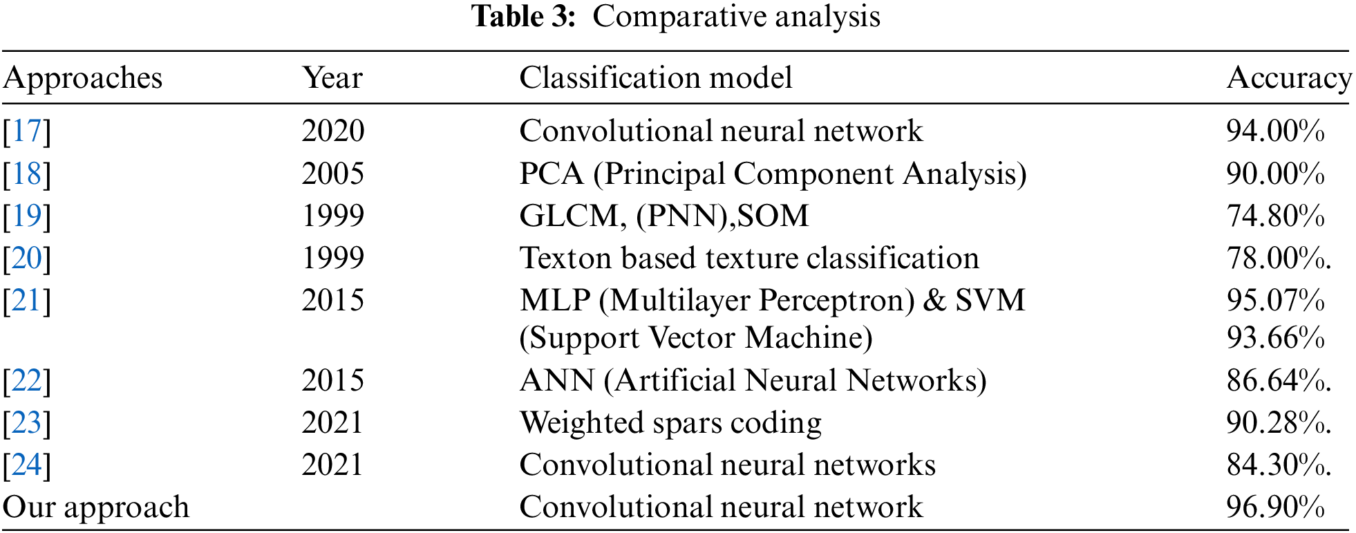
A system [17] for classification of meteorological images was proposed to classify the cloud images. The machine learning technique convolutional neural network was used with combination of an improved FDM (Frame Difference Method). Clouds such as cumulus, cirrus and stratus features were extracted by using FDM. As per shown classification accuracy, there was 94% classification accuracy to predict the cumulus, cirrus and stratus class label attributes, whereas our proposed framework contributes a data preparation technique by using the SIFT features and classification accuracy with deep learning is measured as 96.90%.

A system [18] for classification of clouds was proposed and grey scale features were used and image analysis was done with PCA (Principal Component Analysis). Clear sky, mid-level clouds and high level clouds under the classification of cumulus, cirrus and stratus class label attributes were designed and estimated 90% classification accuracy was recorded, whereas the cloud sub-images selection algorithm would more accuracy to identify the region of interest (ROI) and classification accuracy could be increased.

A comparison [19] was proposed for classification of cloud data. The GLCM (gray-level co-occurrence matrix) and artificial neural networks based algorithms such as probability neural network (PNN) and unsupervised Kohonen self-organized feature map (SOM) were used. The best classification accuracy was measured as 74.8% with SOM was estimated, whereas the key points extracted as region of interest (ROI) with descriptive quantities in SIFT features could be more reliable to detect the sub-objects from cloud images.

A cloud image classification [20] was proposed by using texture features. Texton based texture classification method and classification accuracy was measured as 78%, whereas in deep learning rest of image vectors are loaded as trainable objects which consumes a very high amount of memory however sub-images of cloud image would reduce the training and testing time and classification accuracy of our framework was measured as 96.90%.

A system [21] for classification of cloud images was proposed and MLP (Multilayer Perceptron) & SVM (Support Vector Machine) were used to build the classification model. Estimated accuracy was measured as 95.07% and 93.66% were recorded respectively, whereas we use convolutional neural network (CNN) to build the classification model and accuracy of our framework was measured as 96.90%.

A system [22] was proposed to classify the cloud images Clouds such as cumulus, cirrus. The ANN (artificial neural networks) machine learning technique was used to build the classification model. The overall classification accuracy was reported as 86.64%. Whereas accuracy of our framework was measured as 96.90%.

A compression of deep learning techniques [23] for cloud classification were proposed where deep learning machine learning technique was used and representation of weighted spars coding are used. Cloud occlusion strategy consists up several occlusions where RIWSRC estimated with highest accuracy such as 90.28%, whereas data cleaning is an important part of data preparation because real world data needs to be cleaned with appropriate methods. The accuracy of our framework was measured as 96.90%.

A system [24] for cloud classification was proposed by using convolutional neural networks. The classification accuracy was measured as 84.30%, whereas accuracy of our framework was measured as 96.90%. Prediction of precipitation would provide more meticulous assistance to farmers and complex, heterogeneous cloud patterns could efficiently be classified by using convolutional neural network (CNN).

3  Methodology

This paper proposes a framework to predict the precipitation and non-precipitation clouds and contributes (1) real-world clouds datasets (2) method to prepare datasets (3) highest classification accuracy for participation prediction (PP) problem. The proposed approach falls into the productive domain of machine vision. We use SIFT based features to find the key points based sub-images and convert them into tensor flow data. We use convolutional neural network to construct the decision model. Precision, recall, confusion matrix are used for estimating the performance evaluation of proposed approach as shown in Fig. 1. The proposed framework only deals with the clouds images.

a. Dataset

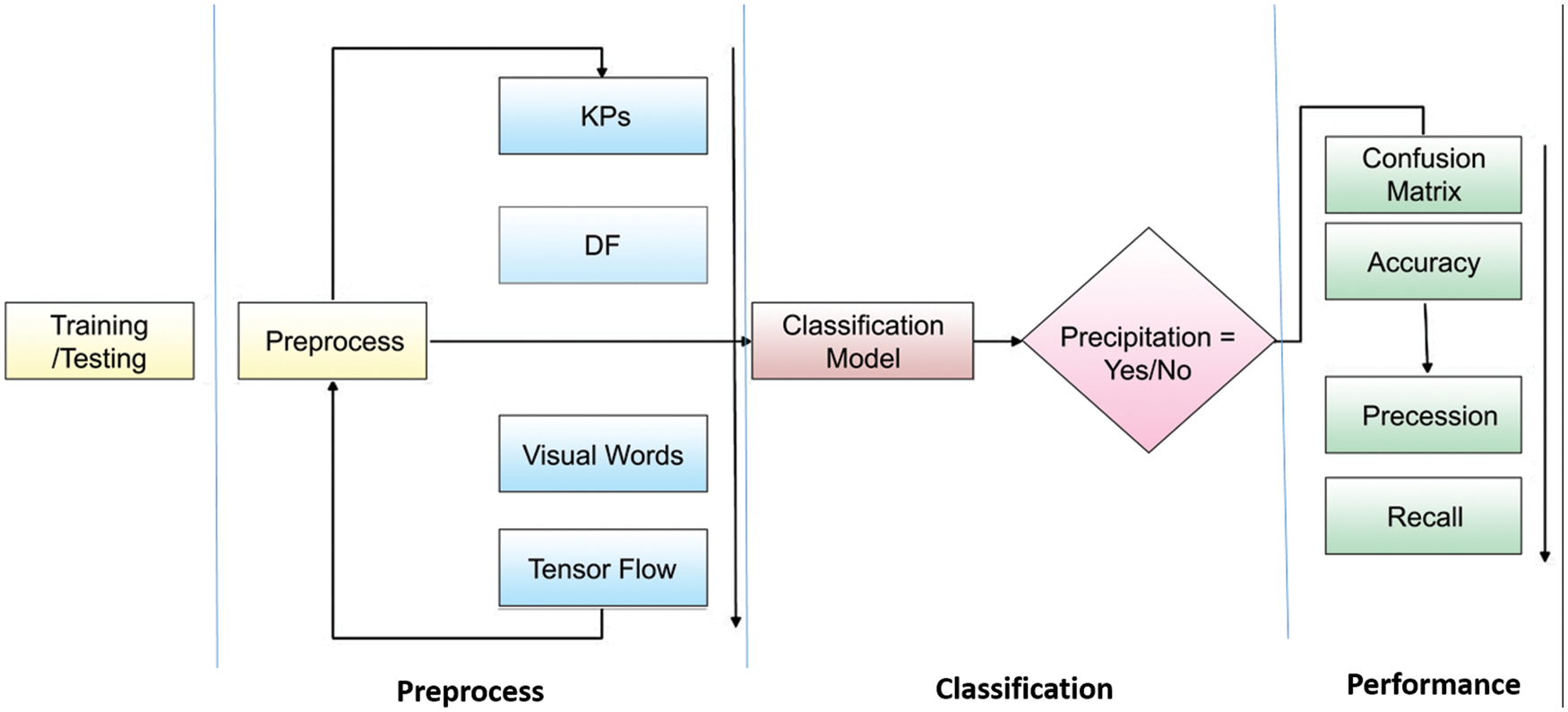
Figure 1: Deep learning framework for precipitation prediction using cloud images architecture

Cloud images captured from earth surface may become useful source for prediction the precipitation behaviors because dark cloud patterns (DCP) with variant grey appearance (VGA) are very hard to detect and classify. The videos of local precipitation patterns were downloaded from social medical applications such as Facebook. As use case we selected 10 videos for extracting the images from the frame sequences of video data. Around 400 dark cloud patterns (DCP) were selected for training and testing purposes. As per estimation each extracted image of cloud comprises over ×100 magnification power whereas the size of each image was approximated with 4000 × 2500.

b. Key Points (KPs) and Feature Description (FD)

Let's consider feature matching (FM) and feature indexing (FI) are descriptive vector data for recognizing the dark cloud patterns (DCP), where FI comprises over the functions of SIFT keys which has to identify the matching keys from the new image inputs. This feature selection technique is inspired from the experiment as conducted by Lowe in which he optimized the k-d tree algorithm, so called best-bin-first (BBF) search method. The method searches FM and FI from the images by estimating the nearest neighborhood set of pixels with highest probabilities under the limited computational time. The BBF algorithm keep the quantities of features in bins and feature space finds closest path distance to search the required patterns. KP with minimum KPs are search by mapping the minimal Euclidean distances from the descriptive vectors (DV) [25].

Therefore we transform the features by using Hugh transformation (HT) which is one of reliable method and can be used for classification of clusters by defining KPs. HT approximates clusters on the basis of ICM where analyzation of each feature can be interpreted by us FD vote strategy under higher probabilities. HT builds a hash table to match the various parameter of FD such as orientation, location and scaling where HT creates minimum 03 entries into the bin and finally bins size are sorted and decreased with respect to order orientations [26]. Every image consists upon the SIFT KPs where a 2D locations interprets coordinates of particular pixel and second property describes the ICM i.e., scale and orientation of pixel sets meanwhile the SIFT function matches all properties to vote particular object identification as per PKs training model.

Let's consider coordinates of image represented by u x v where each KPs are placed in m1,m2,  …mn meanwhile the tx and ty represents the outputs of FDs. All k-clusters could be identified by matching the parameters of (x  y)T of KPs compared with quantities of (u  v)T to perform the affine transformation [27].

[uv]=[m1m3m2m4][xy]+[txty](1)

The constructed model (tx  ty)T represents the transformation for the affine functions such as rotation, scale and stretch functions where m1 to m4 vector spaces keeps the parameters as shown in Eqs. (1) and (2).

[xy001000xy0100xy01….….….….….….….….….…][m1m2m3m4txty]=[uv..](2)

At least three matching bins are to be voted to qualify where A  x^≈b   are directly associated with matrix represented as A vectors of u and v. however let's assume AT  Ax^=ATb are the values where T could be divisible on bins as assigned to b. KPs and DF could be summarized by (AT  A)−1AT and final output of SIFT is obtained by function as per Eq. (3).

x^=(ATA)−1ATb(3)

Error detection can be done by removing the outliers where each image passes the parameters for feature model. In HT all the quantities are kept in bins which qualifies at least half of the value as per approximation [28]. Let's consider SIFT framework that creates KPs to detect the objects by convolving Gaussian filters at various scales and followed by the KPs are pointed with maximum and minim quantities of difference of Gaussian (DoG) at various scales as shown in Eq. (4) [29]. DoG image could be represented as D  (x,  y,  σ)

where image D has x,  y location summarized as G  (x,  y,  kσ) aid ∂ is the average of ICM at every pixel as shown as Fig. 2.

D(x,y,σ)=L(x,y,kjσ)−L(x,y,kjσ)(4)

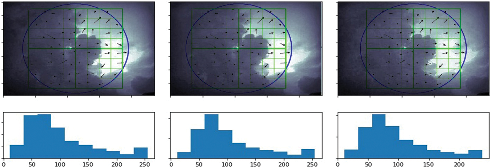
Figure 2: Finding the Feature Matching (FM) and Feature Indexing (FI) vectors from cloud images

ICM at each pixels coordinates I  (x,y) can be computed by model L  (x,  y,  kσ) contains the convolutions of the DoG original image whereas L  (x,  y,  kj  σ) is function to represent the Gaussian blur image approximated at various scales as shown in Eq. (5) [30].

L(x,y,kσ)=G(x,y,kσ)∗L(x,y)(5)

All the averages of kiσ and kjσ are loaded into the DF space where bins of G  (x,  y,  kσ)∗L  (x,  y) function recorded as cortisone product of vector spaces and pixels are weighted by assigning the aggregated quantities as ICM variables. As per interpolation theorem nearby pixels are to be matched with KPs as FD to traverse the accurately most probable locations. First KPs are determined by estimating positions and scale of candidates KPs. Let us consider the function D  (x,  y,  σ) with KPs can be expressed as per Eq. (6).

D(x)=D+∂DT∂xx+12xT∂2D∂x2x(6)

Let's consider a derivative dataset D x=  (x,y,  ∂)T consists upon KPs where strong candidates (SC) are to be selected and weak candidates (WC) are to be deleted. The matching function has to determine the coordinates x^ strong KPs by initializing x vectors from zero points. If the compared KPs and DFs are matched with user fixed parameter 0.5 threshold with available dimensions the observation will be considered as selected as shown as Fig. 3. The DFs designated as D  (x) by taking first derivative of each pixel represented as x^, where foreground information could be computed for each object, however in SIFT we can discord the object information who does not qualify 0.03 threshold value of pixel contrast otherwise the detected object's information has to be palace scale space coordinated represented by y+  x^ where y could be considered information of coordinates.

c. Visual Words (VW)

H=[DxxDxyDxyDyy](7)

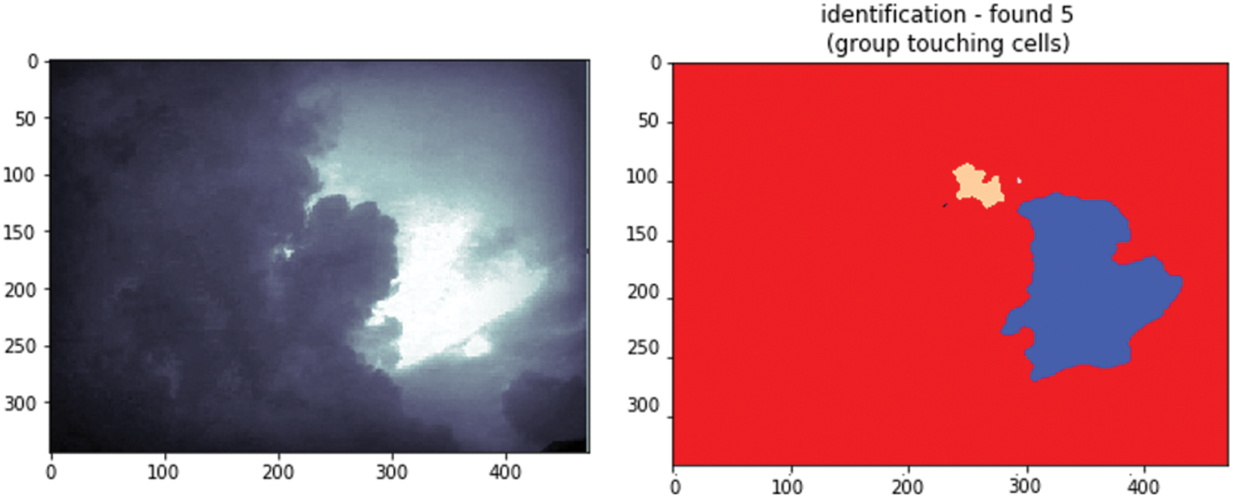
Figure 3: Key descriptive features and Difference of Gaussian (DoG)

As shown in Eq. (7); H are the significant KPs in the dataset D which consists upon the DF candidates where a are significant larger set of objects whereas β are the smaller set of objects having less probability however a qualifying ratio r=a  /β is said to be sufficient for SIFT to reach at a decision [31]. Traversing of H is to be conducted from the vectors of Dxx+Dyy where SCM Dxx  Dyy−Dxy2 are persisting with the ratio of R=Tr(H)2Det  (H) which +h is to be estimated equal in terms of DF(r+1)2r. R quantities are the minimum tigers when become equal to KPs and DFs. However KPs are the candidate keys in dataset D extracted from the training or testing images by defining the (rth+1)2rth values. At this stage the object detection uses images gradient directions by rotating to inversing at local level. Every pixel of image is smoothed by using Gaussian smooth function L  (x,  y,  σ) where mean values are filled at objects designated as L by partitioning the magnitude of every image m  (x,y)and difference of previously computed variables θ  (x,y) as shown in Eqs. (8), (9) and Fig. 4.

m(x,y)=L(x+1,y)−L(y−1,y))2)+L((x,y+1,y)−L(x,y−1))2)(8)

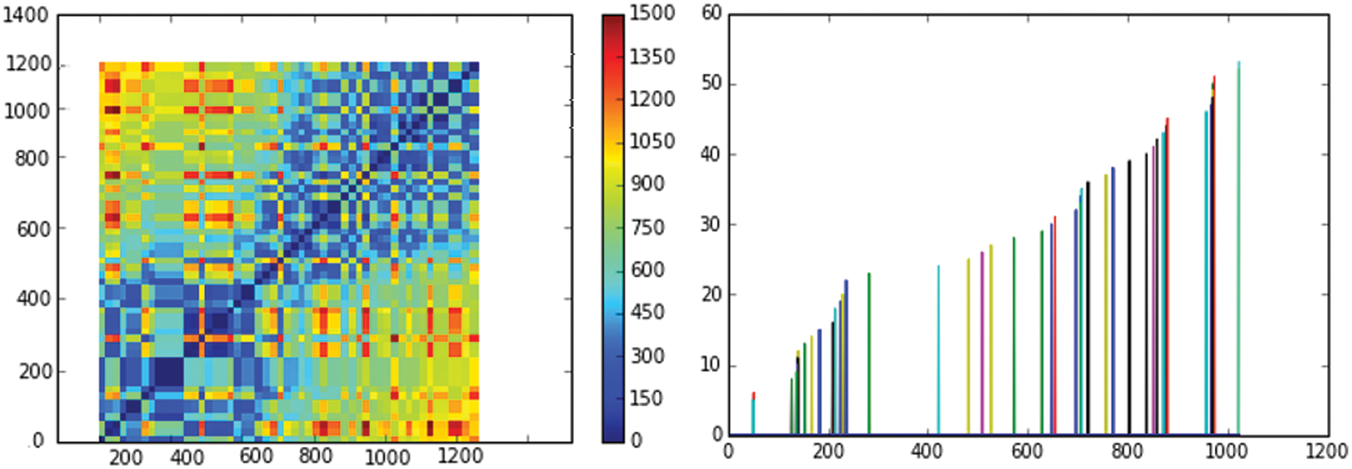
Figure 4: Finding the Feature Matching (FM) and Feature Indexing (FI) process

Neighboring pixel quantities are estimated as per above equation on the basis of gradient of pixels each bin can be computed with 3 neighboring bins KPs and DFs are matched [32–35].

θ(x,y)=atan2(L(x,y+1)−L(x,y−1),L(x1,y)−(x−1,y))(9)

d. Tensor Flow Data Conversion

Let's consider all explored scale objects in the format of invariant features as represented through SIFT operations. Considering Key points (KPs) and descriptive features (DFs) under the feature vectors of scale space structure (SSS) of the cloud objects. The transformation of all invariant objects contains sufficient content to be converted in tensor flow data for deep learning where color structure based features are recorded as per Eqs. (10) and (11).

G=(f¯x2¯fxfyf¯xf¯yfy2)(10)

G=(Rx2+Gx2+Bx2¯RxRy+GxGy+BxByRxRy+GxGy+BxBy¯Ry2+Gy2+By2)(11)

A convolutional neural network (CNN) based model was constructed by using the pixel information of cloud images after the preprocessing steps as stated above section. we converted SIFT features into the tensor flow pkl  file where tensor T data type is to be processed from various inputs layers, hidden layers, pooling and fully connected layers. The CNN gradient vectors loaded with the pixel information derived from the dataset D where all the object shapes and features were considered as gradient of (f) and gx  +  yx [36,37]. The features coordinates such as (x,y) represents the shape on the bases of z variable where each pixel intensity is considerable amount of information which can be used to train and test the CNN architecture [38].

e. Input Layer of Proposed Model

We inputted a 3 dimensional cloud data as derived from the SIFT features. The input layer of convolutional neural network is comprising over three dimensions 28 × 28 × 1 which is 784 as represented into three dimensional matrix and reshaped into single column where m training observation will input 784, m size of inputs as shown in Fig. 5.

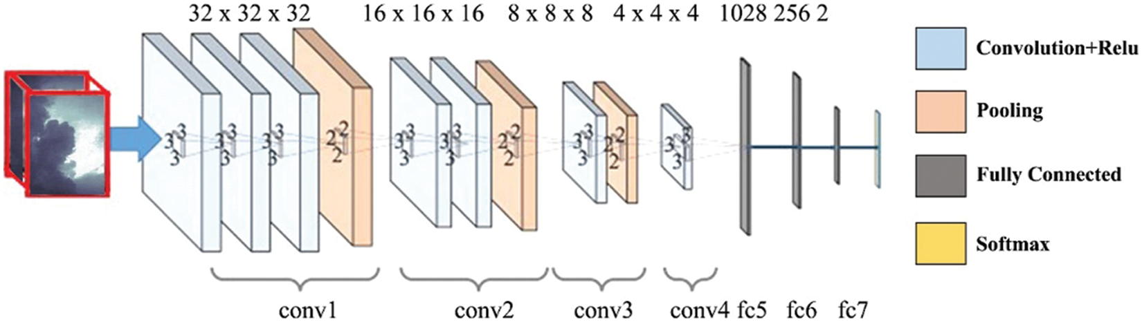
Figure 5: Convolutional neural network architecture

f. Convolutional Layer

We extracted the features of cloud images by using the Convolutional layer, since each part of 28 × 28 matrix is loaded into a feature vector where each portion of cloud image connects to the receptive field because conv layer is responsible to perform the convolutional operation, mostly the result of convolutions is formed in shape of product and receptive field which s combination of local region in connection with region, the requirement could as same size of filter. The receptive fields are being visited by using a stride and ever pixel is examined and final outputs are supplied to ReLue activation which makes all negative quantities to zero. Then the outputs are supplied to pooling layer which performs reduction in spatial volumes as supplied to pooling layer as input. The layer deals with the variables among convolutional layer and fully connected layer. Since the without using max pool or layer there are fare chances for computationally expensive results because max performs reduction in spatial volumes into the input image. 4 ×4 dimensional views could be observed with stride 2 under the surface of max pool layer. There is no parameter in pooling layer but it has two hyper parameters—Filter (F) and Stride (S). In general, if we have input dimension W1 × H1 × D1, then

W2=(W1−F)/S+1

H2=(H1−F)/S+1(12)

D2=D1

where W2, H2 and D2 are the width, height and depth of output as per Eq. (12).

g. Fully Connected and Output Layers

The variables of dot product are assigned to fully connected layer and it also hold the softmax layer where fully connected layer has to produce classification results upon the output layer. The fully connected layer not only connects all the neurons but it tackles weights and biases as well. Fully connected layer involves weights, biases, and neurons.

h. Performance

The performance of our proposed framework have been investigated by using the confusion matrix. The matrix holds the quantities in terms of true positive and true negative number of observation whereas precision measure holds the number of true positive observations and determines that how the system has understood training data. The recall measure shows that what is the capability of constructed model to identify the new instances.

Accuracy=TP+TNNX100(13)

=PrecessionTPTP+FP(14)

Recall=TPTP+FN(15)

We approximated accuracy as Eq. (13) whereas precision as per Eq. (14) and recall measure as Eq. (15).

4  Results and Discussion

This paper offers a framework for prediction of precipitation and classifies cloud objects using convolutional neural network. Cloud image data was extracted from social media applications in video format and converted into images by considering the significance of video frames. As use case we selected 100 videos for extracting the images from the frame sequences of video data. Around 2000 cloud images were selected for training and testing purposes. In data preparation layer our approach performs noise reduction by using SIFT features and convert them into tensor flow data where feature matching (FM) and feature indexing (FI) are descriptive vectors are trained to recognize the patterns of cloud images. As per Figs. 3 and 4 the method searches FM and FI from the images by estimating the nearest neighborhood set of pixels with highest probabilities under the limited computational time. The BBF algorithm keep the quantities of features in bins and feature space finds closest path distance to search the required patterns. KP with minimum KPs are search by mapping the minimal Euclidean distances from the descriptive vectors (DV). SIFT framework that creates KPs to detect the objects by convolving Gaussian filters at various scales and followed by the KPs are pointed with maximum and minim quantities of difference of Gaussian (DoG) at various scales. DoG image could be represented as D  (x,  y,  σ) where image D has x,  y location summarized as G  (x,  y,  kσ) aid ∂ is the average of ICM at every pixel as shown in Fig. 2. After acquiring the key features and pattern detection, the tensor flow features of objects were acquired to train the CNN classifier to find out deepest knowledge of cloud data. The precipitation = yes and precipitation = no class label attribute were assigned by the nature of pictures. Confusion matrix results show that precipitation = yes class classified 612 observation and misclassified 37 instances whereas precision was recorded as 94.29% and recall measure 94.73% was estimated as shown in Tabs. 1 and 2. In Class label attribute precipitation = no class classified 1611 observations and misclassified 34 observations, whereas precision was recorded as 97.93% and recall measure was estimated as 97.75%, meanwhile overall classification estimation was measured as 96.90% as shown in Tab. 3.

5  Conclusion

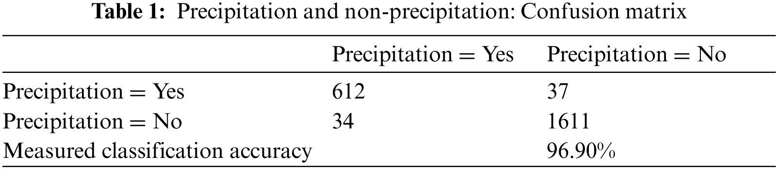
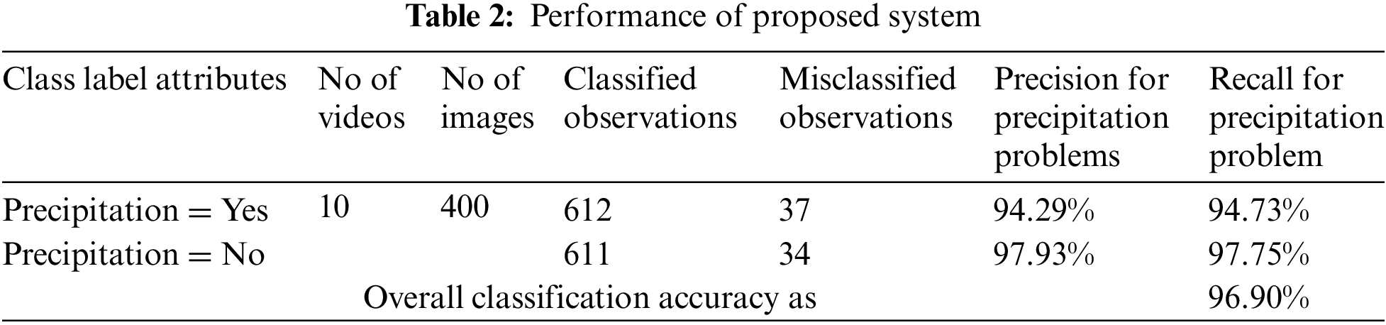
Weather prediction is an important problem for every business but particularly precipitation prediction (PP) would provide more assistance to farmers to grow crops in their fields; Deep learning techniques are frequently used to predict the weather variables (WV). We use cloud image data captured from the frames of videos pertaining the information of precipitation from social medical applications such as Facebook. As use case we selected 100 videos for extracting the images from the frame sequences of video data. Around 2000 cloud images were selected for training and testing purposes. However, dark cloud patterns (DCP) with variant grey appearance (VGA) are very hard to detect and to consider for training of machine learning algorithms. Identification clouds would provide more meticulous assistance to the common people to know about the weather conditions at their region. This research proposes a framework to classify the dark cloud patterns (DCP) for precipitation prediction (PP). The framework consists upon three steps, first step tackles noise reduction operations, feature selection and preparation of datasets. Second steps construct the decision model and third step presents the results visualization by using confusion matrix, precision, recall and accuracy measures. Confusion matrix results show that precipitation = yes class classified 612 observation and misclassified 37 instances whereas precision was recorded as 94.29% and recall measure 94.73% was estimated. In Class label attribute precipitation = no class classified 1611 observations and misclassified 34 observations, whereas precision was recorded as 97.93% and recall measure was estimated as 97.75%, meanwhile overall classification estimation was measured as 96.90%. This research contributes (1) real-world clouds datasets (2) method to prepare datasets (3) highest classification accuracy to predict PP problem measured as 96.90%.

Acknowledgement: We shall remain thankful to the Department of Computer Science, Shah Abdul Latif University for providing a nice environment to conduct the research.

Funding Statement: The authors received no specific funding for this study.

Conflicts of Interest: The authors declare that they have no conflicts of interest to report regarding the present study.

References

 1.  F. Liu, O. Yu, W. Wang, Y. Jing, L. Jian et al., “Seasonal evolution of the intraseasonal variability of China summer precipitation,” Climate Dynamics, vol. 54, no. 11, pp. 4641–4655, 2020. [Google Scholar]

 2.  Bhuiyan, M. A. Ehsan, Y. Feifei, K. B. Nishan, H. R. Saiful et al., “Machine learning-based error modeling to improve GPM IMERG precipitation product over the Brahmaputra river basin,” Advances in Hydrological Forecasting, vol. 2, no. 3, pp. 248–266, 2020. [Google Scholar]

 3.  G. Ayzel, S. Tobias and H. Maik, “RainNet v1.0: A convolutional neural network for radar-based precipitation nowcasting,” Geoscientific Model Development, vol. 13, no. 6, pp. 2631–2644, 2020. [Google Scholar]

 4.  H., Zeng-Zhen, K. Arun, J. Bhaskar and H. Boyin, “How much of monthly mean precipitation variability over global land is associated with SST anomalies?,” Climate Dynamics, vol. 54, no. 1, pp. 701–712, 2020. [Google Scholar]

 5.  Y. Liu, L. Dejuan, W. Shaohua, W. Fan, D. Wanchun et al., “A long short-term memory-based model for greenhouse climate prediction,” International Journal of Intelligent Systems, vol. 37, no. 1, pp. 135–151, 2021. [Google Scholar]

 6.  R. J. Brulle, “Networks of opposition: A structural analysis of US climate change countermovement coalitions 1989–2015,” Sociological Inquiry, vol. 91, no. 3, pp. 603–624, 2021. [Google Scholar]

 7.  S. Pandya, G. Hemant, S. Anirban, A. Muhammad, K. Ketan et al., “Pollution weather prediction system: Smart outdoor pollution monitoring and prediction for healthy breathing and living,” Sensors, vol. 20, vol. 18, pp. 5448, 2020. [Google Scholar]

 8.  A. C. Mandal and P. S. Om, “Climate change and practices of farmers’ to maintain rice yield: A case study,” International Journal of Biological Innovations, vol. 2, no. 1, pp. 42–51, 2020. [Google Scholar]

 9.  D. Ahmad and A. Muhammad, “Climate change adaptation impact on cash crop productivity and income in Punjab province of Pakistan,” Environmental Science and Pollution Research, vol. 27, pp. 30767–30777, 2020. [Google Scholar]

10. G. V. A. fzali, K. Subodh, N. Phu, H. Kuo-lin, S. Soroosh et al., “Deep neural network cloud-type classification (DeepCTC) model and its application in evaluating PERSIANN-CCS,” Remote Sensing, vol. 12, no. 2, pp. 316, 2020. [Google Scholar]

11. Z. M. Abbood and T. A. Osama, “Data analysis for cloud cover and rainfall over Baghdad city, Iraq,” Plant Archives, vol. 20, no. 1, pp. 822–826, 2020. [Google Scholar]

12. Y. Bo-Young, J. Eunsil, S. Seungsook and L. GyuWon, “Statistical characteristics of cloud occurrence and vertical structure observed by a ground-based Ka-band cloud radar in South Korea,” Remote Sensing, vol. 12, no. 14, pp. 2242, 2020. [Google Scholar]

13. N. Ayasha, “A comparison of rainfall estimation using himawari-8 satellite data in different Indonesian topographies,” International Journal of Remote Sensing and Earth Sciences (IJReSES), vol. 17, no. 2, pp. 189–200, 2021. [Google Scholar]

14. C. Zhou, X. Jinge and L. Haibo, “Multiple properties-based moving object detection algorithm,” Journal of Information Processing Systems, vol. 17, no. 1, pp. 124–135, 2021. [Google Scholar]

15. J. Wang, W. Ran and Y. Xiaqiong, “An algorithm of object detection based on regression learning for remote sensing images,” Journal of Physics: Conference Series, vol. 1903, no. 1, pp. 12039, 2021. [Google Scholar]

16. R. Raja, K. Sandeep and M. Rashid, “Color object detection based image retrieval using ROI segmentation with multi-feature method,” Wireless Personal Communications, vol. 112, no. 1, pp. 169–192, 2020. [Google Scholar]

17. M. Zhao, H. C. Chorng, X. Wenbin, X. Zhou and H. Jinyong, “Cloud shape classification system based on multi-channel cnn and improved fdm,” IEEE Access, vol. 8, pp. 44111–44124, 2020. [Google Scholar]

18. I. S. Bajwa and H. S. Irfan, “PCA based image classification of single-layered cloud types,” in Proc. of the IEEE Symp. on Emerging Technologies, Islamabad, Pakistan, vol. 1, pp. 365–369, 2005. [Google Scholar]

19. Tian Bin, S. Mukhtiar, R. Mahmood, H. Thomas et al., “A study of cloud classification with neural networks using spectral and textural features,” IEEE Transactions on Neural Networks, vol. 10, no. 1, pp. 138–151, 1999. [Google Scholar]

20. S. Dev, H. L. Yee and W. Stefan, “Categorization of cloud image patches using an improved texton-based approach,” in 2015 IEEE Int. Conf. on Image Processing (ICIP), Quebec City, QC, Canada, pp. 422–426, 2015. [Google Scholar]

21. Z. Wu, X. Xian, X. M. Min and L. Lin, “Ground-based vision cloud image classification based on extreme learning machine,” The Open Cybernetics & Systemics Journal, vol. 9, no. 1, pp. 2877–2885, 2015. [Google Scholar]

22. G. Terrén-Serrano and M. R. Manel, “Comparative analysis of methods for cloud segmentation in ground-based infrared images,” Renewable Energy, vol. 175, pp. 1025–1040, 2021. [Google Scholar]

23. A. Yu, T. Ming, L. Gang, H. Beiping, X. Zhongwei et al., “A novel robust classification method for ground-based clouds,” Atmosphere, vol. 12, no. 8, pp. 999, 2021. [Google Scholar]

24. Y. Tang, Y. Pinglv, Z. Zeming, P. Delu, C. Jianyu et al., “Improving cloud type classification of ground-based images using region covariance descriptors,” Atmospheric Measurement Techniques, vol. 14, no. 1, pp. 737–747, 2021. [Google Scholar]

25. S. Liu, D. Linlin, Z. Zhong, C. Xiaozhong and S. D. Tariq, “Ground-based remote sensing cloud classification via context graph attention network,” IEEE Transactions on Geoscience and Remote Sensing, vol. 60, pp. 1–11, 2021. [Google Scholar]

26. C. Papageorgiou and T. Poggio, “A trainable system for object detection,” International Journal of Computer Vision, vol. 38, no. 1, pp. 15–33, 2000. [Google Scholar]

27. Y. Pang, X. Zhao, L. Zhang and H. Lu, “Multi-scale interactive network for salient object detection, ” in Proc. of the IEEE/CVF Conf. on Computer Vision and Pattern Recognition, Seattle, WA, USA, pp. 9413–9422, 2020. [Google Scholar]

28. W. Wang, B. Xiang, L. Wenyu and J. L. Longin Jan, “Feature context for image classification and object detection,” in CVPR 2011, Colorado Springs, IEEE, pp. 961–968, 2011. [Google Scholar]

29. S. Nilufar, R. Nilanjan and Z. Hong, “Object detection with DoG scale-space: A multiple kernel learning approach,” IEEE Transactions on Image Processing, vol. 21, no. 8, pp. 3744–3756, 2012. [Google Scholar]

30. W. Fang, D. Yewen, Z. Feihong and S. Victor, “DOG: A new background removal for object recognition from images,” Neurocomputing, vol. 361, pp. 85–91, 2019. [Google Scholar]

31. S. Zhang, T. Qi, H. Gang, H. Qingming and L. Shipeng, “Descriptive visual words and visual phrases for image applications,” in Proc. of the 17th ACM Int. Conf. on Multimedia, 2000, Lisboa, Portugal, pp. 75–84, 2000. [Google Scholar]

32. C. Wang and H. Kaiqi, “How to use bag-of-words model better for image classification,” Image and Vision Computing, vol. 38, pp. 65–74, 2015. [Google Scholar]

33. P. M. Choksi, S. D. Laxmi and K. M. Yogesh, “Object detection using deep learning for visually impaired people in indoor environment,” in Soft Computing and Signal Processing, vol. 2021, Singapore: Springer, pp. 617–625, 2021. [Google Scholar]

34. J. G. Shanahan and D. Liang, “Introduction to computer vision and real time deep learning-based object detection,” in Proc. of the 26th ACM SIGKDD Int. Conf. on Knowledge Discovery & Data Mining, 2020, Virtual Event, CA, USA, pp. 3523–3524, 2020. [Google Scholar]

35. M. Kartal and D. Osman, “Ship detection from optical satellite images with deep learning,” in 2019 9th Int. Conf. on Recent Advances in Space Technologies (RAST), Istanbul, Turkey, vol. 2019, pp. 479–484, 2019. [Google Scholar]

36. A. Dasgupta and S. Sonam, “A fully convolutional neural network based structured prediction approach towards the retinal vessel segmentation,” in 2017 IEEE 14th Int. Symp. on Biomedical Imaging (ISBI 2017), Melbourne, VIC, Australia, pp. 248–251, 2017. [Google Scholar]

37. Y. D. Zhang, P. Chichun, S. Junding and T. Chaosheng, “Multiple sclerosis identification by convolutional neural network with dropout and parametric ReLU,” Journal of Computational Science, vol. 28, pp. 1–10, 2018. [Google Scholar]

38. S. K. Lee, L. Hwajin, B. Jiseon, A. Kanghyun, Y. Youngsam et al., “Prediction of tire pattern noise in early design stage based on convolutional neural network,” Applied Acoustics 2021, vol. 172, pp. 107617, 2021. [Google Scholar]

This work is licensed under a Creative Commons Attribution 4.0 International License, which permits unrestricted use, distribution, and reproduction in any medium, provided the original work is properly cited.